Oxygen concentration in the South Adriatic Sea: the gliders measurements - OGS

ISTITUTO NAZIONALE di Oceanografia e di Geofisica Sperimentale Trieste

 Oxygen concentration in the South Adriatic Sea:
 the gliders measurements.

 Gerin R., Martellucci R., Mauri E., Kokkini Z., Medeot N., Nair R., Zuppelli P.,
 Comici C. and Pachou A.

Borgo Grotta Gigante, 09/06/2020 Rel. 2020/36 Sez. OCE 11 MAOS Page 1 of 31

ISTITUTO NAZIONALE di Oceanografia e di Geofisica Sperimentale Trieste

 SOMMARIO:

 Introduction 3
 Preliminary comparison of Glider data with Oceanographic campaigns in South Adriatic Sea 3
 Methods for measuring dissolved oxygen concentration 4
 Winkler 4
 Optical sensors 4
 Yearly oxygen data comparison 5
 Evaluation of the temperature as measured by the oxygen sensor 10
 Oxygen computation from phase data 11
 Optode configuration coefficients in gliders 12
 Salinity compensation of data 13
 Depth compensation of data 13
 Compensated oxygen concentration 14
 Lab tests 16
 In-situ “calibration” of the glider oxygen data 17
 Glider and float oxygen data comparison 21
 Best fit line using least square minimization of the glider oxygen data 25
 Drift of the oxygen sensor with time (Slocum 403 case) 27
 Oxygen drift due to foil: Aanderaa factory indications 28
 Possible correction for the oxygen glider data without a reference 28
 Final results 29
 Acknowledges 29
 References 30
 Internet References 31

Borgo Grotta Gigante, 09/06/2020 Rel. 2020/36 Sez. OCE 11 MAOS Page 2 of 31

ISTITUTO NAZIONALE di Oceanografia e di Geofisica Sperimentale Trieste

Introduction

In this report we explored the oxygen data recorded by 4 different gliders (2 Slocum SN 402 and
403 and 2 SeaGlider SN SG554 and SG661) in the South Adriatic Pit. A first comparison with
other available oxygen data (from floats, CTDs profiles or Winkler samples) in the area evidenced
a large difference of the glider oxygen values with respect to the other data. Moreover, a detailed
analysis demonstrated that the SeaGlider data seem to overestimate the floats/CTDs/Winkler
data, while the Slocum data underestimate them.

The data analysis pointed out two main issues:
 ● the need of compensate the glider oxygen data for the depth and salinity;
 ● the need of in-situ correct/calibrate the glider oxygen data.

These issues were investigated throughout the report and a final homogeneous dataset with
validated, corrected and compensated oxygen values were obtained for all the glider missions.

Preliminary comparison of Glider data with Oceanographic
campaigns in South Adriatic Sea

The Adriatic Sea is an elongated basin, with its major axis in the northwest–southeast direction,
located in the central Mediterranean Sea, between the Italian and the Balkan peninsula. Countries
with coasts on the Adriatic Sea are Albania, Bosnia and Herzegovina, Croatia, Greece, Italy,
Montenegro and Slovenia. Being located at mid latitudes, the Adriatic Sea is characterized on
one hand by a strong seasonal variability and on the other hand by synoptic weather variations,
which are in turn modulated by the seasonal signal (Gacic et al., 2001). The southern part is
characterized by a large depression that reaches more than 1200 m depth. The water exchange
with the Mediterranean Sea takes place through the Otranto Channel, whose sill is about 800 m
deep.

Generally, the whole Adriatic Sea is a well-oxygenated basin. During spring and summer a
subsurface maximum is formed in the euphotic zone, between approximately 10 and 50 m, due
to biological activity that results in a net production of oxygen near the pycnocline after the density
stratification of the water column has become established. In autumn and winter ventilation at the
surface and water column mixing create a more homogeneous oxygen distribution. The average
basin value of dissolved oxygen is approximately 5.5 ml l−1 (Artegiani et al., 1997, Vilibic et al.
2002).

Borgo Grotta Gigante, 09/06/2020 Rel. 2020/36 Sez. OCE 11 MAOS Page 3 of 31

ISTITUTO NAZIONALE di Oceanografia e di Geofisica Sperimentale Trieste

Methods for measuring dissolved oxygen concentration
Oxygen measurements can be obtained directly with an analytic analysis and indirectly by means
of electrochemical measurements. The Winkler titration is the most accurate and widely adopted
method to estimate the oxygen concentration in the water from punctual samples. The oxygen
concentration that is obtained by the Winkler method allows to calibrate oxygen measurement
obtained with oxygen probes that sample continuously all along the water column. There are
different kind of sensors which derive the oxygen concentration using different physical
principles/characteristics as the electrochemistry (Clark electrode or polarographic system) or the
optic.

Winkler
The chemical determination of oxygen concentrations in seawater is based on the method
proposed by Winkler (1888) and modified by Strickland and Parsons (1968).
The Winkler analysis of dissolved oxygen has different steps. A seawater sample, that hasn't
been exposed to additional oxygen source, is "fixed" by adding a series of reagents that form an
acid compound that is then titrated with a neutralizing compound. The amount of neutralizing
agent required to neutralize the acid with titration indicates the amount of oxygen present in the
original sample. The procedure is particularly delicate and susceptible to human error.

Optical sensors
Optical sensors mounted on CTD or autonomous profiling instruments provide direct in-situ
measurements of oxygen. Among all the different kind of sensors on the market, we would
consider the Seabird SBE 43 usually mounted on CTD and Floats and the Aanderaa Oxygen
Optode usually mounted on Gliders and Floats.
The SBE 43 is a high-accuracy oxygen sensor which determines the dissolved oxygen
concentration by counting the number of oxygen molecules per second (flux) that diffuse through
a membrane from the ocean environment to an electrode. At the electrode, the oxygen gas
molecules are converted to hydroxyl ions (OH-) in a series of reaction steps. The reaction is then
completed by the electrode which supplies four electrons per molecule. The sensor counts oxygen
molecules by measuring the electrons per second delivered to the reaction. At another electrode,
silver chloride is formed and silver ions (Ag+) are dissolved into solution. As a result, the chemistry
of the electrolyte changes continuously as oxygen is measured, which leads to a slow but
continuous loss of sensitivity that produces a continual, predictable drift in the sensor calibration
over time.
The SBE 43 is designed to be used in a CTD’s pumped flow path, providing optimal correlation
with CTD measurements (http://www.seabird.com/sbe43-dissolved-oxygen-sensor &
http://www.seabird.com/document/an64-sbe-43-dissolved-oxygen-sensor-background-
information-deployment-recommendations).

The Aanderaa oxygen Optodes are based on the ability of selected substances to act as dynamic
fluorescence quenchers. The luminous indicator is a special platinum – porphyrin complex set
inside a gas permeable foil that is exposed to the surrounding water. The foil is excited by
modulated blue light, and the Optode measures the phase shift of a returned red light The sensor

Borgo Grotta Gigante, 09/06/2020 Rel. 2020/36 Sez. OCE 11 MAOS Page 4 of 31

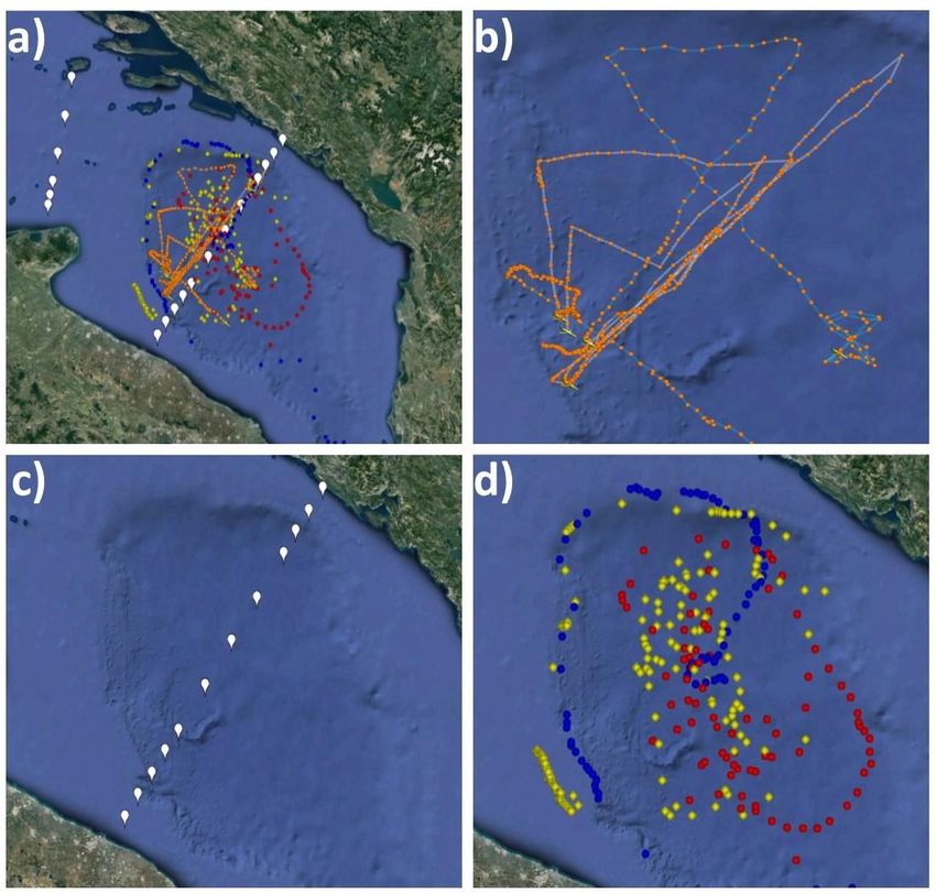
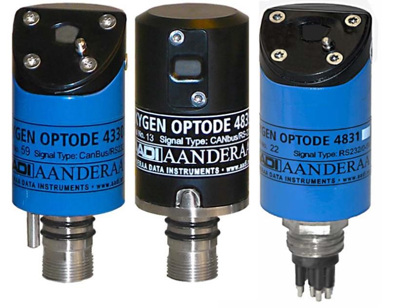
ISTITUTO NAZIONALE di Oceanografia e di Geofisica Sperimentale Trieste

has an incorporated temperature thermistor that enables linearization and temperature
compensation of the phase measurements in order to provide the absolute O2 concentration.

The Seaglider and the Slocum gliders considered in this report are equipped with the Oxygen
Optode 4330/4330F and the Oxygen Optode 4831/4831F, respectively
(http://www.aanderaa.com/media/pdfs/oxygen-optode-4330-4330f.pdf &
http://www.xylemanalytics.co.uk/media/pdfs/4330-4330f-oxygen-optode_dec12.pdf,
http://www.xylemanalytics.co.uk/media/pdfs/aanderaa-oxygen-optode-4831-4831f.pdf).

Yearly oxygen data comparison
The oxygen concentration obtained from the Winkler method and from different optical sensors
mounted on several platforms such as Argo floats, Gliders and CTDs were compared using all
the available data collected in the South Adriatic Sea between 2013 and 2017 (Figs 1 and 2).

Fig. 1: Geographical position of the different measuring platform (a), glider surfacing during different glider
 mission (b), CTD/Winkler stations during oceanographic cruises (c) and float profiles (d) in the South
 Adriatic Sea (6901865 blue circles; 6903178 yellow circles and 6903197 red circles).

Borgo Grotta Gigante, 09/06/2020 Rel. 2020/36 Sez. OCE 11 MAOS Page 5 of 31

ISTITUTO NAZIONALE di Oceanografia e di Geofisica Sperimentale Trieste

 Fig. 2: Time intervals of the available oxygen data; y axis reports the
 platform/cruise/mission name.

Data were grouped by year, without considering the spatial variability, obtaining five distinct cases
(Table 1).

 Table 1: Available oxygen data divided by platform and year. The black slots indicate the platforms
 considered in the 5 selected cases.

Borgo Grotta Gigante, 09/06/2020 Rel. 2020/36 Sez. OCE 11 MAOS Page 6 of 31

ISTITUTO NAZIONALE di Oceanografia e di Geofisica Sperimentale Trieste

Before the comparison, the oxygen data were all converted to same units (ml/l). In particular, the
float oxygen data are usually provided in μmole/Kg and were converted to ml/l following Bittig et
al. (2016):

 [μmole/kg] =[ml/l] * 44660/(sigma_theta(P=0,Theta,S)+1000)

where:

 ● sigma_theta is the density of a water parcel if it was raised adiabatically to the sea surface,
 keeping the salinity stable.
 ● P= Pressure = 0
 ● Theta is the potential temperature
 ● S= Salinity

The oxygen data comparison of the 5 cases are presented in Figs from 3 to 7. The data collected
with gliders, floats, CTD and the data obtained from Winkler samples are plotted in green, purple,
red and blue, respectively.

 Fig. 3: Profiles of oxygen concentration obtained by the different platforms for case 1 in 2013 (Winkler, CTD and
 Glider).

Borgo Grotta Gigante, 09/06/2020 Rel. 2020/36 Sez. OCE 11 MAOS Page 7 of 31

ISTITUTO NAZIONALE di Oceanografia e di Geofisica Sperimentale Trieste

 Fig. 4: Same as Fig. 3 for case 2 in 2014 (Winkler, CTD, Glider and Float).

 Fig. 5: Same as Fig. 3 for case 3 in 2015 (Winkler, CTD, Glider and Float).

Borgo Grotta Gigante, 09/06/2020 Rel. 2020/36 Sez. OCE 11 MAOS Page 8 of 31

ISTITUTO NAZIONALE di Oceanografia e di Geofisica Sperimentale Trieste

 Fig. 6: Same as Fig. 3 for case 4 in 2016 (Winkler, CTD, Glider and Float).

 Fig. 7: Same as Fig. 3 for case 5 in 2017 (Glider and Float).

Borgo Grotta Gigante, 09/06/2020 Rel. 2020/36 Sez. OCE 11 MAOS Page 9 of 31

ISTITUTO NAZIONALE di Oceanografia e di Geofisica Sperimentale Trieste

The comparison of all oxygen measurements shows the same oxygen shape along the water
column. The maximum concentration is measured in the surface layer and a second oxygen
maximum is observed between 200 and 400 m depth. At deeper layers, the oxygen remained
almost stable. The oxygen concentration varied from 4.4 to 5.8 ml/l for the floats, from 4.5 to 5.8
ml/l for the CTDs and the Winkler samples and between 3.8 and 6.2 ml/l for the gliders.
The oxygen profiles obtained from the floats, CTDs and Winkler data seems to be in a better
agreement than the one measured with the glider. In 2013 and 2014, the oxygen concentrations
from gliders are overestimated, while in 2015, 2016 and 2017 concentrations are underestimated.
In the first case, the measurements were performed by the SeaGlider SG554, while in the second
case by the Slocum glider 403, both equipped with Aanderaa Optode oxygen sensor. The
possible reason for the observed difference may be due to hardware and/or software problem.
No evident hardware issues were detected, therefore we investigate the possible software
problems considering a wrong and/or different sensors calibration or possible differences in the
computing of the oxygen concentrations from the raw (phase) data.

Evaluation of the temperature as measured by the oxygen sensor

The Oxygen Aanderaa Optode sensor use the temperature recorded by itself for computation of
the oxygen concentration.
The old Optode model (3835) recorded inaccurate temperature data due to the stagnancy of the
water in the glider tail cone where the sensor was positioned (the temperature probe of this
oxygen sensor is located on the back of the sensor, pointing towards the inside of the glider tail
cone). For this specific model the temperature recorded by the glider CTD must be used to
compute the correct oxygen concentration.
The temperature measured by the Optode sensors mounted on our gliders instead is coherent
with the CTD values as demonstrated in Fig.8 and, therefore, the observed differences of the
glider oxygen data with respect to the other oxygen data are not due to an inaccurate temperature
in the computation.

 Fig.8 Temperature profiles recorded by the CTD (blue) and by the Oxygen
 sensor (red) mounted on the Slocum 403 and the SeaGlider SG554 (left and right, respectively)

Borgo Grotta Gigante, 09/06/2020 Rel. 2020/36 Sez. OCE 11 MAOS Page 10 of 31

ISTITUTO NAZIONALE di Oceanografia e di Geofisica Sperimentale Trieste

 Oxygen computation from phase data

 The Aanderaa Optode oxygen sensor is influenced by temperature, salinity and pressure that
 modify the hardware response of the sensor. As a consequence, a compensation is needed.

 A check of the computational steps was performed following the Aanderaa TD269 Oxygen optode
 operating manual (2017).

 From the raw data the difference between the phase obtained with blue (C1Phase) and red light
 (C2Phase) excitation is calculated as:

 TPhase = A( t ) + ( C1Phase − C2Phase ) ⋅ B( t )

 The A(t) and B(t) are temperature-dependent 3rd order polynomials that give a temperature
 compensation of the measured phase. Usually, as in our case, this compensation is not performed
 and A(t)=0, B(t)=1.

 Thus the CalPhase is computed as:

CalPhase = PhaseCoef0 + PhaseCoef1 ⋅ TPhase + PhaseCoef2 ⋅ TPhase2 + PhaseCoef3 ⋅ TPhase3

 Based on the CalPhase and the temperature, the partial pressure of O2 is calculated using a two
 dimensional polynomial:

 ∆ p = C0 ⋅ t m0 ⋅ ph n0 + C1 ⋅ t m1 ⋅ ph n1 + C2 ⋅ t m2 ⋅ ph n2 + ... + C27 ⋅ t m27 ⋅ ph n27

 where the polynomial coefficients C0 to C13 are recorded in the property FoilCoefA and C14 to
 C27 are stored in FoilCoefB. The temperature exponents are stored as FoilPolyDegT and the
 phase exponents are recorded as FoilPolyDegO.

 The air saturation is then calculated as:
 ∆ ⋅ 100
 AirSaturation ( % ) =( − ( ) ⋅ )

 with:

 NomAirPress = 1013.25 hPa,
 NomAirMix is the nominal O2 content in air, by default 0.20946 and
 Pvapour (t) = e (52.57 - (6690.9 / (t+ 273.15)) - 4.681 * ln (t+ 273.15)

 If the property Enable HumidityComp is set to ‘No’ the Pvapour (t) will be set to zero.

 The oxygen concentration is finally computed as:

 ∗ ⋅ 44.614 ⋅ 
 O2 Concentration ( μM ) = ( )
 100

 where C* is the oxygen solubility (cm3/dm3) calculated from the Garcia and Gordon equation of
 1992:

 Borgo Grotta Gigante, 09/06/2020 Rel. 2020/36 Sez. OCE 11 MAOS Page 11 of 31

ISTITUTO NAZIONALE di Oceanografia e di Geofisica Sperimentale Trieste

ln (C*) =A0 + A1 TS + A2 TS 2 + A3 TS 3 + A4 TS 4 + A5 TS 5 + S (B0 + B1 TS + B2 TS 2 + B3 TS 3) + C0 S 2

 where:
 298.15 − 
 TS = scaled temperature = ln ( 273.15 + )

 t = Temperature, °C
 S = Salinity, configurable property, default set to zero

 A0 = 2.00856 B0 = -6.24097e-3
 A1 = 3.22400 B1 = -6.93498e-3
 A2 = 3.99063 B2 = -6.90358e-3
 A3 = 4.80299 B3 = -4.29155e-3
 A4 = 9.78188e-1 C0 = -3.11680e-7
 A5 = 1.71069

 A possibility for linear correction of the O2 Concentration is also introduced (and used by the
 Slocum gliders):

 O2 Concentration [uM] = ConcCoefb + ConcCoefa [O2]′

 For our Slocum gliders only the ConCoefs (determined by the factory) are:

 ConcCoefa = 6.200611e-1;
 ConcCoefb = 1.018849;

 Optode configuration coefficients in gliders

 The Optode configuration coefficients can be retrieved from the Slocum glider by sending to the
 glider the u4stalk 4 9600 34 command (syntax from the Aanderaa TD269 Oxygen optode
 operating manual (2017)) and then:

 ● Stop (enter)
 ● Get All (enter)

 This will NOT work using glider terminal, the operator should use minicom or teraterm configured
 to send either Line Feed (Ascii Code 10) or Line Feed + Carriage Return (Ascii Code 10 + Ascii
 Code 13).
 After these commands, the Aanderaa Optode coefficients are displayed.

 In the case of the SeaGlider, the Aanderaa Optode configuration coefficients can be retrieved
 from the “show configuration” option of the sensor interactive menu.

 From the obtained outputs, the fundamental difference between the Optode configuration
 coefficients of the Slocum and of the SeaGlider is that the salinity reference is set to 35 for the
 Slocum glider and to 0 for the SeaGlider.

 Borgo Grotta Gigante, 09/06/2020 Rel. 2020/36 Sez. OCE 11 MAOS Page 12 of 31

ISTITUTO NAZIONALE di Oceanografia e di Geofisica Sperimentale Trieste

Salinity compensation of data

The O2 concentration is the partial pressure of dissolved oxygen in the water. Since the foil is only
permeable to gas and not to water, the Optode cannot sense the effect of salt dissolved in the
water. Hence the Optode works as if it is immersed in fresh water. In the case of the in-situ salinity
variation less than ± 1 ppt, the O2 concentration can be compensated in real-time inside the
sensor by setting the internal property ‘Salinity’ (i.e. the salinity reference) to the average
measured salinity. If the salinity varies significantly it is mandatory to perform a salinity
compensation afterward.

The compensated O2 concentration (in μM) is calculated from the following equation:

 2 3 2 − 2 )
 02 = [ 2 ] ( 0 + 1 + 2 + 3 )+ 0 ( 0

where:

S = measured salinity in psu
 298.15 − 
TS = scaled temperature = ln ( 273.15 + )
t = temperature, °C
B 0 = -6.24097e-3
C 0 = -3.11680e-7
B 1 = -6.93498e-3
B 2 = -6.90358e-3
B 3 = -4.29155e-3
S0 = salinity reference.

NOTE: Salinity compensation is not performed within the Optode, neither by the glider software.

Depth compensation of data

The Optode sensing foil response decreases with water pressure (3.2% lower response at 1000
m depth; more details in Uchida et al., 2008,). This effect is the same for all AADI oxygen Optodes
and is totally and instantly reversible and easy to compensate for.
The depth compensated O2 concentration, O2c, is calculated from the following equation:

 0.032 
 2 = 2 (1 + )
 1000
where:
d is depth in meters or pressure in dbar.

Borgo Grotta Gigante, 09/06/2020 Rel. 2020/36 Sez. OCE 11 MAOS Page 13 of 31

ISTITUTO NAZIONALE di Oceanografia e di Geofisica Sperimentale Trieste

O2 is the measured Oxygen concentration in either μM or % and the unit of the compensated
concentration, O2c, depends on the unit of the O2 input.

NOTE: Depth compensation is not performed within the Optode, neither by the glider software.

Compensated oxygen concentration

The uncompensated oxygen concentrations recorded by the Optode, with the configuration
coefficients set by the manufacturer, were corrected using the pressure (depth) and salinity
measured by the glider CTD to obtain the compensated values of the oxygen. The compensation
led to a decrease of the oxygen values of about 1 ml/l and 0.1 ml/l in the SeaGlider and the
Slocum, respectively.

 Fig.9 Compensated oxygen data of the SeaGlider (Convex14 mission) and of the Slocum (PreConvex16 mission)
 (left and right, respectively). Original data are depicted in green and compensated values in cyan.

After the compensation, glider oxygen concentrations show similar values, especially in the
deepest layers (Fig.10).

Borgo Grotta Gigante, 09/06/2020 Rel. 2020/36 Sez. OCE 11 MAOS Page 14 of 31

ISTITUTO NAZIONALE di Oceanografia e di Geofisica Sperimentale Trieste

 Fig.10 Compensated oxygen during all the glider mission between 2013 and 2017.

The contribution of the salinity to the oxygen compensation has a larger weight (Fig. 11) with
respect to the contribution of the depth (or pressure; Fig. 12).

 Fig.11 Multiplicative salinity and depth factors (left and right, respectively) for dive 11 of the Convex14
 glider mission.

Borgo Grotta Gigante, 09/06/2020 Rel. 2020/36 Sez. OCE 11 MAOS Page 15 of 31

ISTITUTO NAZIONALE di Oceanografia e di Geofisica Sperimentale Trieste

Fig.12 Multiplicative salinity and depth factors (left and right, respectively) for dive 30 of the PreConvex16
 glider mission.

The compensation procedure is very important, contributing largely in the correction of the data,
but a difference with respect to the Winkler/CTD/float values still remain (underestimation of about
0.5-0.8 ml/l; compare the blu, red and magenta lines of Figs from 3 to 7 with the compensated
values of Fig. 10).

Lab tests

To further investigate the gaps between the glider oxygen data and the data from
Winkler/CTD/float, some lab tests were run at the OGS wet laboratory to compare the
measurement of the gliders with a reference sensors and Winkler samples.

In October 2017 the Slocum gliders 402 and 403 were immersed in a salty water tank along with
a reference sensor (Aanderaa 4330F) and two 4531A sensors (brand new).
The reference sensor recorded values around 248 umol/l (5.55 ml/l) with salinity reference of 0
(corresponding to 202 umol/l (4.52 ml/l) with salinity reference 35; the brand new sensors
recorded almost identical values). The 4831 sensors mounted on the two Slocum gliders instead
underestimated the oxygen with mean readings of 185 (4.14 ml/l) and 192 umol/l (4.3 ml/l) for the
glider unit 402 and unit 403, respectively (with salinity reference of 35). The underestimation is
therefore 17 and 10 umol/l (corresponding to 0.38 and 0.22 ml/l).

In September 2018 the Aanderaa oxygen sensor on the SeaGlider SG554 was compared with
the reference sensor 4330F. The readings of the glider Aanderaa ranges between 249 (5.57 ml/l)
and 253 umol/l (5.66 ml/l), with a mean value of 251 (5.62 ml/l), while the measurements of the
reference sensor were between 239 and 241 umol/l (5.35 and 5.4 ml/l) (Table 2; these last values
were confirmed by Winkler samples). Since both the instruments were set to a salinity reference

Borgo Grotta Gigante, 09/06/2020 Rel. 2020/36 Sez. OCE 11 MAOS Page 16 of 31

ISTITUTO NAZIONALE di Oceanografia e di Geofisica Sperimentale Trieste

of 0, it results that the Aanderaa mounted on the SeaGlider overestimates the oxygen of about
11 umol/l (0.25 ml/l).

 Table 2: Measurements performed with the Aanderaa 4330F
 reference sensor (s/n 1474) during the second test.

The tests demonstrated that the oxygen values measured with the Slocum gliders is
underestimated for about 0.2-0.4 ml/l with respect to the value obtained by the reference
instrument, while the SeaGlider measurements seems to overestimate it by about 0.2 ml/l.

Unfortunately, it was not possible to run the single point “calibration” in the under-control tank in
the same time for the two kind of gliders (about one year of gap), moreover, the gliders were
submerged in the tank without wetting the foil for 48 hours prior to test the sensors (as indicated
in the Aanderaa TD269 Oxygen optode operating manual, 2017) and therefore the tests do not
provide good and consistent results that allow for a sensor correction and a different approach
was taken.

In-situ “calibration” of the glider oxygen data

The oxygen dataset, was extended including the years 2018-2020 (not available at the beginning
of the writing of this report; Fig.13). The Preconvex19 mission was performed with the SeaGlider
661 which is equipped with an unpumped CTD; these data were corrected for the thermal lag
following (Garau et al., 2011). Data were compensated for salinity and depth and then compared
with the oxygen dataset collected and validated by dr. Garić and dr. Batistić at P-1200 L-term
station in the South Adriatic Pit (SAP; Fig. 14).

Borgo Grotta Gigante, 09/06/2020 Rel. 2020/36 Sez. OCE 11 MAOS Page 17 of 31

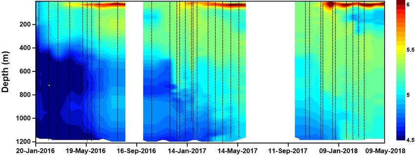
ISTITUTO NAZIONALE di Oceanografia e di Geofisica Sperimentale Trieste

 Fig. 13: Timing of the Winkler samples, profiling floats and glider missions in the South Adriatic Sea.

 Table 3: Deploy and recovery/last dates and number of days at sea of the platform/mission/cruise
 performed in the south Adriatic Sea and depicted in Fig. 13.

Glider data were also compared with the dissolved oxygen distribution recorded at the P-1200 L-
term station in the SAP (Fig. 14). During the late winter, the average concentrations is about 5.2
ml/l; the surface layer oxygen presents values of 5.5 ml/l while in the bottom layer oxygen the
dissolved oxygen decreases to about 5 ml/l. This trend was also observed in previous studies
conducted in the SAP (Artegiani et al, 1997; Zavatarelli et al., 1998; Manca et al., 2004 and Šantić
et al., 2019). The mean oxygen values measured by the glider during the same period (Fig. 15a),

Borgo Grotta Gigante, 09/06/2020 Rel. 2020/36 Sez. OCE 11 MAOS Page 18 of 31

ISTITUTO NAZIONALE di Oceanografia e di Geofisica Sperimentale Trieste

vary between 4.5 ml/l at the surface and 4 m/l at the bottom. The difference between the highest
and the lowest values along the water column measured by the glider or at the station is coherent
and is about 0.5 ml/l, while the gap between the two datasets is about 1 ml/l (the glider
underestimate).

Fig. 14: Dissolved oxygen time series recorded at P-1200 L-term station (left panel; courtesy of dr. Garić
 and dr. Batistić) and the geographic position of the station in the SAP (right panel).

Borgo Grotta Gigante, 09/06/2020 Rel. 2020/36 Sez. OCE 11 MAOS Page 19 of 31

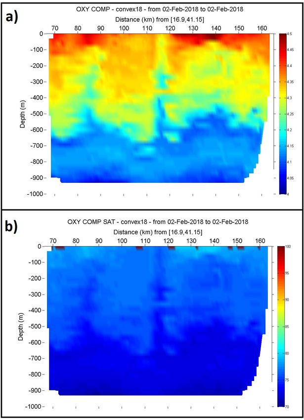
ISTITUTO NAZIONALE di Oceanografia e di Geofisica Sperimentale Trieste

 Fig. 15: Dissolved oxygen along the Bari -Dubrovnik transect in ml/l (a) and oxygen saturation (b)
 computed from the glider compensated oxygen data collected during the Convex18 glider mission.

The oxygen saturation of the glider data was evaluated (Fig. 15b) and a saturation of 85% was
observed at the surface. This value is lower than the one observed by different authors (Zavatarelli

Borgo Grotta Gigante, 09/06/2020 Rel. 2020/36 Sez. OCE 11 MAOS Page 20 of 31

ISTITUTO NAZIONALE di Oceanografia e di Geofisica Sperimentale Trieste

et al., 1998; Manca et al., 2004), therefore, also the qualitative comparison of the oxygen
saturation values of different sources confirms the underestimation of the oxygen glider data.

All the performed comparisons and analysis suggested that the oxygen values recorded by the
gliders need a careful study to be “calibrated”.

The basic idea is to use all the good available in-situ oxygen observations which are very close
in time and space to the glider data to obtain robust calibration coefficients.

For the sake of clarity, we included the term calibration in double quote. Indeed, although the
procedure can provide calibration coefficients for the oxygen sensor, we will not change the
coefficients inside the instrument and therefore we will apply a correction rather than a calibration.

Glider and float oxygen data comparison

Among all the available data (Fig. 13 and Table 3), we considered the glider missions and only
the validated Winkler samples and/or the quality-controlled oxygen float data which were
previously Winkler-calibrated in the South Adriatic Sea (Gerin et al., 2020 and Gerin and
Martellucci, 2020). The strategy of “calibrating” the glider oxygen data with Winkler-calibrated data
from other instruments is not new and was already used with good results by Quest et al. (2015).
In particular, we selected the oxygen data within varying time and space thresholds from the glider
measurements (1 day and 50 km; 2 days and 35 Km; 3 days and 20 Km; Table 4). The profiles
collected in particular geographical areas of the SAP (i.e. the slope) characterized by very strong
variability were excluded. Unfortunately, the chosen thresholds discard all the Winkler samples
and only the Winkler-calibrated oxygen float data were considered. Additionally, for some glider
missions it was not possible to find useful oxygen data to compared with (PreConvex18 performed
by Slocum glider 402, Convex17 and Convex18 by Slocum glider 403; Table 3).

Table 4: Float ID, cycle number, date, time and position and glider ID, date, time and position used in the
comparison. Time and distance gaps between the selected profiles.

Borgo Grotta Gigante, 09/06/2020 Rel. 2020/36 Sez. OCE 11 MAOS Page 21 of 31

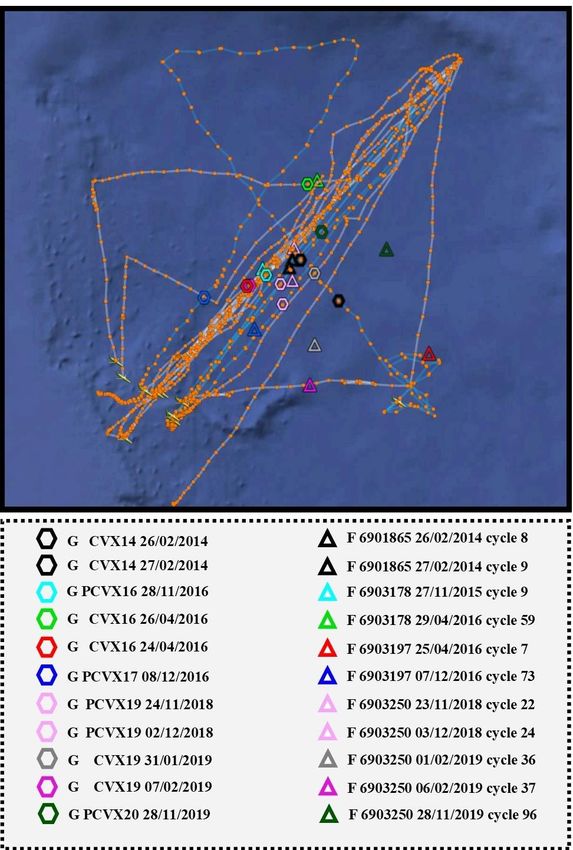
ISTITUTO NAZIONALE di Oceanografia e di Geofisica Sperimentale Trieste

Figures 16 and 17 show the location of the glider surfacings and the float profiles used in the
comparison.

 Fig. 16: Location of the glider surfacing and the float profile used in the comparison of all the cases
 selected in Table 4. Diamonds and triangles represent the glider surfacings and the float profiles,
 respectively. The symbols are color-coded with respect to time. The legend reports at the side of
diamonds the glider mission names (shortened: PCVX16 stays for Preconvex16) and the time, at the side
 of triangles the float WMO number, the time and the float cycle number.

Borgo Grotta Gigante, 09/06/2020 Rel. 2020/36 Sez. OCE 11 MAOS Page 22 of 31

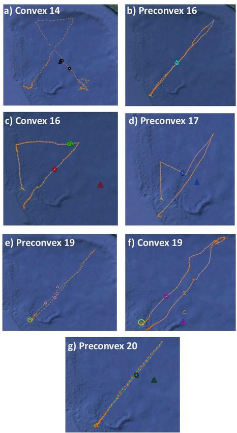
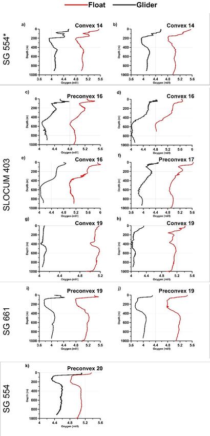
ISTITUTO NAZIONALE di Oceanografia e di Geofisica Sperimentale Trieste

 Fig. 17: Same as Fig. 16 but separated by missions: Convex14 (a); Preconvex16 (b); Convex 16 (c);
 Preconvex17 (d); Preconvex19 (e); Convex 19 (f); Preconvex20 (g).

A qualitative comparison of the glider compensated oxygen data with the selected in-situ
reference float profiles (Winkler-calibrated data; Fig. 18) evidenced a good agreement of the
profile shapes. The gaps between the glider-float profiles is not constant and it varies between
0.5 and 1.1 ml/l.

Borgo Grotta Gigante, 09/06/2020 Rel. 2020/36 Sez. OCE 11 MAOS Page 23 of 31

ISTITUTO NAZIONALE di Oceanografia e di Geofisica Sperimentale Trieste

 Fig.18: Comparison between glider (black line) and float (red line) oxygen profiles for the selected
 profiles (see Table 4 and Fig. 17). SG554* represents the SeaGlider 554 data before the last factory
 calibration.

Borgo Grotta Gigante, 09/06/2020 Rel. 2020/36 Sez. OCE 11 MAOS Page 24 of 31

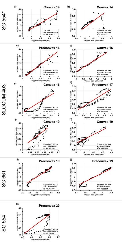
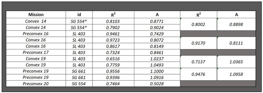
ISTITUTO NAZIONALE di Oceanografia e di Geofisica Sperimentale Trieste

Best fit line using least square minimization of the glider oxygen data

The compensated oxygen values obtained from the glider data were then “calibrated” using the
least square minimization (model Y=X+A, where A has to be optimized) as already done in Gerin
et al. (2020) and Gerin and Martellucci (2020) for the float data (Fig. 19 and Table 5).
The coefficients of determination of the least square minimization are always quite high (6 out of
11 are higher than 0.8; 0.73 is the lowest value).

During the Convex 14 glider mission, performed by the SeaGlider 554 the oxygen data was
“calibrated” using two float profiles. In the first comparison (Fig. 19a) the coefficient of
determination is 0.81 and the A coefficient is equal to 0.87 ml/l, while in the second comparison
the coefficient of determination is 0.79 and the A coefficient increases a little bit to 0.90 ml/l (Fig.
19b). Using both data together, the coefficient of determination is 0.80 and the A coefficient 0.89
ml/l (Table 5).

The Slocum glider 403 was used in several missions. The least square minimization always
evidences an underestimation of the glider oxygen concentration and, generally, a very high
coefficient of determination (R2) between 0.65 and 0.97 and an A coefficient increasing with the
time of usage from 0.74 ml/l to 1.05 ml/l (Figs. from 19c to 19h and Table 5).

The SeaGlider 661 dissolved oxygen sensor was “calibrated” using two float profiles recorded
during the early December 2019 (Figs. 19i and 19j and Table 5).
The oxygen data minimization with the earliest float profile and the glider gives a coefficient of
determination of 0.95 and a A coefficient equal to 1.1 ml/l, while the second occurrence presents
a coefficient of determination of 0.94 and a coefficient A equal to 1.09 ml/l. The use of these data
together displays a coefficient of determination of 0.95 and a coefficient A equal to 1.09 ml/l.

The SeaGlider 554 was used also during the Preconvex 20 glider mission after being factory
calibrated (therefore it was considered as a different unit). The minimization displays a coefficient
of determination of 0.74 and A coefficient equal to 0.50 ml/l (Fig. 19k and Table 5).

Borgo Grotta Gigante, 09/06/2020 Rel. 2020/36 Sez. OCE 11 MAOS Page 25 of 31

ISTITUTO NAZIONALE di Oceanografia e di Geofisica Sperimentale Trieste

Fig.19: Least square minimization between the compensated oxygen glider data and the float data. In the
 legend the A coefficient and the coefficient of determination are reported.
 SG554* is the SeaGlider 554 before the last factory calibration.

Borgo Grotta Gigante, 09/06/2020 Rel. 2020/36 Sez. OCE 11 MAOS Page 26 of 31

ISTITUTO NAZIONALE di Oceanografia e di Geofisica Sperimentale Trieste

 Table 5: Results of the least square minimization between the compensated oxygen glider data and
 the float data. The coefficient of determination (R 2) and the A coefficient are reported. The last two
 columns are referred to the campaign. SG554* is the SeaGlider 554 before the last factory calibration.

Drift of the oxygen sensor with time (Slocum 403 case)
The results of the least fit minimization for the Slocum glider 403 evidence an increase of the A
coefficient over the time (Table 5). The reason for the increase can be attributed to the
degradation of the Optode sensor mounted on the gliders or to a sensor drift. This drift may also
affect the float according to Bushinsky et al., 2016 that reports a ± 0.1% per year, undermining
our method, in which the float data are used as a reference for the “calibration” of the glider
oxygen data. The oxygen float drift is amplified especially when the glider-float minimization is
done a long time after the float “calibration”.

The Slocum 403 was used longer than the other gliders allowing a better analysis of the glider
oxygen drift over time. The A coefficient computed by mission using a set of float oxygen data
provided by sensors with different aging (Table 5), plotted versus time shows a regular increase
over time of +0.1 ml/l per year (Fig. 20). The high regression coefficient of R 2=0.99 of the four
“calibration” versus time suggests that the possible drift of the float oxygen sensor is negligible
with respect to the one mounted on the glider. Indeed, the drift observed is 1 order higher than
the one declared by the Aanderaa.
The fact that gliders are operated in the water only for limited periods and then stored for a long
time might be the reason of the higher observed drift. Despite the standard maintenance of the
Optode sensor after every mission following the Aanderaa TD269 Oxygen Optode operating
manual, (2017) is performed, its membrane tends to dry out and consequently is affected by an
important degeneration.

Borgo Grotta Gigante, 09/06/2020 Rel. 2020/36 Sez. OCE 11 MAOS Page 27 of 31

ISTITUTO NAZIONALE di Oceanografia e di Geofisica Sperimentale Trieste

Fig.20: Regression of the A coefficient for the Slocum glider 403 over time. Red dots are the A coefficient
 as in Table 5; the x axis represents the days after the factory calibration (11 April 2013).

Oxygen drift due to foil: Aanderaa factory indications

The Aanderaa support center notified that in some cases the foil can have a drift of 3 - 8% offset
prior to deployment, and after that stabilized with a drift of about 0.2% per year.
This evidences the importance of our “calibration”, which is about one order higher than
Aanderaa's notification.

Possible correction for the oxygen glider data without a reference
As discussed in the report (e.g.: Fig. 13), it was not possible to “calibrate” the collected glider
oxygen data using the above method during the PreConvex18 (Slocum glider 402), the Convex17
and Convex18 (Slocum glider 403) missions, due to the lack of validated Winkler samples and/or
quality-controlled and Winkler-calibrated oxygen float data close in space and time.
We propose an alternative way to correct the compensated oxygen glider data of the Convex17
and Convex18 using the computed regression (Fig. 20). The estimated coefficients are
summarized in Table 6.
The correction of the PreConvex18 glider data requires an assumption: the membrane (sensing
foil) of the two sensors mounted on 402 and 403 units degraded over time at the same rate. This
assumption is comforted by the calibration certificate that reports the calibration on the same day
(11 April 2013). We can therefore speculate that the regression obtained for the Slocum glider
403 (Fig. 20) can be applied on the glider 402.

Borgo Grotta Gigante, 09/06/2020 Rel. 2020/36 Sez. OCE 11 MAOS Page 28 of 31

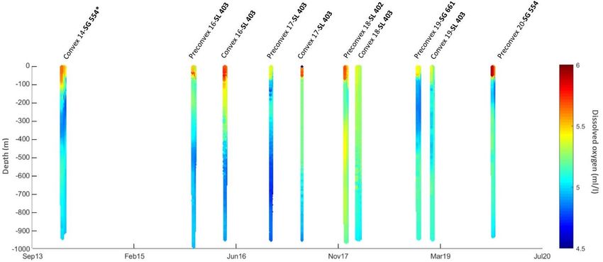
ISTITUTO NAZIONALE di Oceanografia e di Geofisica Sperimentale Trieste

 Table 6: Estimated coefficients for the oxygen calibration for the
 Convex17, Convex18 and Preconvex18 missions.

Final results

All the oxygen glider data were corrected applying the coefficient of Tables 5 and 6. The final
glider dataset (Fig. 21) was compared with the data collected at P-1200 L-term station (Fig. 14)
and at the E2M3A station (not shown) obtaining a very good qualitative agreement.

 Fig. 21: Time series of the “calibrated” and compensated oxygen data of the different glider missions.
 SG554* is the SeaGlider 554 before the last factory calibration.

Acknowledges

The authors would like to acknowledges dr. Kovačević and dr. Bensi for sharing the ESAW-1 and
ESAW-2 data, dr. Cardin for the E2M3A Winkler data and dr. Garić and dr. Batistić for the plot of
the oxygen saturation measured at P-1200 L-term station. It was very useful to understand the
problem and confirm the quality of the “calibrated” glider oxygen data.

Borgo Grotta Gigante, 09/06/2020 Rel. 2020/36 Sez. OCE 11 MAOS Page 29 of 31

ISTITUTO NAZIONALE di Oceanografia e di Geofisica Sperimentale Trieste

References

Aanderaa TD 269 OPERATING MANUAL OXYGEN OPTODE 4330, 4831, 4835, June 2017.

Artegiani, A., Paschini, E., Russo, A., Bregant, D., Raicich, F., & Pinardi, N. (1997). The Adriatic
Sea general circulation. Part I: Air–sea interactions and water mass structure. Journal of physical
oceanography, 27(8), 1492-1514.

Bittig, H. C., Körtzinger, A., Johnson, K. S., Claustre, H., Emerson, S., Fennel, K., et al. (2016).
SCOR WG 142: Quality Control Procedures for Oxygen and Other Biogeochemical Sensors on
Floats and Gliders. Recommendations on the Conversion between Oxygen Quantities for Bio-
Argo Floats and Other Autonomous Sensor Platforms. doi: 10.13155/45915

Bushinsky S.M., Emerson S. R., Riser S.C. and Swift D.D., 2016. Accurate oxygen measurements
on modified Argo floats using in situ air calibrations. Limnology and Oceanography, 14 (8), 491-
505. https://doi.org/10.1002/lom3.10107

Cushman –Roisin B., Gacic M., Poulain P.-M., Artegiani A. (2001). Physical oceanography of the
Adriatic sea, Kluwer Academic Publishers

Garau B., Ruiz S., Zhang W., Pascual A., Heslop E., Kerfoot J. and Tintoré J. (2011). Thermal
Lag Correction on Slocum CTD Glider Data. Journal of Atmospheric and Oceanic Technology
(28), 1065-1071. 10.1175/JTECH-D-10-05030.1

Gerin R., Martellucci R., Notarstefano G. and Mauri E. (2020). Float oxygen data calibration with
discrete Winkler samples in the South Adriatic Sea. REL. 2020/30 OCE 9 MAOS, Trieste, Italy,
21 pp.

Gerin R. and Martellucci (2020). Float 6901865 oxygen data calibration. REL. 2020/35 OCE 10
MAOS, Trieste, Italy, 6 pp.

Manca B., Burca M., Giorgetti A., Coatanoan C., Garcia M.-J. and Iona A., 2004. Physical and
biochemical averaged vertical pro- files in the Mediterranean regions: an important tool to trace
the climatology of water masses and to validate incoming data from operational oceanography,
J. Marine Syst., 48, 83–116, https://doi.org/10.1016/j.jmarsys.2003.11.025.

Queste, B.Y., Heywood, K.J., Smith, W.O., Kaufman, D.E., Jickells, T.D., & Dinniman, M.S., 2015.
Dissolved oxygen dynamics during a phytoplankton bloom in the Ross Sea polynya. Antarctic
Science, 27, 362-372.

Šantić D., Kovačević V., Bensi M., Giani M., Vrdoljak A., Ordulj M., Santinelli C., Šestanović S.,
Šolić M. and Grbec B., 2019. Picoplankton Distribution and Activity in the Deep Waters of the
Southern Adriatic Sea. Water, 11, 1655.

Borgo Grotta Gigante, 09/06/2020 Rel. 2020/36 Sez. OCE 11 MAOS Page 30 of 31

ISTITUTO NAZIONALE di Oceanografia e di Geofisica Sperimentale Trieste

Strickland, J.D.H., and Parsons, T.R. (1968). Determination of dissolved oxygen. in A
Practical Handbook of Seawater Analysis. Fisheries Research Board of Canada,Bulletin,
167, 71–75.

Uchida H., Kawano T., Kaneko I. and Fukasawa M. (2008). In Situ Calibration of Optode-Based
Oxygen Sensors. Journal Of Atmospheric and Oceanic Technology (25), 2271-2281.

Winkler, L.W. (1888). Die Bestimmung des in Wasser gelösten Sauerstoffen. Berichte der
Deutschen Chemischen Gesellschaft, 21: 2843–2855.

Zavatarelli M., Raicich F., Bregant D., Russo A. and Artegiani A., 1998. Climatological
biogeochemical characteristics of the Adriatic Sea. J. Mar. Syst. 18, 227–263.

Internet References

 ● http://www.aanderaa.com/media/pdfs/oxygen-optode-4330-4330f.pdf

 ● http://www.seabird.com/document/an64-sbe-43-dissolved-oxygen-sensor-background-
 information-deployment-recommendations

 ● http://www.seabird.com/sbe43-dissolved-oxygen-sensor

 ● https://serc.carleton.edu/microbelife/research_methods/environ_sampling/oxygen.html

 ● http://www.xylemanalytics.co.uk/media/pdfs/aanderaa-oxygen-optode-4831-4831f.pdf

 ● http://www.xylemanalytics.co.uk/media/pdfs/4330-4330f-oxygen-optode_dec12.pdf

Borgo Grotta Gigante, 09/06/2020 Rel. 2020/36 Sez. OCE 11 MAOS Page 31 of 31