Pandemic Meets Pollution: Poor Air Quality Increases Deaths by COVID-19
←
→
Page content transcription
If your browser does not render page correctly, please read the page content below
Discussion Paper Series – CRC TR 224

                                    Discussion Paper No. 262
                                          Project A 02

                     Pandemic Meets Pollution:
           Poor Air Quality Increases Deaths by COVID-19

                                        Ingo E. Isphording 1
                                           Nico Pestel 2

                                            January 2021

                1
                    Institute of Labor Economics (IZA), CESifo, Email: isphording@iza.org
                          2
                            Institute of Labor Economics (IZA), Email: pestel@iza.org

Funding by the Deutsche Forschungsgemeinschaft (DFG, German Research Foundation)
                  through CRC TR 224 is gratefully acknowledged.

                Collaborative Research Center Transregio 224 - www.crctr224.de
             Rheinische Friedrich-Wilhelms-Universität Bonn - Universität Mannheim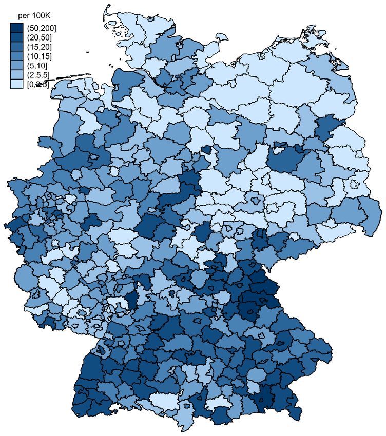
Pandemic meets Pollution:
                        Poor Air Quality increases
                          Deaths by COVID-19*

                             Ingo E. Isphording                     Nico Pestel

                                            January 29, 2021

         We study the impact of short-term exposure to ambient air pollution on the spread and
         severity of COVID-19 in Germany. We combine data on county-by-day level on confirmed
         cases and deaths with information on local air quality and weather conditions. Following
         Deryugina et al. (2019), we instrument short-term variation in local concentrations of
         particulate matter (PM10) by region-specific daily variation in wind directions. We find
         significant positive effects of PM10 concentration on death numbers from four days before
         to ten days after the onset of symptoms. Specifically, for elderly patients (80+ years) an
         increase in ambient PM10 concentration by one standard deviation between two and four
         days after developing symptoms increases deaths by 19 percent of a standard deviation.
         In addition, higher levels air pollution raise the number of confirmed cases of COVID-19
         for all age groups. The timing of effects surrounding the onset of illness suggests that
         air pollution affects the severity of already realized infections. We discuss implications
         of our results for immediate policy levers to reduce the exposure and level of ambient
         air pollution, as well as for cost-benefit considerations of policies aiming at sustainable
         longer-term reductions of pollution levels.

JEL Classification: I12, I18, Q53
Keywords: COVID-19, health, air pollution, Germany

 *
     Ingo E. Isphording: Institute of Labor Economics (IZA), CESifo, Email: isphording@iza.org, Nico Pestel:
      Institute of Labor Economics (IZA), Email: pestel@iza.org. The authors have no financial or other conflicts
      of interest to disclose. Acknowledgements: We are grateful to Steffen Künn, Juan Palacios, Nicolas R.
      Ziebarth, seminar participants at IZA as well as the editor and two anonymous referees for extremely helpful
      comments and suggestions. Dajan Baischew, Eva Justenhoven and Marc Lipfert provided excellent research
      assistance. Funding by the German Research Foundation (DFG) through CRC TR 224 (Project A02) is
      gratefully acknowledged. An earlier version of this paper is available as IZA Discussion Paper No. 13418.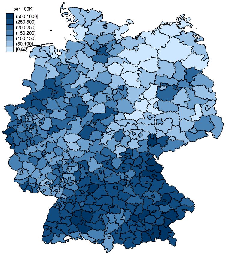
1 Introduction

The novel coronavirus (SARS-CoV-2) has sparked the largest public health and economic crisis
in recent history. Up to date, the coronavirus disease 2019 (COVID-19) pandemic with millions
of confirmed cases has claimed more than 1.5 million deaths globally.1 World Bank projections
of economic damage range up to a 5.2 percent contraction in global GDP, which would be the
deepest recession in decades (World Bank, 2020). Other pressing social and economic issues,
most notably environmental issues of climate change and pollution, have almost vanished from
the public debate and are only slowly re-emerging.

        In this paper, we show that both environmental pollution and the COVID-19 pandemic
are significantly connected: higher levels of local air pollution increase the number of deaths
of COVID-19, leading to a more severe course of the pandemic. Three plausible mechanisms
link air pollution to the spread and course of severe acute respiratory infections (SARI) and
influenza-like illnesses (ILI). First, long-run exposure to air pollution is linked to medical pre-
conditions such as illnesses of the respiratory system that can exacerbate the course of the
disease (Analitis et al., 2006; Atkinson et al., 2001; Le Tertre et al., 2002; Dominici et al.,
2003; Katsouyanni et al., 2001). Second, short-term exposure to air pollution leads to in-
flammatory reactions and lower immune responses to new infections (Ciencewicki and Jaspers,
2007; Contini and Costabile, 2020; Martelletti and Martelletti, 2020). Third, higher levels of
air pollution increase the ability of viruses for airborne infection by prolonging the time the
virus remains in open air (Cui et al., 2003; Frontera et al., 2020). Whether these mechanisms
are at play in the case of the novel coronavirus remains open to debate.

        Against this background, we add to the epidemiological literature empirically linking
levels of different air pollutants to the onset and severity of SARI and ILI in general, and
the new COVID-19 disease specifically. We study the interaction of short-term exposure to
ambient air pollution, measured by levels of particulate matter (PM10) in German counties,
and the number of newly confirmed cases and deaths of COVID-19. We instrument levels
of PM10 by exploiting region-specific relationships between wind direction and air pollution
following Deryugina et al. (2019). Fixed effects for county and date keep county-specific
time-invariant and national time-variant confounding variables constant. We further control
for several potentially confounding variables: weather conditions, the county-specific state
of the pandemic, local mobility patterns based on mobile phone movements, county-specific

 1
     Numbers taken from the John Hopkins University Coronavirus Resource Center: https://coronavirus.
     jhu.edu/map.html (last updated: 11 December, 2020).

                                                  1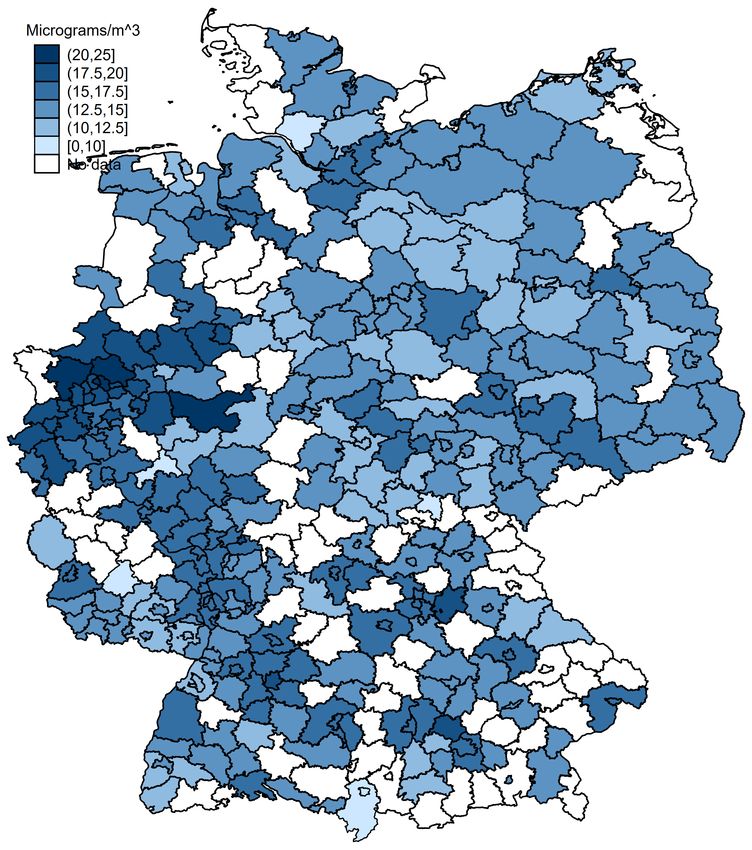
requirements for wearing face masks in public as well as state-specific fixed effects for the
different policy regimes implemented in response to the first wave of the pandemic between
spring and early summer of 2020 in Germany.

      We find significant effects of higher air pollution on both the number of deaths as well
as the number of confirmed cases by day and county. Effects are specifically pronounced for
patients aged 80 and above. For this age group, significant effects of air pollution arise for
male patients from four days before to ten days after the onset of symptoms. A one standard
deviation increase in the three-day average PM10 concentration (7.2 µg/m3 ) over the period
between two and four days after the onset of illness increases the number of deaths among male
patients by about 1.2 deaths per 100K population per day or about 19 percent of a standard
deviation. Effect patterns for women are similar, yet less pronounced. Additionally, we find
that air pollution just before as well as after the onset of illness leads to increased numbers
of confirmed cases across the entire age distribution which is likely explained by aggravated
symptoms swaying patients to get tested.

      By isolating the causal effect of air pollution on the severity of COVID-19, we comple-
ment and confirm earlier descriptive evidence based on cross-sectional and time-series variation
(see Bhaskar et al. (2020) for a systematic review). To the best of our knowledge, there are few
studies estimating quasi-experimental causal links between air pollution and ILI or respiratory
disease severity. Clay et al. (2018) exploit differential timing of the Spanish flu pandemic across
U.S. cities to show that contemporary short-term air pollution levels increased the number of
deaths. Moghadas et al. (2020) show that US county-by-month influenza-related hospital-
izations increase with higher air pollution. Persico and Johnson (2020) show with respect
to the COVID-19 pandemic that air pollution, instrumented by a rollback of environmental
regulations in the U.S., increases both cases and case fatality of COVID-19. Also for the U.S.,
Austin et al. (2020) apply the same IV approach using county-level variation in wind directions
to study the impact of fine particle concentrations on cases and deaths of COVID-19.

      We add to these more closely related papers in two important ways. First, whether or
not results from previous pandemics and/or other regional settings are generalizable to other
external settings, both in case of disease and locality, is yet to be determined. To the best
of our knowledge, we are the first to provide evidence on the linkage between air pollution
and the spread as well as the severity of COVID-19 for Germany. Second, we use fine-grained
data on daily pollution levels which allow us to identify critical time windows relative to the
onset of the illness when pollution levels most crucially affect the mortality risk. This allows

                                                2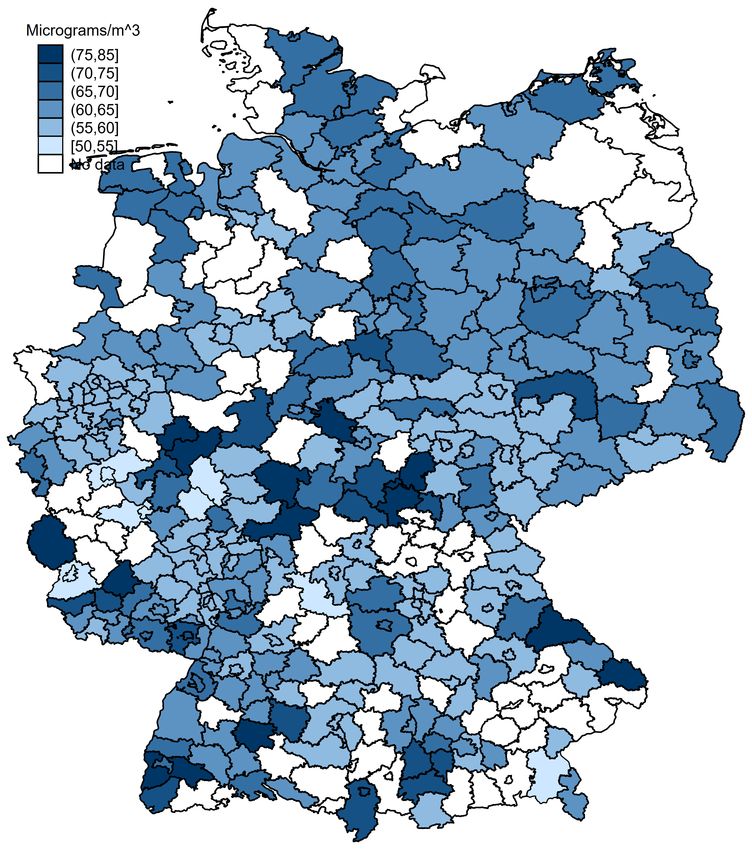
us to discriminate between different mechanisms at play. As effects materialize just before
and mainly after the onset of illness, our results support mechanisms causing inflammatory
reactions, reducing the immune response and aggravating symptoms. Our results do not
support proposed mechanisms of higher ability of the virus for airborne infections due to higher
air pollution. By focusing on short-term changes in the exposure to air pollution, our results
do not speak to potential effects through longer-run exposure to air pollution on respiratory
preconditions.

         We discuss three groups of policy instruments that may be justified by the results of
this paper: first, any policy that reduces the exposure of vulnerable patients towards ambient
air pollution might lead to a reduced mortality of COVID-19. Second, policies that directly
reduce levels of air pollution should be considered. Third, our results confirm that policies
sustainably reducing pollution levels will have substantial health effects through lower severity
of respiratory diseases.

         The remainder of this paper is organized as follows. Section 2 discusses plausible mech-
anisms through which higher air pollution might affect onset and severity of COVID-19 and
summarizes the related literature. Section 3 describes the data and provides a descriptive
overview on the course of the pandemic in Germany. Section 4 describes our empirical ap-
proach. Section 5 presents the main results as well as additional analyses. Section 6 discusses
implications for policy-makers. Section 7 concludes.

2 Background and Literature

Mechanisms. The medical literature has analyzed a number of direct physiological mecha-
nisms how acute air pollution could affect the infection probabilities and severeness of respi-
ratory virus infections, such as influenza and SARS (see Ciencewicki and Jaspers, 2007, for
a review). Several authors speculate that these mechanisms could be at play in the case of
COVID-19 (Contini and Costabile, 2020; Martelletti and Martelletti, 2020).

         Direct physiological mechanisms range from lower initial immune response, reduced abil-
ity of macrophages (cells specialized in the detection and destruction of harmful organisms,
including viruses), and stronger oxidative stress.2 Specific to particulate matter (PM) concen-
tration, mice display lower early immune responses when having been exposed to carbon black
particles (Lambert et al., 2003). PM-exposed macrophages display lower abilities to devour
 2
     Oxidative stress describes a situation where the production of free radicals exceeds the metabolism’s ability
     to counteract or detoxify and contributes to the pathogenesis of respiratory infections (Liu et al., 2017).

                                                         3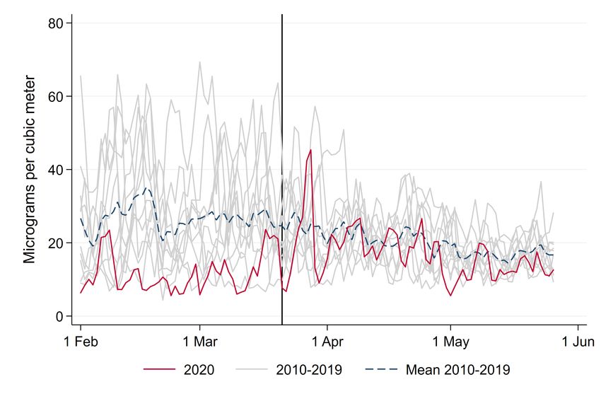
viruses (Kaan and Hegele, 2003; Becker and Soukup, 1999). Several lab studies show that
animals or cell cultures develop stronger oxidative stress and aggravated disease severity after
being exposed to PM (Jaspers et al., 2005; Lee et al., 2014).

      A second type of mechanisms is related to how air pollution is affecting the airborne
transmission of viruses. A number of studies suggests that higher levels of air pollution,
especially PM concentration, increase the ability of viruses for airborne infection and raise the
initial viral load (Cui et al., 2003; Frontera et al., 2020). With respect to SARS-CoV-2 it has
been shown that the infectious dose and the initial viral load is an important predictor for the
severeness of cases (Zheng et al., 2020).

      Besides these acute direct effects, air pollution has repeatedly been shown to be strongly
linked to medical pre-conditions such as cardiovascular and respiratory diseases that have been
found to crucially affect the severeness of COVID-19 (Analitis et al., 2006; Atkinson et al.,
2001; Le Tertre et al., 2002; Dominici et al., 2003; Katsouyanni et al., 2001). As we focus in
our empirical analysis on the effect of short-term changes in the exposure to pollutants, these
long-term effects are not the focus of this study.

Epidemiological evidence. Tracing the outcome of these mechanisms in the field, a number
of epidemiological studies proposes empirical links between measures of air quality and case
numbers and deaths of respiratory virus infections. With few exceptions, the majority of these
studies rely on either pure cross-sectional or regional time series variation. Both approaches
limit opportunities to identify a causal link due to potential confounders on both the time and
regional level. Spatial variation likely correlates with the presence of obvious confounders, such
as population density, public transport usage and age composition. Variation in air pollution
over time might be plagued by simultaneity and reversed causality issues. For example, several
studies have shown that the reduced economic activity that follows an outbreak has strong
effects on air pollution – an obvious challenge for the estimation of a causal effect of the latter
on the former.

      Based on cross-sectional variation, a positive link between regional air pollution and the
local severeness of the COVID-19 pandemic and related severe acute respiratory and influenza-
like virus infections has been shown. For the early and severely hit region of Northern Italy,
several cross-sectional studies propose a relationship between high levels of air pollution and
COVID-19 cases (Contini and Costabile, 2020; Pansini and Fornacca, 2020). Others have raised
concerns that the high level of domestic bio mass fuel usage in developing countries might

                                                4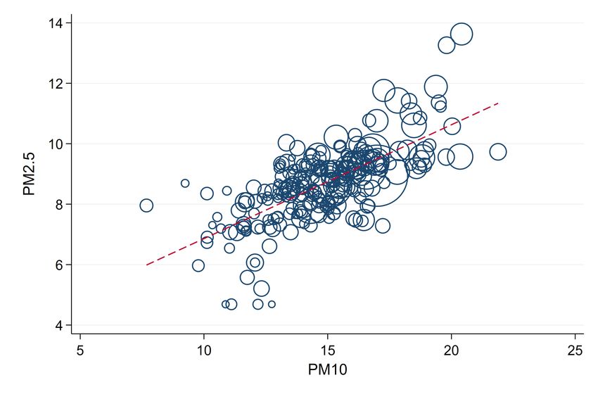
aggravate the impact of the pandemic (Thakur et al., 2020) – an effect that was already
foreshadowed by evidence from the interaction of biomass fuel usage and the Spanish flu
pandemic (Clay et al., 2018). For countries besides Italy, Andree (2020) and Cole et al. (2020)
report correlations between air pollution and COVID-19 cases across Dutch municipalities.
Travaglio et al. (2020) finds positive associations between markers of poor air quality and
COVID-19 cases in England. For China, Yongjian et al. (2020) and Yao et al. (2020) describe
positive spatial associations between PM2.5 and PM10 and COVID-19 death rates. Wu et al.
(2020) find that small increases in long-term PM2.5 concentration are associated with large
increases in the COVID-19 death rate, yet acknowledging the inherent limitations of their study
design.

      Other studies focus on (regional) time series variation in PM. Several studies show
positive time series correlations between daily PM levels and influenza-like illnesses in Chinese
regions (Liang et al., 2014; Su et al., 2019; Huang et al., 2016). Chen et al. (2018) show
Granger causality between PM2.5 and weekly influenza cases with specifically strong effects
on the elderly. Similar relationships have previously been found for SARS (Cui et al., 2003).

Causal Effects of Air Pollution.     Few studies have attempted to identify a causal effect of
air pollution on the onset and severity of respiratory infections using quasi-experimental study
designs. Clay et al. (2018) show that air pollution exacerbated the impact of the Spanish
flu by applying fixed effects regressions exploiting the differential timing of the pandemic
across U.S. cities. Based on a similar methodological approach as our own, Moghadas et al.
(2020) show that county-by-month influenza-related hospitalizations increase with higher air
pollution. Persico and Johnson (2020) show with respect to the COVID-19 pandemic that air
pollution, instrumented by a rollback of environmental regulations, increases both cases and
case fatality of COVID-19 in the U.S. In a closely related paper, Austin et al. (2020) also apply
an instrumental variable approach exploiting daily variation in regional wind direction following
Deryugina et al. (2019) using county-level data from the U.S. and also find that higher PM2.5
concentrations increase confirmed cases and deaths of COVID-19.

3 Data and Descriptives

COVID-19 cases and deaths.         We collect data on confirmed cases and deaths of COVID-
19 by German counties (Kreise) from the official German COVID-19 reporting database by
the Robert-Koch-Institut (RKI). In accordance with the Infection Protection Act (Infektionss-

                                               5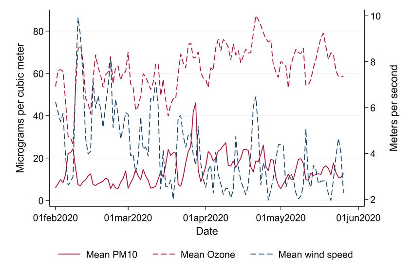
chutzgesetz), the RKI collects daily reports from county-level public health offices on newly
detected cases and deaths. Case reports are transmitted to the RKI by 0:00 a.m. on the
respective day. The records contain the exact date on which the local public health office
became aware of the case and recorded it electronically. For most cases, the data contains
additional information on when the patient became ill with clinical symptoms according to the
patient’s own statement or according to the statement of the treating physician (illness onset).
Cases are separately recorded by gender and age group (0–34, 35–59, 60–79, 80+). Daily case
counts are regularly updated based on delayed lab confirmations and deaths of earlier recorded
cases. The analysis of this paper is based on a snapshot of the data taken on May 26, 2020.
We use population counts of demographic groups to normalize case numbers and deaths to
100K inhabitants by county, gender and age.

        Table 1 displays average day-by-county cases and deaths per 100K population, as well
as cell population shares for gender × age groups over the entire window of observation
from February 1 until May 26, 2020. The bottom row displays average cases and deaths
across all age × gender groups. On average, we observe 1.73 confirmed cases and 0.09
deaths per day per county, a case fatality rate (i.e., the probability of dying of COVID-19
conditional on being a confirmed case) of 5.2 percent. Germany’s comparably low case fatality
rate compared to European hotspots such as Spain (14.5 percent) or Italy (11.5 percent)3
has been explained by several arguments: higher numbers of intensive care beds, higher test
intensity and demographic factors such as a younger population living largely separated from
their parent’s generation (Bayer and Kuhn, 2020).

        There is considerable heterogeneity in the number of deaths and confirmed cases by age
and gender. Below age 80, case prevalence varies little by age and gender between 1.3 and 2.2
cases per 100K population in a respective demographic group. Only among the very old aged
80 and above we observe a higher prevalence of 2.86 cases per 100K population for males and
of 3.11 cases for females. Deaths due to COVID-19 are also concentrated among the very old.
Below age 60, we observe close to zero deaths per 100K per demographic group. Among male
patients between 60 and 79 we observe 0.19 daily deaths per 100K population. The resulting
case fatality rate in this demographic group is about eleven percent. Female patients of the
same age group display a significantly lower case fatality rate of just 5.1 percent. For very
old patients above 80 years, deaths are substantially higher: per 100K population, we observe
about one death per day per county for male and about 0.74 deaths per day per county for

 3
     Fatality rates are from https://ourworldindata.org/coronavirus/ (last accessed June 23, 2020).

                                                    6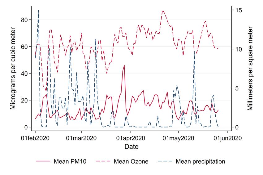
Table 1: Descriptives: COVID-19 cases and deaths (by county and day)
                            Cases per 100K               Deaths per 100K                 Pop. share

 Age range    Gender      Mean           SD             Mean          SD          Mean                SD

 0–34         Men         1.28           3.56             0          .03           .19                .02
 0–34         Women       1.39           3.42             0           .03          .17                .02
 35–59        Men         1.91          4.28            .02           .25          .18                .01
 35–59        Women       2.17           4.69            .01         .16           .17                .01
 60–79        Men         1.67          4.57            .19          1.28          .11                .01
 60–79        Women       1.37           3.89            .07         .65           .12                .02
 80+          Men         2.86          11.55           1.04         6.14          .03                 0
 80+          Women       3.11          13.52           .74          4.77          .04                .01
 All          All         1.73           3.14           .09           .36           1                  0

Notes: This table summarizes means and standard deviations of confirmed cases and deaths of COVID-19, as
well as average population shares of demographic groups separated by age and gender. All numbers averaged
across counties. Source: RKI and Statistical Office.

female patients. Associated case fatality rates are 36 percent for male and 24 percent for
female patients.

         To understand the limits of interpretation of the data, it is important to discuss the
testing regime that has been in place over the period under consideration. COVID-19 cases are
confirmed after a patient has been positively tested. During the peak of the pandemic, patients
in Germany mostly were eligible for scarce testing capacities after having developed symptoms
(acute respiratory symptoms and/or loss of sense of taste/smell) or after having been in contact
with a confirmed case. Thus, it can be expected that the majority of asymptomatic cases will
have remained undetected. Early estimates of the share of symptomatic cases based on Chinese
data of the City of Wuhan range from 5 to 9.2 percent (Read et al., 2020; Nishiura et al.,
2020). A population study in the county of Heinsberg in North Rhine-Westphalia, Germany,
estimates a 5-fold higher number of infected individuals than the number of officially reported
cases (Streeck et al., 2020).

Timeline of the pandemic.          First cases of COVID-19 in Germany were registered and con-
tained near Munich, Bavaria, at the end of January 2020. After that, only on February 25
additional cases, which were related to the outbreak in Italy, were detected in in the state of
Baden-Wuerttemberg. A first major cluster emerged at the beginning of March in the county
of Heinsberg in the state of North Rhine-Westphalia. Shortly after, additional clusters broke
out all over the country. German disease control initially reacted by local containment strate-
gies, and federal and state governments stressed that the country was well prepared for a larger

                                                    7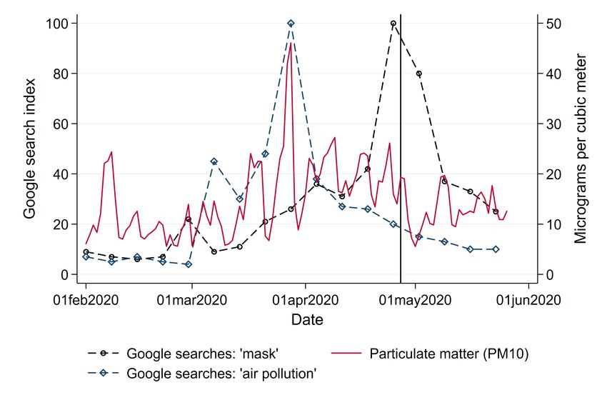
outbreak.

      On March 11, 2020, on the day the World Health Organization announced the pandemic
status of the Corona outbreak, Chancellor Angela Merkel asked the German population to do
anything to avoid the further spread of the virus. Schools and public child care as well
as national borders were closed on March 15. On March 16, closures of bars, restaurants,
churches and shops followed. Federal states reacted with severe mandatory social-distancing
measures from March 21 onward. Groups outside were restricted to no more than two persons
if from different household. In some states leaving one’s home was only allowed for important
or recreational activities. From March 30 onward, visits to hospitals and homes for elderly were
prohibited. After numbers of newly infected decreased again, counter-measures were slowly
retracted starting on April 15.

      Figure 1 summarizes the course of the pandemic over our window of observation from
February to May 2020. Registered cases are displayed in light-blue, deaths in dark-blue bars.
Until June 8, 184,193 cases, 8,674 deaths and about 169,600 recoveries were reported to the
RKI. The pandemic has hit German regions differentially. Figure A.1 in the Appendix shows
the total number of confirmed cases and deaths per 100K of population as of May 26, 2020.
Following first clusters that had emerged in the states of North Rhine-Westphalia, Bavaria
and Baden-Wuerttemberg, these states remained the hotspots of the pandemic. Northern and
especially Eastern states (with the exception of the city of Berlin) were hit much less severely,
with some counties up to beginning of June experiencing less than 50 cumulative cases per
100K population.

Air pollution. We assess local levels of air pollution by particulate matter (PM) which
measures the concentration of small airborne particles including dust, dirt, soot, smoke and
liquid droplets. PM may be emitted by natural sources such as bush fires, dust storms,
pollens and sea spray, or anthropogenic (“man-made”) sources like motor vehicle emissions
and industrial processes.

      In our main empirical analysis, we focus on PM10, i.e., the concentration of particles
up to a diameter of 10 µm. We later corroborate our results using PM2.5. Unfortunately, the
coverage of PM2.5 measurements in Germany is significantly scarcer than for PM10. For the
window of analysis, measurements of these smaller particulates are only available for a selective
set of counties. Both measures are highly correlated and lead to similar aforementioned physical
reactions of the human body. Levels of PM10 are highly correlated to levels of further pollutants

                                               8
Figure 1: Daily variation in new confirmed cases and deaths and mean air pollution
Note: This graph shows the total number of new confirmed cases and deaths of COVID-19 in Germany as well as the
mean concentration of particulate matter (PM10) and ozone (O3) by date. Source: RKI and UBA.
such like NO2, SO2 and CO which are associated to similar inflammatory reactions. Yet, these
pollutants are less well covered by measurement stations.
In addition, we assess levels of ozone (O3) as a second dimension of air pollution.
Ozone levels are in general negatively correlated to PM levels, yet they again lead to similar
inflammatory reactions (Ciencewicki and Jaspers, 2007). Ozone arises from reactions under
sunlight of nitrogen oxide with so-called ’reactive organic substances’. These substances mainly
stem from motor vehicle exhaust and aviation. As we focus on the effect of PM10, we treat
ozone as a confounder in our regressions. We separately show patterns of the effect of ozone
on onset and severity of the disease in the additional analyses in the Appendix.
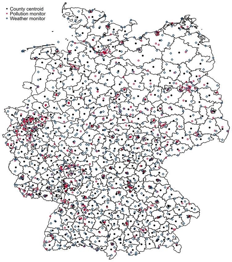
Data on PM10 and O3 are provided on a daily basis by the air pollution monitoring system
of the German Federal Environment Agency (Umweltbundesamt, UBA). Data is available on
the geo-coded monitor level which allows us to assign levels of air pollution to counties.
Specifically, we compute a county’s daily pollution level as the inverse-distance weighted mean
of all monitors within a radius of 25 km around the county centroid as a proxy for the population
center. Figure A.2 displays the coverage of counties through monitors.
9Table 2 summarizes county-levels of daily and three-day averages of air pollution. All
pollutants are measured in units of µg/m3 . As in the case of confirmed COVID-19 cases
per population, Figure A.3 in the Appendix shows strong heterogeneity in air pollution across
counties. PM10 is closely associated with industry agglomeration and population density, with
highest levels in Western Germany, concentrated in the highly populated and industrialized
regions in North Rhine-Westphalia, Rhineland-Palatinate and Baden-Wuerttemberg following
the rivers Rhine, Main and Ruhr which connected the former heavily industrialized regions
of Western Germany. Interpreting simple spatial correlations between average levels of air
pollution and local onset and severity of the COVID-19 pandemic might lead to erroneous
claims about a causal effect of the former on the latter. We will instead focus in our empirical
analysis on within-county changes in short-term exposure to air pollution to circumvent this
identification problem.
Solid and dashed red lines of Figure 1 display average levels of our main independent of
interest: levels of PM10 and O3. Both variables display significant day-to-day variation over
time. While PM10 pollution levels have in general declined by the reduced economic activity
during the pandemic (Venter et al., 2020), we do not observe respective reductions in Germany.
Rather, levels of PM10 even reached a maximum during the peak of the crisis. Reasons for this
particular development of air pollution in Germany lie in several sources. First and foremost,
the lockdown coincided with a period of extremely low precipitation, reducing the amount of
PM washed out of the air by rain (see below). Second, the German lockdown was less severe
than lockdowns in other countries. While economic activity was reduced overall, economic
sectors being hit hardest by the lockdown, such as the hospitality, entertainment industry and
retailing, are characterized by rather low levels of emissions. Strongly polluting industries in
the manufacturing sector kept up their production during the lockdown. Industrial processes,
heating and agriculture arguably less affected by the lockdown contribute up to about 70
percent.4 Taken together, these facts led to for German standards above average levels of
pollution during the lockdown as can be seen from Appendix Figure A.4 which depicts pollution
levels in Spring 2020 compared to pollution levels over the past ten years.
Weather. Weather conditions drastically changed in Germany almost simultaneously to the
lockdown, leading to particularly high levels of pollution. Levels of air pollution are heavily
4
Calculations based on https://www.umweltbundesamt.de/daten/luft/
luftschadstoff-emissionen-in-deutschland#ermittlung-der-emissionsmengen (last accessed:
June 22, 2020).
10Table 2: Descriptives: Air pollution and weather (by county and day)
Mode of Transport Unit Avg. Period Mean SD Min Max
Air pollution PM10 µg/m3 1 day 14.5 8.5 1 95
PM10 µg/m3 3 days 14.5 7.2 1 55.3
Ozone µg/m3 1 day 62.3 14.8 2.1 132.5
Ozone µg/m3 3 days 62.3 12.8 2.3 125.8
PM2.5 µg/m3 1 day 8.7 5.5 .4 50.6
PM2.5 µg/m3 3 days 8.7 4.6 .7 41.1
Weather Precipitation mm/m2 1 day 2 3.9 0 52.1
Wind speed m/s 1 day 4.1 2 .9 16.5
Temperature ◦ C 1 day 8.4 4.3 -3.5 20.8
Notes: This table summarizes means and standard deviations of average pollution and weather measures
across counties. Source: UBA and DWD.
influenced by local weather conditions. Wind speed and precipitation reduce the level of air
pollution by “washing away” particulate matter. Wind speed and precipitation may also have
a direct effect on the virus spread by affecting contact probabilities and virus survival in the
air, hence we control for these variables as potential confounders. We use daily local mea-
surements of weather conditions provided by the German Meteorological Services (Deutscher
Wetterdienst, DWD) as controls in our regressions. Daily county means of weather conditions
(precipitation in mm/m2 , windspeed in m/s and temperature in degree Celsius) are listed
in Table 2. Figures A.5 and A.6 in the Appendix highlight how both average precipitation
and wind speed dropped to extremely low levels over the entire observation window, partially
explaining the high levels of air pollution coinciding with the pandemic.
Mobility patterns. As several studies have shown by now, the reduced economic activity
during the lockdown has triggered lower levels of air pollution and simultaneously will have led
to lower numbers of cases. To estimate the effect of air pollution in light of these simultaneous
effects, we keep mobility patterns constant by controlling for mobile phone mobility. We use
commercial data on daily levels of mobile phone mobility provided by Teralytics allows to
measure daily frequencies of trips within and across counties of about one third of Germany’s
mobile phone market. Figure A.7 in the Appendix displays the sharp reduction of mobility
during the lockdown.
4 Empirical Approach
To estimate the effect of higher air pollution levels on COVID-19 case numbers and deaths,
we compare changes in case and death numbers in relation to changes in short-term exposure
11to air pollution. To account for potential issues of simultaneity through lockdown measures
affecting both cases and pollution, we instrument local changes by regional effects of wind
directions on pollution. Our aim is to estimate the following relationship:
COVIDgit = αi + µt + βl P M i,t−l + γl Wi,t−l + δl Xi,t−l + εit , (1)
where COVIDgit is the dependent variable, i.e., deaths or confirmed cases in county i for date
of illness onset t, normalized to 100K of population by gender-age group g. Fixed effects for
the county (αi ) and date (µt ) keep time-invariant confounding variables on the county level
and nation-wide homogeneous time-variant factors constant.
Our main independent variable of interest is a three-day average of particulate matter,
P M i,t−l , measured in lags or leads l relative to date of illness onset t.5 We consider lags and
leads about two weeks before and after the date of illness onset to analyze at which stages of
the disease air pollution has an effect on the severity of COVID-19. This window of lags and
leads encompasses the typical course of the disease: The median incubation period between
infection and onset of illness has been reported to range between five to six days (WHO, 2020).
Several studies report a median time between onset of illness until hospitalization of four days
(Docherty et al., 2020; Chen et al., 2020). The time between hospitalization and intensive
care is estimated as about one day (ISARIC, 2020). Other studies report the median time
between onset of illness and pneumonia by four days, and by eight days for acute lung failure
(Guan et al., 2020; Li and Ma, 2020). Based on data from New York, on average, deceased
patients were hospitalized for nine days (Cummings et al., 2020).6
We remain ex ante agnostic about when exactly to expect the effects during the course
of the illness.7 For the number of deaths, plausible effects could happen both during and
before the onset of the infection. Higher initial viral loads, e.g., through higher ability of the
virus for airborne infection at high levels of air pollution, have been shown to lead to more
severe progressions later in the course of the disease. But also effects after the onset of illness
5
Defining lags and leads based on daily changes or longer five-day averages lead to qualitatively similar patterns
(Appendix Figures A.16 to A.19).
6
See also the SARS-CoV-2 briefing note of the RKI at https://www.rki.de/DE/Content/InfAZ/N/
Neuartiges_Coronavirus/Steckbrief.html (last accessed: June 26, 2020).
7
This sets us apart from a common event study design since we cannot rely on a pre-treatment period as
comparison group, as we do not ex ante know when the treatment occurs. Instead, we use as comparison
period time windows where no effect is yet to be expected (before infection) or no more expected (after the
illness).
12are plausible, when higher air pollution causes inflammatory reactions and causes additional
burden for already stressed immune systems, increasing the severeness of symptoms.
For the number of cases, at a first glance it appears only plausible to expect effects up to
the date of onset of illness (the latest point where an infection could have happened), but not
after. Yet, the incomplete testing that hampers the data collection allows for a less obvious
channel of air pollution affecting the number of cases even after their onset of illness: as case
confirmations rely on infected individuals to seek testing, symptoms aggravated through air
pollution after infection and onset of illness can plausibly lead to higher confirmed cases.
In regression model (1), we control for a number of confounding variables for air pollu-
tion as well as factors that affect the dynamics of the epidemic. In particular, we control for
three-day averages of local weather conditions Wi,t−l (temperature, wind speed, precipitation).
In addition, Wi,t−l contains three-day averages of ozone as a potential confounding variable.
While the concentration of particulate matter is typically strongly and positively correlated with
other criteria air pollutants (like nitrogen oxides, sulphur dioxide, carbon monoxide, etc.) and
therefore measurements of PM pick up variation in these other pollutants as well, the correla-
tion of PM and ozone is typically negative as ozone is generated from the chemical interaction
of nitrogen oxides, volatile organic compounds (VOCs) under heat and sunlight. Therefore,
ozone is typically very high in summer when concentrations of PM and other fossil-fuel related
air pollutants are typically lower. Hence, ozone concentrations are typically negatively corre-
lated with PM. Since ozone also irritates the respiratory system of the human body and may
also make COVID-19 more severe, it acts as a confounding variable in the PM analysis which
we keep constant.
Additional control variables are represented by the vector Xi,t−l . To further control
for differing local states of the pandemic as well as local counter-measures, this includes the
number of active cases as the aggregate number of new confirmed cases net of confirmed
deaths over the past three weeks. To control for potential confounding effects of avoiding
behavior through masks (see the later discussion in Section 5.2), we control for local mask
requirements in public transport and shops at the county level collected by Mitze et al. (2020).
Finally, to keep mobility patterns potentially coinciding or triggering reductions in air pollution
statistically constant, we control for several mobility indicators based on mobile phone mobility
as described in Section 3. The vector Xi,t−l also represents controls for county-specific mobility
based on mobile phone data. We also include state-specific fixed effects for the main phases
13of the pandemic throughout the period under investigation.8 Standard errors εit are clustered
at the county level.
The ambient concentration of particulate matter may be endogenous when lockdown
measures, reduced economic activity and social distancing have simultaneous effects on both
COVID-19 case numbers and air pollution. We therefore employ an instrumental variable
approach exploiting plausibly exogenous local variation in wind directions. Wind direction may
serve as a strong predictor of levels of pollution as particles may be transported in ambient air
over long distances. Hence, depending on the wind direction, a location may be more or less
exposed to air pollution stemming from specific sources. On the other hand, wind direction
are plausibly exogenous to severity and case numbers of COVID-19. This IV strategy closely
follows the recent contribution by Deryugina et al. (2019).
We use data from the DWD and assign three-day averages of wind directions at the
county level, W indDiri,t−l , by taking the wind direction measured at the nearest wind monitor
to the county centroid and transform wind direction into four wind direction bins d defined
according to the four quadrants of a wind rose: North-East, South-East, South-West and
North-West. Our instrumental variable is a series of binary indicators resulting from interactions
with the four wind direction bins d and a binary indicator for county i being part of region r.
Regions are defined as federal states, where out of all 16 states the three city-states Berlin,
Hamburg and Bremen as well as the small state of Saarland are merged with their larger
neighboring states, yielding twelve regions in total. Using the most frequent wind direction
bin (South-West) as the baseline, this gives us (D − 1) × R = 3 × 12 = 36 indicator variables
that we use as instruments for P Mi,t−l . Hence, the first stage regression equation reads:
R X
D
φr,d
X
P M i,t−l = l 1(W indDir i,t−l = d) × 1(Regioni = r)
r=1 d=1 (2)
+αi + µt + γl Wi,t−l + δl Xi,t−l + ηit .
This flexible specification allows us to remain agnostic about which wind direction causes
higher air pollution in a specific region, which may depend on the relative direction of major
pollutant sources. Figure A.8 in the Appendix summarizes the results of the first stage.
Grey bars indicate relative frequencies of wind directions which are more or less homogeneous
across regions. During the window of observation, wind from the South-West was the most
8
The main phases are (1) before the national lockdown with comprehensive social distancing requirements
were implemented on 21 March, (2) the lockdown phase from 22 March to 3 May and (3) the phase of
relaxation of social distancing requirements after 3 May.
14common wind direction. Effects of wind direction on pollution differ strongly between regions.
For example, wind from North-East and North-West reduce levels of particulate pollution in
the northern coastal states of Schleswig-Holstein/Hamburg (SH/HH), Niedersachsen/Bremen
(NI/HB) and Mecklenburg-Vorpommern (MV), as it transports relatively clean air from the
North and Baltic Sea. In other states, the same wind direction leads to higher air pollution
relative to days with the wind blowing from the South-West as it carries particles suspended
from inland emission sources.
5 Results
5.1 Effects of PM10 on COVID-19 cases and deaths
Effect of PM10 on deaths. Figure 2 displays coefficients of three-day averages of PM10
for lags and leads surrounding the day of onset of illness on the number of deaths per 100K
population in a respective demographic group. The estimation is based on equation (1).
Each coefficient stems from a separate regression of the number of deaths in a particular age
and gender group on the respective lag/lead predicted pollution levels. Pollution appears to be
unrelated to the severity of the pandemic if it occurs before infection. From four days before the
onset of symptoms, higher levels of PM10 display significant effects which are heterogeneous
by age group.
For patients below 60, effect patterns are precisely estimated and remain close to zero.
For male patients aged 60–79 years, we observe significant effects from the onset of illness
onward, with highest effects just after symptoms occurred: A one µg/m3 increase in PM10
two to four days after onset of illness leads to 0.042 additional deaths per 100K population.
Translated to standard deviations as reported in Tables 1 and 2, a one standard deviation
increase in air pollution two to four days after the onset of illness leads on average to 0.3
additional deaths per 100K population. This effect is sizable in relative terms and accounts for
an increase of about 24 percent of a standard deviation of the fatality rate of this demographic
group. For women, the effect is similar in relative terms, but is only marginally significant with
an effect of about 0.01 additional deaths for a one µg/m3 increase in PM10 two to four days
after the onset of symptoms.
For men aged 80 years and older, we observe significant positive effects from four days
before to 10 days after the onset of symptoms. The effect is largest between five and seven
days after the onset of illness. At this point a one µg/m3 increase in PM10 leads to about
15Figure 2: Effect of PM10 on new deaths from COVID-19
Note: This graph shows the point estimates and the 95 percent confidence intervals of the effect of PM10
concentration on the number of deaths per 100K population from COVID-19. Each coefficient results from a separate
regression of deceased patients on the respective lag/lead of predicted levels of PM10 relative to the onset of illness.
Source: RKI, UBA and DWD.
0.16 additional deaths per 100K population. This implies an effect of a one standard deviation
increase in air pollution of 1.2 additional deaths per 100K population on average, corresponding
to about 19 percent of a standard deviation in the fatality rate per 100K population of this
demographic group. Because of small sample sizes in this age group, effect sizes are rather
imprecisely estimated, 95 percent confidence intervals range from 0.05 to 0.27 additional deaths
per one µg/m3 increase. For women, the effect pattern is similar. The effect of a one standard
deviation increase in PM10 concentration exactly around the onset of illness for female patients
aged 80 and above accounts for a similar increase of about 0.9 additional deaths corresponding
to 19 percent of a standard deviation in the number of deaths.
Effect of PM10 on confirmed cases. Figure 3 summarizes coefficients from regressions of
the number of confirmed cases per 100K population on three-day averages of PM10 surround-
ing the onset of illness, based on separate samples split by age and gender. We do not observe
effects of higher air pollution until about one week before the onset of illness. Starting at seven
to five days before the onset of illness, which roughly coincides with the median incubation
16period of five to six days, we see statistically significant positive effects of PM10 pollution
on new confirmed cases for all demographic groups. This is consistent with the notion that
air pollution makes the human body more susceptible for an infection because of irritation
of the airways. Coefficient sizes again increase with age of the patients, though less strongly
compared to the effect on deaths. A one µg/m3 increase in three-day average PM10 concen-
tration causes between 0.2 and 0.45 additional confirmed cases per day per 100K population,
corresponding to increases between 13 and 18 percent relative to the respective demographic
group’s mean (see Table 1). For the critical age group of patients aged 80 and above, we find
that a one µg/m3 higher level of PM10 around and shortly after the onset of illness increases
the number of confirmed cases for male and female patients by about 0.45 cases per 100K
population. This translates into an effect of a one standard deviation increase in PM10 of
more than three additional confirmed cases, corresponding to an increase around 25 percent of
a standard deviation. The effect sizes remain statistically significant but substantially decrease
in magnitude for periods more than one week after the onset of symptoms.
At first glance, effects on the number of confirmed cases after the onset of illness
might appear counter-intuitive. One has to keep in mind though the specific testing regime
described above that was in place during the analysis window. Asymptomatic cases remained
largely undetected as predominantly symptomatic patients after a contact to a confirmed case
were tested. Higher levels of air pollution might have aggravated the severeness of already
realized infections, increasing the number of symptomatic compared to asymptomatic cases,
swaying people to seek testing, and thus also increasing the number of confirmed cases.
The significant effect of air pollution on confirmed cases has important implications for
the interpretation of case fatality rates, i.e., deaths divided by cases per population, which are
an important and often used indicator for the severity of the pandemic. Higher air pollution
positively affects both nominator and denominator of such an indicator for all age groups.
Thus, an effect of air pollution on the severity of COVID-19 measured in case fatality rates
would be downward-biased if higher air pollution after the onset of illness aggravates symptoms
and reduces the number of asymptomatic and thus potentially undetected cases. Figure A.9
in the Appendix supports this argument: case fatality rates for age groups aged 60 and above
are indeed reduced in response to higher air pollution after the onset of illness.
17Figure 3: Effect of PM10 on new confirmed cases of COVID-19
Note: This graph shows the point estimates and the 95 percent confidence intervals of the effect of PM10
concentration on the number of new confirmed cases per 100K population of COVID-19. Each coefficient results from a
separate regression of newly confirmed cases on the respective lag/lead of predicted levels of PM10 relative to the onset
of illness. Source: RKI, UBA and DWD.
5.2 Additional analyses and discussion
Effects of PM2.5. Some of the related literature on the effect of air pollution has focused
on PM2.5 – particulate matter with a diameter up to a fourth of PM10. PM2.5 indeed has
a stronger potential to enter deeper into the human respiratory system and might lead to
more severe inflammatory reactions. Unfortunately, the measurement of PM2.5 in Germany
is less widespread and universal, and data is not as readily available as in the case of PM10.
Additionally, as Figure A.10 shows, both measurements are strongly correlated with each other,
so that we believe that the effect of PM10 already gives a sufficient approximation of the effect
of smaller particulates.
We further estimate the effect of PM2.5 for those counties we were able to secure data
access. Figures A.11 and A.12 in the Appendix summarize the results of these regressions.
The results mainly confirm the patterns we have found for PM10 in the main results, yet in a
less pronounced way. Because we cannot rule out selectivity in the counties providing PM2.5
measurements, we draw our main conclusions from the results on PM10 described above.
18Effects of Ozone. As several studies show (see Ciencewicki and Jaspers, 2007, for an
overview), ozone itself has adverse respiratory health effects. While we consider ozone as
a confounder to be kept constant in our main regressions summarized above, it is informative
to look at coefficient patterns of ozone as an additional mechanism of how air pollution can
affect deaths by and confirmed cases of COVID-19. Figures A.13 and A.14 in the Appendix
summarize the respective coefficient patterns resulting from the same regressions as summa-
rized above. In contrast to the strong effects exhibited by PM10, we only observe very small
effects of ozone arising a few days after the onset of illness and mainly for the oldest age group
above 80 years. This effect is only marginally significant for for male patients. Similarly, we
observe effects of ozone after five days on the number of confirmed cases for both male and
female patients of the oldest age group and to a much lesser extent for younger age groups.
Taken together, it appears that ozone leads to qualitatively similar, but quantitatively less
pronounced effects on the onset and severity of COVID-19. Ozone arguably does not add
to the proposed mechanism of increasing the ability of the virus for airborne infection. The
observed effect on cases and severity therefore supports that our results are mainly explained
through additional inflammatory reactions by which higher air pollution aggravates COVID-19
infections. However, one has to keep in mind that throughout the period under investiga-
tion ozone levels remained relatively low since ozone concentrations are typically much more
elevated during the summer which is beyond our period of investigation until late-May.
Masks as avoidance behavior. Face masks have become one of the main non-pharmaceutical
interventions to slow down the spread of the novel coronavirus by reducing the amount of virus-
carrying aerosols suspended to the air. At the same time, covering the mouth and nose may
also affect individual exposure to particulate pollution of ambient air (Pacitto et al., 2019).
Our results will display lower bounds of the overall physiological effect of pollution if individuals
respond to higher pollution by covering their faces with masks or scarfs. In the following, we
lay out two arguments against mask-wearing as a serious concern for the interpretation of our
results.
First, effectiveness towards reducing inhaling particulate pollution is questionable for the
specific kind of face masks that is predominantly applied during the COVID-19 pandemic. Even
for medical masks which are most effective in reducing the spread of infections, little is known
about their effectiveness against polluted air (Huang and Morawska, 2019). Commercially
available face masks may not provide adequate protection against particulate matter, primarily
due to poor facial fit (Cherrie et al., 2018). Cloth masks, which are the most widely used form
19of mouth and nose covering during the COVID-19 pandemic in Germany, are only marginally
beneficial in protecting individuals from particulate pollution because they are unsuitable to
prevent the inhalation of fine particles (Shakya et al., 2017). Given this evidence, the extent
to which wearing face masks effectively reduces individual exposure to air pollution is rather
limited.
Second, different from many Asian societies, the wearing of face masks in public, both
for avoiding infections or pollution, was virtually inexistent prior to the COVID-19 pandemic
in Germany except for medical staff at work. Ambient air pollution in general does not reach
levels that would warrant the wearing of masks. Adoption of face masks has only become
widespread long after the onset of the COVID-19 pandemic. Mask requirements were not part
of the very first non-pharmaceutical policy interventions implemented at the very beginning
of the spread of the novel coronavirus in Germany starting in early-/mid-March. More so,
for a long time, the RKI as the federal pandemic prevention authority even cautioned against
the usage of face masks as they would provide a false sense of protection. Only in late-April
wearing of face masks became mandatory in public transportation and in shops as well as in
many other indoor settings where distancing is difficult (workplaces, schools, etc.).9
To corroborate these arguments with observed behavior, we relate the frequency of inter-
net searches for the term “mask” (in German: Maske) and “air pollution” (in German: Luftver-
schmutzung ) during our window of observation to levels of PM10 (Figure A.15 in the Ap-
pendix). Searches started to increase slowly during April and spiked around the date where
masks became mandatory in most states. Search frequency remained unresponsive to levels
of PM10 pollution. Spikes in the search volume for the term “air pollution” are triggered by
episodes of high PM10 concentrations across the country. This implies that while Germans
seem to notice episodes of elevated levels of air pollution they do not seem to respond with
mask wearing as a form of avoidance behavior reducing exposure to poor air quality. This again
contrasts against behavior in locations where people are frequently exposed to extremely high
levels of air pollution, such as Chinese industrial cities. For example, Zhang and Mu (2018)
document significant increases of face mask purchases during extreme pollution episodes in
China.
9
Only few individual counties made face masks mandatory as of early-April, which has been shown to be very
effective in substantially slowing down the spread of the virus (Mitze et al., 2020).
206 Policy Implications
Our results point to significant effects of higher ambient air pollution on the severity of COVID-
19 cases. Especially for the more vulnerable patients, we observe significantly higher mortality
rates if patients are exposed to higher air pollution a few days after case confirmation. These
health effects display a considerable additional economic cost of contemporary air pollution.
Thus, our results have far-reaching implications for immediate policy responses to the ongoing
as well as future pandemics of respiratory diseases that interact with ambient air pollution.
In the following, we discuss three groups of policy instruments that may be justified
by the results of this paper: measures reducing short-term exposure to pollution, measures
reducing short-term levels of pollution, and measures reducing level and exposure to pollution
in the longer term, beyond the immediate concerns of the current pandemic.
First, in relation to the ongoing crisis, any policy that reduces the exposure of vulnerable
patients towards ambient air pollution might lead to a reduced mortality of COVID-19. These
policies may contain moving vulnerable patients out of urban to less polluted rural areas. In
cases where moving of patients is not an option, technical counter-measures such like air
purifiers may be used to reduce levels of indoor pollution. The effectiveness and beneficial
health effects of such purifiers have been demonstrated, among others, by Chen et al. (2015)
and Karottki et al. (2015). Public health messages could be broadcasted to raise the publics’
awareness about the interaction of air pollution and severity of COVID-19 to further encourage
staying indoors on days with high air pollution, as discussed by Kelly et al. (2012), D’Antoni
et al. (2017) and Barwick et al. (2019).
Second, apart from encouraging avoidance behavior to reduce exposure to air pollution,
authorities may consider policies that directly reduce levels of air pollution, such like temporary
or regional traffic shutdowns (Pestel and Wozny, 2019; Davis, 2008), speed limits (Bel and
Rosell, 2013), or restrictions by vehicle type (Barahona et al., 2020). Relatedly, our results may
offer an additional justification for lockdown policies. Besides the immediate effects on the
spread of cases, reduced levels of pollution through reduced economic activity lead to indirect
effects of lower mortality.
Third, our results add to the abundant literature on the long-term benefits of policies that
aim at sustainably reducing levels of pollution. These policies include, among others, industrial
regulations (Persico and Johnson, 2020) and investments in public transport (Li et al., 2019;
Gallego et al., 2013). Associating health costs to air pollution add to the economic bill of
21air pollution (Muller and Mendelsohn, 2007) and make a strong case for the justification of
counter-acting policies.
Measures aimed at reducing levels and exposure of air pollution might have an additional
indirect effect by reducing the number and severity of further respiratory diseases. Reducing
exposure and level of pollution does not only reduce the number of severe COVID-19 cases but
also the number of patients in intensive care and under ventilator usage with further respiratory
diseases (Ciencewicki and Jaspers, 2007; Graff Zivin et al., 2020), thus reducing the likelihood
of an overburdened health care system.
The policy implications discussed above might be of particular importance for less-
advanced economies. These are in general characterized by higher levels of air pollution
resulting from excess usage of fossil fuels in heating and cooking, as well as lower levels of
pollution control (Mannucci and Franchini, 2017). At the same time, developing economies
provide less-developed health care infrastructure, lower number of intensive care beds and
ventilators. This combination might likely increase the effectiveness of policy measures reducing
levels and exposure to pollution in reducing the mortality of COVID-19 and related diseases.
7 Conclusions
This paper studies the effect of short-term changes in the exposure to air pollution, measured by
levels of particulate matter PM10, on the onset and severity of COVID-19. We base our analysis
on comprehensive data on confirmed cases and deaths from the official reporting provided by
the Robert-Koch Institute, the German disease control authority. We merge this data with
county × three-day averages of pollutants and potentially confounding weather conditions as
well as a number of control variables related to the course of the pandemic. To isolate the effect
of air pollution from confounding factors, we instrument for PM10 concentrations by exploiting
local variation in daily wind directions following Deryugina et al. (2019) while keeping constant
time-variant global confounders and time-invariant confounders on the county level.
Our findings suggest a strong impact of short-term variation in ambient air pollution on
the severity of the COVID-19 pandemic. Specifically, we find that higher particulate pollution
between four days before and ten days after the onset of symptoms significantly increases both
the number of deaths as well as the number of confirmed cases by day and county. We also
find that air pollution just before as well as after the onset of illness leads to increased numbers
of confirmed cases across the entire age distribution which is likely explained by aggravated
22You can also read