Passive multichannel analysis of surface waves using 1D and 2D receiver arrays

Page created by Marshall Cruz
 
CONTINUE READING
Passive multichannel analysis of surface waves using 1D and 2D receiver arrays
GEOPHYSICS, VOL. 86, NO. 6 (NOVEMBER-DECEMBER 2021); P. EN63–EN75, 13 FIGS., 2 TABLES.
                                                                                                                                                            10.1190/GEO2020-0104.1
Downloaded 09/23/21 to 129.237.143.16. Redistribution subject to SEG license or copyright; see Terms of Use at http://library.seg.org/page/policies/terms

                                                                                                                                                            Passive multichannel analysis of surface waves using
                                                                                                                                                            1D and 2D receiver arrays

                                                                                                                                                            Sarah L. Morton1, Julian Ivanov1, Shelby L. Peterie1, Richard D. Miller1, and Amanda J.
                                                                                                                                                            Livers-Douglas2

                                                                                                                                                                                           ABSTRACT                                             the 1D receiver spread for subsequent MASW analysis. In such
                                                                                                                                                                                                                                                a manner, this hybrid 1D–2D passive MASW approach can
                                                                                                                                                                   We use the seismic multichannel analysis of surface waves                    approximate the higher quality advantages of the active MASW
                                                           DOI:10.1190/geo2020-0104.1

                                                                                                                                                                (MASW) method, which originally used active sources (i.e.,                      method. This technique is successfully applied at a test site in
                                                                                                                                                                controlled by users), to present a new alternative technique                    southcentral Kansas taking advantage of train energy as the pas-
                                                                                                                                                                for surface-wave analysis of passive data (i.e., seismic sources                sive sources monitoring and assessing the potential development
                                                                                                                                                                not controlled by users). Our passive MASW technique uses                       of vertically migrating voids that could endanger groundwater
                                                                                                                                                                two types of receiver arrays, 1D and 2D, for two different pur-                 and infrastructure. The 1D–2D passive MASW method has
                                                                                                                                                                poses. The 2D square array is used for assessing the number and                 proven beneficial for optimizing passive-data dispersion pat-
                                                                                                                                                                directionality of passive seismic sources to help identify optimal              terns and accurately assessing relative velocities for investiga-
                                                                                                                                                                time window(s) when such sources are of sufficient quality and                  tions with reduced labor costs and minimal added processing
                                                                                                                                                                aligned with the 1D receiver spread. Then, these time windows                   time and can be considered as a contribution to the surface-wave
                                                                                                                                                                are used to selectively extract passive seismic data recorded by                analysis tools.

                                                                                                                                                                                     INTRODUCTION                                               Geldart, 1995). Therefore, the seismic source used during data ac-
                                                                                                                                                                                                                                                quisition must be able to generate and transfer longer wavelengths
                                                                                                                                                               Surface-wave methods are increasingly being used to image the                    for deeper investigations. Most active sources, such as mechanical
                                                                                                                                                            subsurface and evaluate changes in its mechanical properties and in                 weight drops or sledgehammers, are bandwidth-limited due to their
                                                                                                                                                            situ processes. The active multichannel analysis of surface waves                   physical limitations. To overcome this, passive surface-wave meth-
                                                                                                                                                            (MASW) method (Song et al., 1989; Park et al., 1998; Miller et al.,                 ods have been used to successfully achieve depths from tens to hun-
                                                                                                                                                            1999; Xia et al., 1999) has demonstrated success imaging the upper                  dreds of meters below the ground surface (Delgado et al., 2000a;
                                                                                                                                                            30 m for applications to map bedrock (Miller et al., 1999), detect                  Louie, 2001). These passive methods use ambient noise sources that
                                                                                                                                                            faults and voids (Ivanov et al., 2006; Xu and Butt, 2006; Karastathis               are not controlled by the survey operator; these passive sources may
                                                                                                                                                            et al., 2007), image karst features (Dobecki and Upchurch, 2006;                    include ocean tides, earthquakes, or local traffic that have low-fre-
                                                                                                                                                            Parker and Hawman, 2012; Morton et al., 2020), and other appli-                     quency energy characteristics (Delgado et al., 2000b; Asten et al.,
                                                                                                                                                            cations. However, the depth of investigation depends on the longest                 2004; Beroya et al., 2009).
                                                                                                                                                            available coherent wavelength (usually related to the lowest fre-                      More recently, there has been a growing interest in the applica-
                                                                                                                                                            quency), which in turn depends on the output of the seismic source,                 tion of ambient-noise data interpretation at the engineering and
                                                                                                                                                            as well as the geologic environment (e.g., maximum velocities),                     environmental scale (e.g., upper 100 m) for problems that require
                                                                                                                                                            receiver specifications, and recording array geometry (Sheriff and                  shallow site characterization (Delgado et al., 2000a; Beroya et al.,

                                                                                                                                                              Manuscript received by the Editor 20 February 2020; revised manuscript received 4 May 2021; published ahead of production 20 July 2021; published online
                                                                                                                                                            23 September 2021.
                                                                                                                                                              1
                                                                                                                                                               University of Kansas, Kansas Geological Survey, Lawrence, Kansas 66047, USA. E-mail: sarahlcmorton@gmail.com (corresponding author); julianiv@
                                                                                                                                                            ku.edu; speterie@ku.edu; rdmiller@ku.edu.
                                                                                                                                                              2
                                                                                                                                                               Formerly University of Kansas, Kansas Geological Survey, Lawrence, Kansas 66047, USA; presently University of North Dakota, Energy and Environmental
                                                                                                                                                            Research Center, Grand Forks, North Dakota 58202, USA. E-mail: alivers@undeerc.org.
                                                                                                                                                                © 2021 Society of Exploration Geophysicists. All rights reserved.

                                                                                                                                                                                                                                         EN63
Passive multichannel analysis of surface waves using 1D and 2D receiver arrays
EN64                                                               Morton et al.

                                                                                                                                                            2009; Rosenblad and Goetz, 2010). These surveys typically deploy            tible to near-field effects caused by offline wave propagations (Foti
                                                                                                                                                            3C seismometers as either single-station (Nakamura, 1989; Bonne-            et al., 2018). Phase velocities will subsequently be underestimated
Downloaded 09/23/21 to 129.237.143.16. Redistribution subject to SEG license or copyright; see Terms of Use at http://library.seg.org/page/policies/terms

                                                                                                                                                            foy-Claudet et al., 2006; Cornou et al., 2011) or 2D-shaped arrays          at low frequencies due to these near-field effects (Bodet et al., 2009;
                                                                                                                                                            such as circles or triangles to record surface-wave dispersion infor-       Ivanov et al., 2011). S-wave velocities also can be overestimated if
                                                                                                                                                            mation (Henstridge, 1979; Asten, 2006; Bonnefoy-Claudet et al.,             oblique or off-angle source energies are inadvertently incorporated into
                                                                                                                                                            2006; Di Giulio et al., 2006). Park and Miller (2008) demonstrate           analysis without accounting for the incident angle (Park and Miller,
                                                                                                                                                            that these 2D passive arrays can optimally image an accurate                2008); overestimated velocity is referred to as apparent velocity.
                                                                                                                                                            dispersion trend. The shape and size of passive arrays are often lim-          In urban areas, various studies have used local traffic as passive
                                                                                                                                                            ited by the availability of space; single-station or cross-shaped ar-       surface-wave energy sources (Park and Miller, 2008; Zhao and Rec-
                                                                                                                                                            rays are more commonly used in urban settings given the higher              tor, 2010; Liu et al., 2014; Zhang et al., 2019). The passive roadside
                                                                                                                                                            density of infrastructure (Kind et al., 2004; Park and Miller, 2005;        MASW method (Park and Miller, 2008) uses local vehicle traffic as
                                                                                                                                                            Claprood and Asten, 2007).                                                  passive seismic source energy to retrieve MASW S-wave velocity
                                                                                                                                                               Some of the current passive surface-wave data processing methods         (V S ) sections from linear receiver spreads. This azimuthal scanning
                                                                                                                                                            include spatial autocorrelation (SPAC) (Aki, 1957; Chavez-Garcia            method (Park et al., 2004; Park, 2008) considers inline, offline, and
                                                                                                                                                            et al., 2006; Luo et al., 2016; Asten and Hayashi, 2018), fre-              offline cylindrical wave energies for dispersion analysis because the
                                                                                                                                                            quency-wavenumber (Capon, 1969; Socco and Boiero, 2008; Cheng               receiver spread is along and parallel to a road. However, S-wave
                                                                                                                                                            et al., 2017), horizontal-to-vertical spectral ratio (HVSR) (Nogoshi        velocity overestimation may still occur due to the presence of multi-
                                                                                                                                                            and Igarashi, 1970, 1971; Nakamura, 1989; Carniel et al., 2008;             ple multidirectional sources mentioned earlier.
                                                                                                                                                            Dal Moro, 2015; Molnar et al., 2018; Akkaya and Özvan, 2019),                  In this paper, we present the 1D–2D passive MASW method: an
                                                                                                                                                            and refraction microtremor methods (Louie, 2001; Rosenblad and              optimized solution that incorporates the advantages of 1D and 2D ar-
                                                                                                                                                            Li, 2009; Cox and Beekman, 2011; Silahtar et al., 2020). Detailed           rays using optimal inline sources and avoiding interference from non-
                                                                                                                                                            summaries and comparisons of each method with corresponding                 inline wave energy. We used an extended 1D fixed receiver spread to
                                                                                                                                                            guidelines of practice have been compiled by Wathelet et al.                record remote passive sources (e.g., from distant passing trains) that
                                                                                                                                                            (2008), Garofalo et al. (2016), and Foti et al. (2018). Other passive       are aligned with the linear array. In addition to the linear arrays, we
                                                                                                                                                                                                                                        simultaneously acquired a 2D square grid array for determining the
                                                           DOI:10.1190/geo2020-0104.1

                                                                                                                                                            surface-wave methods using 1C array configurations have been de-
                                                                                                                                                                                                                                        azimuth of incoming passive source energy for optimal alignments
                                                                                                                                                            veloped as extensions of the conventional MASW method, including
                                                                                                                                                                                                                                        (Park et al., 2007). With our novel approach, the 2D grid is not used
                                                                                                                                                            passive roadside (Park and Miller, 2008), hybrids of SPAC (Kita et al.,
                                                                                                                                                                                                                                        for the purpose of the conventional MASW analysis but for passive-
                                                                                                                                                            2011; Hayashi et al., 2015; Moon et al., 2017; Asten and Hayashi.,
                                                                                                                                                                                                                                        source quality control and assessment of orientation relative to linear
                                                                                                                                                            2018), and crosscorrelation algorithms (Cheng et al., 2015, 2016; Le
                                                                                                                                                                                                                                        arrays. Earlier efforts (Leitner et al., 2011, 2012) demonstrated that
                                                                                                                                                            Feuvre et al., 2015; Nakata, 2016; Zhang et al., 2019).
                                                                                                                                                                                                                                        linear receiver spreads extracted from a 2D grid provided high-quality
                                                                                                                                                               Seismic interferometry has gained popularity over the past 10
                                                                                                                                                                                                                                        dispersion-curve images compared with those generated using the en-
                                                                                                                                                            years because it can be simplified into two steps: Crosscorrelate
                                                                                                                                                                                                                                        tire 2D grid. These observations encouraged the development of the
                                                                                                                                                            two signal pairs and stack the result (Schuster, 2001, 2009; Curtis
                                                                                                                                                                                                                                        1D–2D passive MASW method using 1D linear receiver spreads. In
                                                                                                                                                            et al., 2006; Cheng et al., 2016; Zhang et al., 2019). This method
                                                                                                                                                                                                                                        such a manner, linear-array data that have optimal sources (e.g., loca-
                                                                                                                                                            assumes a diffuse wavefield in which incoming source energy has
                                                                                                                                                                                                                                        tions aligned with the linear arrays, sufficient energy amplitudes at
                                                                                                                                                            equal amplitude from all directions (Curtis et al., 2006; Schuster,         low frequencies, and no simultaneous obliquely oriented source en-
                                                                                                                                                            2009); an assumption that becomes invalid in the characteristically         ergy) can be selected and used for further MASW analysis without
                                                                                                                                                            2D near-surface environment (Snieder, 2004; Wapenaar et al.,                rotation for true velocity estimates. Dispersion-curve imaging using
                                                                                                                                                            2010). Therefore, S-wave velocities will be inaccurately estimated          passive-source linear-array data can be accomplished using the con-
                                                                                                                                                            unless the receiver spread is in line with the direction of the source      ventional active-source algorithms (Park et al., 1998) as well as other
                                                                                                                                                            energy (Zhang et al., 2019) or higher mode surface-wave informa-            signal-to-noise ratio (S/N) enhancement tools (Park et al., 2002; Luo
                                                                                                                                                            tion is available and can be incorporated into the inversion scheme         et al., 2008a, 2008b; Ivanov et al., 2017b; Morton et al., 2019) to
                                                                                                                                                            (Halliday and Curtis, 2008). Other studies have also noted a loss in        produce high-amplitude surface-wave signatures. Furthermore, multi-
                                                                                                                                                            low-frequency signal using seismic interferometry due to near-field         ple shorter optimized-length subspreads can be extracted and analyzed
                                                                                                                                                            effects, which can further reduce the reliability of velocity estima-       with the MASW method to obtain numerous 1D V S sections that can
                                                                                                                                                            tion (Cheng et al., 2015; Zhang et al., 2019).                              be integrated into a final MASW V S section.
                                                                                                                                                               Two-dimensional arrays, such as circles and triangles, are consid-          Field data examples are presented to demonstrate the effective-
                                                                                                                                                            ered optimal for use with surveys that record multiple multidirectional     ness of this method for imaging the upper 60–80 m at a test site in
                                                                                                                                                            passive sources (Rost and Thomas, 2002). However, these shaped ar-          southcentral Kansas monitoring velocity variations in bedrock over-
                                                                                                                                                            rays can be difficult to implement and operate (labor consuming) and        lying salt dissolution-mined voids near wells. The development of
                                                                                                                                                            difficult to roll across multiple locations. Linear arrays are the most     this method was motivated by a seismic investigation (Miller et al.,
                                                                                                                                                            efficient to operate (including streamers) and are most accurate when       2009; Sloan et al., 2009) that was unable to measure S-wave veloc-
                                                                                                                                                            aligned with a source (i.e., inline wave propagation). Within the active    ity at depths greater than 10–19 m using the active MASW method
                                                                                                                                                            MASW processing scheme, it is assumed that active-source energy             in the same karst environment.
                                                                                                                                                            propagates inline or parallel to the receiver spread (Park and Miller,
                                                                                                                                                            2008). However, passive source energy may propagate in line with
                                                                                                                                                                                                                                                    1D–2D PASSIVE MASW METHOD
                                                                                                                                                            or at an oblique angle to the linear receiver spread. When the seismic
                                                                                                                                                            source is within one wavelength of the receiver spread (i.e., short-         Unlike omnidirectional passive seismic methods, this passive
                                                                                                                                                            source offset), recorded surface-wave energy becomes more suscep-           MASW method using 1D and 2D receiver arrays uses only seismic
Passive multichannel analysis of surface waves using 1D and 2D receiver arrays
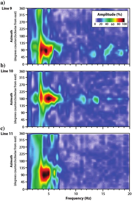
Passive MASW using 1D and 2D arrays                                                     EN65

                                                                                                                                                            sources that propagate along a linear and inline path similar to active   imaging, which stacks phase-velocity information at a given
                                                                                                                                                            seismic sources advancing along the geophone array. Although the          frequency increment (Park et al., 1998), frequency-azimuth plots
Downloaded 09/23/21 to 129.237.143.16. Redistribution subject to SEG license or copyright; see Terms of Use at http://library.seg.org/page/policies/terms

                                                                                                                                                            source itself cannot be controlled in terms of strength and distance,     are produced by stacking azimuth information at degree-angle in-
                                                                                                                                                            the direction of the source relative to the receiver lines can be esti-   crements for energy spanning a specified frequency range (Park
                                                                                                                                                            mated from a 2D grid array and incorporated into data processing.         et al., 2004). Recorded wavefronts are considered inline plane-wave
                                                                                                                                                            However, it may not always be feasible to deploy a 2D array that          propagation rather than spherical wave propagation because they
                                                                                                                                                            covers a test site in its entirety due to the size of a survey area or    originate from distances two times greater than the radius of the
                                                                                                                                                            limited equipment allowances. Instead, it has proven most effective       recording 2D array (Park, 2008).
                                                                                                                                                            to deploy a single 2D array at a fixed location central to multiple 1D       Given a 2D array, incoming surface-wave energy, E2D ðω; c; θÞ, is
                                                                                                                                                            receiver spreads with a size defined by the sensitivity to the longest    dependent on three parameters including frequency ω, scanning
                                                                                                                                                            wavelength expected. Such an approach can minimize field labor,           phase velocity c, and azimuth θ. This energy is estimated using
                                                                                                                                                            time, and data processing and contribute to using selective, higher       equation 1 from Park et al. (2004), where a phase shift φi is
                                                                                                                                                            quality data and thus final results.                                      applied to the Fourier transform Ri ðωÞ of ith trace along the x- and
                                                                                                                                                               The 1D–2D passive MASW method can be summarized in five                y-axes of the 2D array,
                                                                                                                                                            steps: (1) Collect passive seismic data simultaneously using one or
                                                                                                                                                            more 1D and a 2D receiver arrays, (2) select an optimal source rec-                         X               X            
                                                                                                                                                            ord using dispersion-curve images from 1D receiver spreads and                               NX             NY           
                                                                                                                                                                                                                                                        
                                                                                                                                                                                                                                         E2D ðω; c; θÞ ¼     jφ
                                                                                                                                                                                                                                                             e Rix ðωÞ þ
                                                                                                                                                                                                                                                                 ix         e Riy ðωÞ:
                                                                                                                                                                                                                                                                             jφ iy                     (1)
                                                                                                                                                            frequency versus azimuth angle images (i.e., frequency-azimuth
                                                                                                                                                                                                                                                            ix¼1                iy¼1
                                                                                                                                                            plots) from the 2D array, (3) estimate shorter optimal spread size
                                                                                                                                                            that meets desired project specifications (e.g., preserving lowest
                                                                                                                                                            frequencies for maximum depth analysis) and extract as many pos-          Energy is the absolute value of the summed NX and NY phase-
                                                                                                                                                            sible short-spread records with spread midstations that simulate          shifted traces. The estimated energy peaks are projected into
                                                                                                                                                            roll-along data acquisition, (4) create dispersion-curve images from      frequency-azimuth (ω-θ) space using the grid receiver coordinate
                                                                                                                                                            each roll-along spread segment and pick dispersion curves, and            system configured into 2D concentric square arrays using GPS-as-
                                                                                                                                                            (5) invert those picked curves for 1D V S sections that are combined      signed positions during acquisition (Figure 1). By performing these
                                                           DOI:10.1190/geo2020-0104.1

                                                                                                                                                            into quasi-2D V S sections (henceforth referred to as MASW V S            steps, linear trends will be mapped on frequency-azimuth plots
                                                                                                                                                            sections). Details pertaining to these steps are discussed in a later     (Figure 2) with respect to the frequency and azimuth (Park et al.,
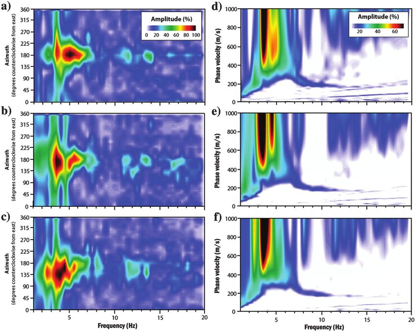
                                                                                                                                                            section. With the exception of steps 2 and 3, this procedure mimics       2008). The azimuth angle is measured in degrees counterclockwise
                                                                                                                                                            the active MASW method described earlier (Park et al., 1998; Miller       from east (0°) such that surface waves propagating from east to west
                                                                                                                                                            et al., 1999; Xia et al., 1999).                                          will plot across 180° (Figure 2a) and surface waves propagating
                                                                                                                                                               Great emphasis is given to source record selection, which is one       from west to east will plot along 0° (Figure 2b). Therefore, trends
                                                                                                                                                            of the core differences between the passive and active methods de-        illustrate the incoming direction or angle at which seismic energy
                                                                                                                                                            scribed here. Although many ambient noise methods combine all             was recorded traveling through the 2D grid array.
                                                                                                                                                            three components of the seismic wave, this method only considered
                                                                                                                                                            the vertical component for Rayleigh-wave velocity analysis.
                                                                                                                                                            Although the success of all dispersion-curve imaging and interpre-
                                                                                                                                                            tation is largely dependent on source signal quality, this specific
                                                                                                                                                            passive method relies on inline, low-frequency surface-wave signals
                                                                                                                                                            from sources at least 1–2 km from the receiver spread. These signals
                                                                                                                                                            are susceptible to varying degrees of overestimations, where un-
                                                                                                                                                            wanted, dominating offline ambient noise is recorded in the data.
                                                                                                                                                            For the purpose of this work, an ideal source signal has a coherent
                                                                                                                                                            seismic energy spectrum from 4 to 20 Hz that is concentrated within
                                                                                                                                                            a single azimuth angle coinciding with the orientation of the fixed
                                                                                                                                                            linear array. Details pertaining to azimuth-frequency imaging and
                                                                                                                                                            dispersion-curve processing are described in the following subsec-
                                                                                                                                                            tions using passive data from a well-documented test site in south-
                                                                                                                                                            central Kansas, USA.

                                                                                                                                                            Source record detection
                                                                                                                                                               The surface-wave azimuth image is generated using a 2D receiver
                                                                                                                                                            grid composed of four nested square arrays with 131 vertical geo-
                                                                                                                                                            phones at 5 m receiver spacing (Figure 1); the symmetric square
                                                                                                                                                            shape is used instead of a circle, triangle, or cross for positioning
                                                                                                                                                            convenience during survey deployment. The 2D array also limits
                                                                                                                                                            azimuth bias of the recorded signal by eliminating multidirectional
                                                                                                                                                            source environments from 1D array processing and to help identify         Figure 1. Four nested square arrays were deployed using 131 ver-
                                                                                                                                                            source records with single sources from a preferred incoming              tical geophones at 5 m spacing to construct the 2D grid to analyze
                                                                                                                                                            direction (Park and Miller, 2008). Similar to the dispersion-curve        source azimuth information.
Passive multichannel analysis of surface waves using 1D and 2D receiver arrays
EN66                                                             Morton et al.

                                                                                                                                                               For a given frequency, multiple energy peaks may exist at different    of surface-wave trends. For example, on a frequency-azimuth plot
                                                                                                                                                            phase velocities and azimuths if multiple surface-wave modes and en-      there may be high-amplitude energy imaged below 5 Hz, which
Downloaded 09/23/21 to 129.237.143.16. Redistribution subject to SEG license or copyright; see Terms of Use at http://library.seg.org/page/policies/terms

                                                                                                                                                            ergy sources are present. Dispersion-curve images are generated using     would imply the potential for imaging dominant longer wave-
                                                                                                                                                                       0
                                                                                                                                                            energy, E2D  ðω; cÞ, estimated with equation 2 (Park et al., 2004):       lengths. However, the corresponding dispersion-curve image may
                                                                                                                                                                                                                                      reveal that this high-amplitude energy is a combination of offline
                                                                                                                                                                                            X
                                                                                                                                                                                            Nθ                                        energy (i.e., seismic energy originating from sources propagating
                                                                                                                                                                              0 ðω; cÞ ¼
                                                                                                                                                                             E2D                  E2D ðω; c; θi Þ:            (2)     at an oblique angle relative to the linear array) and higher modes
                                                                                                                                                                                            i¼1                                       that are masking the fundamental-mode trend. It is preferred to se-
                                                                                                                                                                                                                                      lect dispersion-curve images whose low-frequency energy exhibits
                                                                                                                                                            All of the surface-wave energy is summed for N θ azimuths based on        well-defined wave separation to reduce mode misidentification and
                                                                                                                                                            the same scanning frequency and phase-velocity intervals from equa-       the need for slope filtering. The frequency-azimuth plot that meets
                                                                                                                                                            tion 1. These dispersion-curve images display constructively stacked      the described criteria is selected as the source record for generating
                                                                                                                                                            surface-wave dispersion trends from all sources recorded in the           dispersion-curve images along that survey line.
                                                                                                                                                            c-θ space. All of the data were processed using SurfSeis and                 Data are collected overnight for periods exceeding 12 h. These
                                                                                                                                                            KGS SeisUtilities, proprietary software packages developed by the         longer durations increase the opportunity to record seismic energy
                                                                                                                                                            Kansas Geological Survey.                                                 aligned with the fixed array’s orientation in the field. If a single source
                                                                                                                                                                                                                                      file does not contain sufficient S/N of low-frequency surface-wave am-
                                                                                                                                                            Source record selection                                                   plitudes, multiple source files with intermittent energy that otherwise
                                                                                                                                                                                                                                      meet the criteria for these source image files can be stacked to increase
                                                                                                                                                               For this method, it is critical that an adequate source record
                                                                                                                                                                                                                                      the S/N. It is important to note that only the dispersion-curve images
                                                                                                                                                            (i.e., frequency-azimuth plot) is selected to produce a coherent
                                                                                                                                                                                                                                      are stacked, not the raw seismic records. Caution should be taken when
                                                                                                                                                            dispersion-curve trend. An adequate source record includes linear
                                                                                                                                                                                                                                      stacking multiple frequency-azimuth plots to limit the variability of
                                                                                                                                                            frequency amplitude information that spans the desired frequency
                                                                                                                                                                                                                                      incoming energy and reduce aliasing. Then, spread tests are performed
                                                                                                                                                            range (e.g., 1–20 Hz) and is limited to a narrow range of angles
                                                                                                                                                                                                                                      to determine the shortest spread length that will yield the highest pos-
                                                                                                                                                            relative to the orientation of the 1D receiver spread (Figure 3a).
                                                                                                                                                                                                                                      sible lateral resolution without adversely affecting the fundamental-
                                                           DOI:10.1190/geo2020-0104.1

                                                                                                                                                            Source records that do not meet these guidelines have no dominant
                                                                                                                                                                                                                                      mode signature.
                                                                                                                                                            azimuth, and the frequency-azimuth plots appear as amplitude
                                                                                                                                                            anomalies focused in small or discontinuous frequency bands at
                                                                                                                                                            various angles (Figure 3b). On the frequency-azimuth plots (Fig-                            FIELD TEST EXAMPLES
                                                                                                                                                            ure 3), fundamental-mode energy cannot be differentiated from
                                                                                                                                                            higher modes or other noise energy. Therefore, corresponding                At a test site in southcentral Kansas (Figure 4), surface-wave data
                                                                                                                                                            dispersion-curve images are generated to assess the overall quality       were acquired to monitor changes in rock competency between the

                                                                                                                                                            Figure 2. Frequency-azimuth plots where (a) surface waves propa-          Figure 3. Examples of frequency-azimuth plots with (a) high-qual-
                                                                                                                                                            gating west to east are plotted across 180° and (b) surface waves         ity linear signals from record 3480 and (b) poor-quality multidirec-
                                                                                                                                                            propagating east to west are plotted across 0°.                           tional signals from record 3455.
Passive multichannel analysis of surface waves using 1D and 2D receiver arrays
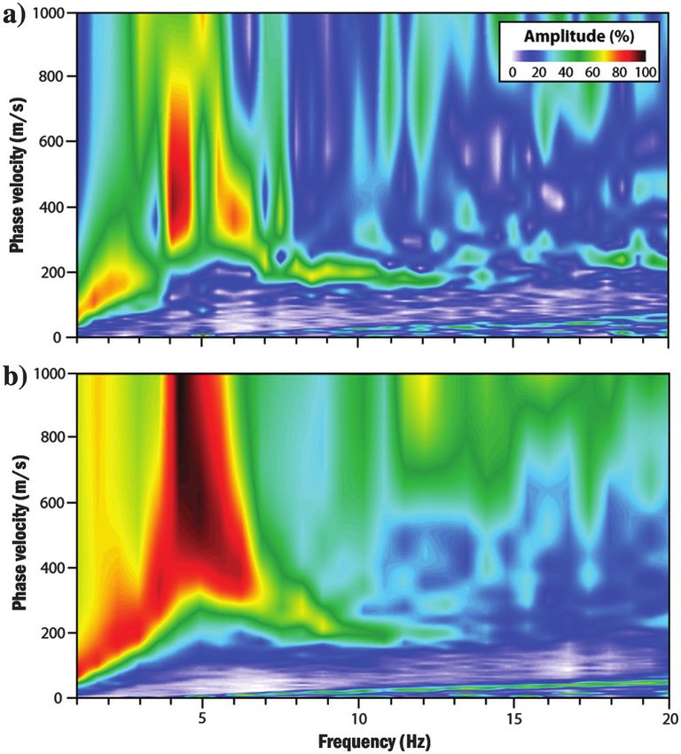
Passive MASW using 1D and 2D arrays                                                         EN67

                                                                                                                                                            Ninnescah Shale bedrock surface (approximately 21 m below ground            Active versus passive source data comparison
                                                                                                                                                            surface [BGS]) and basal contact of the Wellington Formation
                                                                                                                                                                                                                                           In 2008, an active seismic investigation of the Hutchinson Salt
Downloaded 09/23/21 to 129.237.143.16. Redistribution subject to SEG license or copyright; see Terms of Use at http://library.seg.org/page/policies/terms

                                                                                                                                                            (approximately 250 m BGS) in relation to the presence of known
                                                                                                                                                                                                                                        Member was performed using S-wave seismic reflection and conven-
                                                                                                                                                            dissolution-mined voids in the Hutchinson Salt Member of the Wel-
                                                                                                                                                            lington Formation (Walters, 1978; Ivanov et al., 2013; Morton et al.,       tional MASW data acquisition (Figure 4) to determine whether known
                                                                                                                                                                                                                                        dissolution-mined voids below wells and the associated in situ stress
                                                                                                                                                            2020). These approximately 30 m diameter dissolution-mined voids
                                                                                                                                                                                                                                        conditions could be detected noninvasively (Miller et al., 2009; Sloan
                                                                                                                                                            are referred to as salt jugs for their jug-like shape. Dissolution-mining
                                                                                                                                                                                                                                        et al., 2009). However, 7.8 Hz was the lowest frequency (f = v/λ)
                                                                                                                                                            operations using methods (e.g., single-well, multiwell, room-and-pil-
                                                                                                                                                                                                                                        achieved with the active MASW method on line 1 (Figure 5a). The
                                                                                                                                                            lar) susceptible to long-term void stability problems were common
                                                                                                                                                                                                                                        minimum and maximum depths of investigation can be estimated
                                                                                                                                                            throughout the late 19th and early 20th centuries. During that time,
                                                                                                                                                                                                                                        from these data sets because the approximate depth of investigation
                                                                                                                                                            these operations were much less regulated and lacked the engineering
                                                                                                                                                                                                                                        for Rayleigh waves is equal to its wavelength (Richart et al., 1970) and
                                                                                                                                                            design that is common in today’s practices and necessary to minimize
                                                                                                                                                                                                                                        the calculated depth of inverted S-wave velocities is half the wave-
                                                                                                                                                            void roof degradation and failure. Many well sites in this area remain
                                                                                                                                                                                                                                        length (Rix and Leipski, 1991). Therefore, the longest available wave-
                                                                                                                                                            susceptible to the vertical migration of these legacy voids and poten-
                                                                                                                                                                                                                                        length was only approximately 28 m (λmax ¼ 217∕7.8 ¼ 27.8 m),
                                                                                                                                                            tial ground failure (Walters, 1978).
                                                                                                                                                                                                                                        yielding a maximum depth of investigation of approximately 14 m
                                                                                                                                                               Because V S is directly related to the shear modulus, or stiffness,
                                                                                                                                                                                                                                        (zmax ¼ 27.8∕2 ¼ 13.9 m) and not penetrating the entire 21 m allu-
                                                                                                                                                            MASW V S sections from inverted surface-wave energy provide a
                                                                                                                                                                                                                                        vial interval. Survey parameters for the active MASW survey included
                                                                                                                                                            measure of material strength. Therefore, anomalous areas of de-
                                                                                                                                                                                                                                        (144) 4.5 Hz vertical geophones deployed at 1.8 m (4 ft) intervals, a
                                                                                                                                                            creased or increased V S correspond to areas of decreased stiffness
                                                                                                                                                                                                                                        6 m active-source offset, and a 42.67 m (140 ft) subspread extracted
                                                                                                                                                            (weakening) or increased stiffness (stress build up). With time-lapse
                                                                                                                                                                                                                                        from the fixed receiver spread (Table 1). Although some lower
                                                                                                                                                            surface-wave analysis, successful detection of these temporal veloc-
                                                                                                                                                                                                                                        frequencies were observed, the signal was attenuated between 5.5
                                                                                                                                                            ity variations and associated failure potential or evidence of
                                                                                                                                                                                                                                        and 7.0 Hz, limiting fundamental-mode interpretation within this
                                                                                                                                                            previous failure conditions provide early warnings that can allow
                                                                                                                                                                                                                                        frequency range (Figure 5a). Therefore, the 1D–2D passive MASW
                                                                                                                                                            action to minimize the impacts to infrastructure prior to sinkhole
                                                                                                                                                                                                                                        method was developed to instead use nearby passing trains (1–2 km
                                                           DOI:10.1190/geo2020-0104.1

                                                                                                                                                            development (Morton et al., 2020). In addition, estimates of depth
                                                                                                                                                                                                                                        away) as sources for lower frequency energy.
                                                                                                                                                            below the ground surface to halt the vertical migration of a void due
                                                                                                                                                                                                                                           In 2017, a new MASW survey was designed to acquire passive
                                                                                                                                                            to sufficient bulking can allow estimates of future ground stability.
                                                                                                                                                                                                                                        seismic data along the same spatial location of the 2008 active
                                                                                                                                                               Borehole logs report an average 21 m of alluvial materials and
                                                                                                                                                            Pliocene-Pleistocene Equus beds at the surface above the bedrock,
                                                                                                                                                            which is the Ninnescah Shale (Watney et al., 2003). The top of the
                                                                                                                                                            Hutchinson Salt Member varies from 60 to 80 m depth; therefore,
                                                                                                                                                            the depth of interest for this investigation is between 60 and 80 m.

                                                                                                                                                            Figure 4. Field test site in southcentral Kansas where linear receiver      Figure 5. Dispersion-curve images from (a) the 2008 active survey
                                                                                                                                                            spreads were deployed for active and passive seismic data acquis-           along line 1 and (b) 2017 passive survey along line 4. The curve
                                                                                                                                                            ition. The 2008 active MASW study included line 1 and the 2017              with the white squares represents picked active data set from 7.8 to
                                                                                                                                                            passive MASW study included lines 4, 9, 10, and 11. The location            39.4 Hz though data shown only to 20 Hz; the curve with the white
                                                                                                                                                            of the 2D grid used for passive acquisition is illustrated as four con-     circles represents picked passive data set from 4.5 to 20.0 Hz for
                                                                                                                                                            centric squares.                                                            brevity.
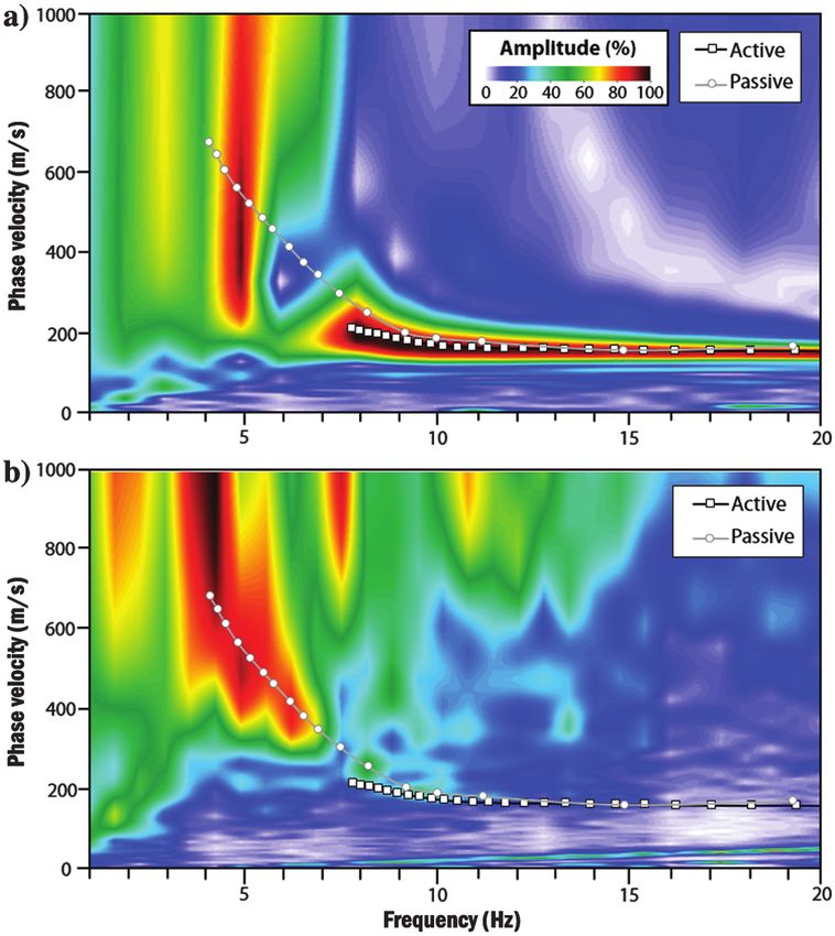
Passive multichannel analysis of surface waves using 1D and 2D receiver arrays
EN68                                                              Morton et al.

                                                                                                                                                            MASW data set (Figure 4). Line 4 was deployed with a 180° survey           pretation of dispersion curves from the 2008 active MASW data
                                                                                                                                                            line orientation relative to the east (Figure 1) and passive source en-    set was limited to frequencies >7 Hz (Figure 5a). The minimum
Downloaded 09/23/21 to 129.237.143.16. Redistribution subject to SEG license or copyright; see Terms of Use at http://library.seg.org/page/policies/terms

                                                                                                                                                            ergy generated by trains yielded high S/N, coherent fundamental-           and maximum wavelengths recorded were approximately 4 m
                                                                                                                                                            mode dispersion energy from 4.5 to 20.0 Hz (Figure 5b). Passive sur-       (λmin ¼ 156∕39.4 ¼ 3.8 m) and 28 m (λmax ¼ 217∕7.8 ¼ 27.8 m)
                                                                                                                                                            vey parameters for line 4 included (168) 4.5 Hz vertical geophones         (Figure 5a), which correspond to 2–14 m inverted depths
                                                                                                                                                            deployed at 3 m intervals and an optimal 84 m subspread extracted          (zmin ¼ 3.8∕2 ¼ 1.9 m; zmax ¼ 27.8∕2 ¼ 13.9 m). The 1D–2D
                                                                                                                                                            from a fixed 1D receiver spread (Table 1). To determine the direction      passive MASW method achieved greater penetration depths com-
                                                                                                                                                            of passive source energy relative to the linear receiver spread, a 2D      pared with the active method (Figure 6b). The velocity structure
                                                                                                                                                            square grid array was also deployed, which consisted of four concen-       in Figure 6b is consistent with alluvial materials sampled from 0
                                                                                                                                                            tric squares of 4.5 Hz vertical geophones spaced at 5 m intervals.         to 21 m, the (weaker) Ninnescah Shale and the (firmer) Wellington
                                                                                                                                                               Fundamental-mode trends from the active (Figure 5a) and passive         Formation from 21 to 80 m, and the Hutchinson Salt Member below
                                                                                                                                                            (Figure 5b) surveys are superimposed on dispersion-curve images in         80 m. The minimum and maximum wavelengths recorded were ap-
                                                                                                                                                            which both images have similar trends at frequencies greater than          proximately 9 m (λmin ¼ 172∕19.3 ¼ 8.9 m) and 167 m (λmax ¼
                                                                                                                                                            9 Hz. Phase velocity did vary by an average of 11% between 7               684.6∕4.1 ¼ 166.9 m) (Figure 5b), which correspond to 4.5–83.5 m
                                                                                                                                                            and 10 Hz due to differences in dispersion-curve image resolution          inverted depths (zmin ¼ 8.9∕2 ¼ 4.45 m; zmax ¼ 166.9∕2 ¼ 83.45 m).
                                                                                                                                                            and receiver spread size between the active and passive data               Compared to the MASW V S section from active data, the average
                                                                                                                                                            sets. The resulting MASW V S sections for lines 1 and 4 from the           velocity of the uppermost layer was within 10% of that estimated
                                                                                                                                                            active and passive studies, respectively, are shown in Figure 6. Inter-    in the passive MASW V S section. Based on this work, other recent
                                                                                                                                                                                                                                       passive MASW surveys conducted at this test site (Ivanov et al., 2013;
                                                                                                                                                                                                                                       Morton et al., 2020), and the consistency between the velocity struc-
                                                                                                                                                            Table 1. Active and passive survey geometry.                               ture and known material characteristics, this 1D–2D passive MASW
                                                                                                                                                                                                                                       method successfully imaged an average 77 m depth of investigation
                                                                                                                                                                                                                                       using passing trains as a passive seismic source. This average depth to
                                                                                                                                                                                          Active survey            Passive survey
                                                                                                                                                            Parameter                        (line 1)                 (line 4)         the half-space layer is within range of the Wellington Shale-Hutchin-
                                                           DOI:10.1190/geo2020-0104.1

                                                                                                                                                                                                                                       son Salt Member boundary at a depth of 80 m that the active survey
                                                                                                                                                            Receiver spacing                 1.8 m                      3m             could not achieve.
                                                                                                                                                            Source type                    Weight drop                 Trains
                                                                                                                                                            Source offset                     6m                       >1 km           180°, 90°, and 74° survey line orientations
                                                                                                                                                            Optimal spread size             42.67 m                    84 m               The 2D grid consists of four concentric squares that are deployed
                                                                                                                                                                                                                                       using (131) 4.5 Hz vertical geophones at 5 m spacing. In addition to
                                                                                                                                                                                                                                       this 2D grid, several fixed linear arrays using 4.5 Hz vertical geo-
                                                                                                                                                                                                                                       phones at 3 m spacing are also deployed to monitor stress condi-
                                                                                                                                                                                                                                       tions surrounding other wells in this field area; total spread lengths
                                                                                                                                                                                                                                       vary from 200 to 250 m (Figure 4). These linear arrays are later
                                                                                                                                                                                                                                       decimated into shorter rolling spreads (e.g., 70–120 m) for
                                                                                                                                                                                                                                       dispersion-curve processing.
                                                                                                                                                                                                                                          Energy from passing trains (i.e., 1–2 km away) has turned out to
                                                                                                                                                                                                                                       be the preferred ambient noise source at this site used to obtain long
                                                                                                                                                                                                                                       enough wavelengths to sufficiently image depths greater than 30 m
                                                                                                                                                                                                                                       rather than residential vehicle traffic or other sources. The arrival
                                                                                                                                                                                                                                       and incoming direction of each passing train were verified by
                                                                                                                                                                                                                                       the seismic survey operator based on calibrated observations such
                                                                                                                                                                                                                                       as train noise (e.g., train whistle or horn) and the seismograph’s
                                                                                                                                                                                                                                       noise floor during overnight acquisition of seismic records. These
                                                                                                                                                                                                                                       calibrated observations were initially provided by field personnel to
                                                                                                                                                                                                                                       allow the survey operator to develop a qualitative method to esti-
                                                                                                                                                                                                                                       mate the incoming train distance. In the current approach, the sur-
                                                                                                                                                                                                                                       vey operator takes similar observations into consideration during
                                                                                                                                                                                                                                       source record selection. Passive seismic data (Figure 7) are col-
                                                                                                                                                                                                                                       lected nearly continuously in consecutive 30 s records (2 ms sam-
                                                                                                                                                                                                                                       pling rate) throughout the night from the 1D linear receiver spreads
                                                                                                                                                                                                                                       and 2D grid. Although freight or cargo train energy is considered
                                                                                                                                                                                                                                       optimal for surface-wave generation, all local sources are consid-
                                                                                                                                                                                                                                       ered during data processing if their wave-propagation direction
                                                                                                                                                            Figure 6. The MASW V S section with true velocity values from              is aligned or closely aligned with the linear arrays. Data from
                                                                                                                                                            lines 1 and 4 data sets; the geographic location of line 1 is the same     the 2D grid are used as a quality control measure of this incoming
                                                                                                                                                            as line 4. (a) The 2008 active MASW survey result had a limited
                                                                                                                                                            depth of investigation compared to (b) the 2017 1D–2D passive              wave energy and wave azimuth. Seismic data records with energy
                                                                                                                                                            MASW survey result.                                                        azimuths aligned with one or more of the fixed linear arrays are
Passive multichannel analysis of surface waves using 1D and 2D receiver arrays
Passive MASW using 1D and 2D arrays                                                        EN69

                                                                                                                                                            preferred during selection of a source record for processing that              Source selection was also performed for lines 9 and 11, which
                                                                                                                                                            linear array.                                                               were deployed to monitor other areas known to contain dissolution
Downloaded 09/23/21 to 129.237.143.16. Redistribution subject to SEG license or copyright; see Terms of Use at http://library.seg.org/page/policies/terms

                                                                                                                                                               Because the wavelengths required to image the entire shale cap-          voids. Based on the survey map shown in Figure 4, the orientation
                                                                                                                                                            rock corresponded to 40–80 m depth or approximately 4.5–7.0 Hz,             of line 9 was 86° and the orientation of line 11 was 74°. High-
                                                                                                                                                            it was critical that high-amplitude coherent energy within this fre-        amplitude energy is observed from approximately 3.5 to 6.5 Hz
                                                                                                                                                            quency range was recorded to optimize the calculation of dispersion         in each of the three optimal source records selected for lines 9–11
                                                                                                                                                            curves and the interpretation of the image. Therefore, source records       (Figure 9). For line 9, the optimal source record 2746 (Figure 9a)
                                                                                                                                                            with dominant, inline, or parallel-wave energy along azimuths cor-          had an 88° azimuth, resulting in a 2° differential between the source
                                                                                                                                                            responding to each line were selected for processing. Frequency-            azimuth and array orientation. Previously discussed source record
                                                                                                                                                            azimuth plots shown in Figure 8a–8c provide examples of potential           1345 (Figure 9b) was selected for line 10 with a 181° azimuth and 1°
                                                                                                                                                            source records for line 10 with varying signal quality and content.         differential. Source record selection proved more challenging for
                                                                                                                                                            Figure 8a was selected for processing because the highest-ampli-            line 11, but source record 1092 with a 96° azimuth (Figure 9c)
                                                                                                                                                            tude energies are observed with 180° azimuth
                                                                                                                                                            compared with Figure 8b, which shows recorded
                                                                                                                                                            omnidirectional source signal (i.e., 0°–360°) be-
                                                                                                                                                            tween 2.5 and 5.0 Hz. Because Figure 8c displays
                                                                                                                                                            the recorded source signal at the incorrect azimuth
                                                                                                                                                            angle (150°), it was also not selected to avoid in-
                                                                                                                                                            terference from offline sources.
                                                                                                                                                               Dispersion-curve images were also generated
                                                                                                                                                            for each frequency-azimuth plot (Figure 8d–8f);
                                                                                                                                                            these provide additional insight about the corre-
                                                                                                                                                            sponding dispersion characteristics of the recorded
                                                                                                                                                            source signal. They are used primarily to deter-
                                                           DOI:10.1190/geo2020-0104.1

                                                                                                                                                            mine whether high-amplitude energy corresponds
                                                                                                                                                            to the fundamental mode and not numerical arti-
                                                                                                                                                            facts such as spectral leakage (Ivanov et al., 2015).
                                                                                                                                                            Because dispersion-curve images are generated
                                                                                                                                                                                                                    Figure 7. Example shot record 2089 displaying signal from an approaching train.
                                                                                                                                                            using the 2D square grid array, they are used to
                                                                                                                                                            guide source selection only, not inversion.
                                                                                                                                                               For these line 10 source records (Figure 8),
                                                                                                                                                            dispersion characteristics exhibit comparable fre-
                                                                                                                                                            quency content and phase velocity ranges. Below
                                                                                                                                                            3.5 Hz in Figure 8d, the offline source signal is at
                                                                                                                                                            a minimum with relatively coherent fundamen-
                                                                                                                                                            tal-mode energy until 17 Hz despite mode energy
                                                                                                                                                            becoming increasingly attenuated. In Figure 8e,
                                                                                                                                                            aliasing is more prevalent below 3.5 Hz and the
                                                                                                                                                            fundamental mode is less discernible between
                                                                                                                                                            3.5 and 5.0 Hz due to a potential high-velocity,
                                                                                                                                                            higher mode in the same frequency range. This
                                                                                                                                                            may be attributed to the omnidirectional source
                                                                                                                                                            energies observed in Figure 8b within the same
                                                                                                                                                            frequency range. The dispersion-curve image in
                                                                                                                                                            Figure 8f is generally consistent with Figure 8d
                                                                                                                                                            with strong energy at 3.5 Hz, but the signal is
                                                                                                                                                            slightly more attenuated between 3.5 and 7.0 Hz
                                                                                                                                                            in Figure 8f. It is expected that the phase-velocity
                                                                                                                                                            trend in Figure 8f will also deviate from the true
                                                                                                                                                            value due to its off-angle source azimuth (i.e.,
                                                                                                                                                            150°). Overall, these dispersion-curve images
                                                                                                                                                            provided additional quality control of the re-
                                                                                                                                                            corded source characteristics by revealing attenu-
                                                                                                                                                            ated signal and interference from possible higher
                                                                                                                                                            modes or oblique-angle sources. Based on its            Figure 8. Line 10 frequency-azimuth plot from (a) source record 1345, (b) source record
                                                                                                                                                            180° directionality (Figure 8a) and higher ampli-       1087, and (c) source record 1089. Each frequency-azimuth plot has a corresponding
                                                                                                                                                                                                                    dispersion-curve image representing all energy recorded with the full 2D receiver grid.
                                                                                                                                                            tude and uninterrupted fundamental-mode trend           These corresponding dispersion-curve images from (d) source record 1345, (e) source
                                                                                                                                                            (Figure 8d), source record 1345 was selected for        record 1087, and (f) source record 1089 are used to evaluate the quality of the recorded
                                                                                                                                                            processing line 10.                                     source signal and guide source record selection.
Passive multichannel analysis of surface waves using 1D and 2D receiver arrays
EN70                                                                 Morton et al.

                                                                                                                                                            was chosen based on the high-amplitude, continuous energy                     Subsequently, phase velocities were slightly lower in Figure 10c
                                                                                                                                                            recorded from approximately 3.5 to 5.0 Hz. This 22° differential              compared with phase velocities observed on lines 9 and 10 (Fig-
Downloaded 09/23/21 to 129.237.143.16. Redistribution subject to SEG license or copyright; see Terms of Use at http://library.seg.org/page/policies/terms

                                                                                                                                                            between the line orientation (74°) and source azimuth (96°) is easily         ure 10a and 10b, respectively). The fundamental mode did vary
                                                                                                                                                            accounted for following the scale property (Socco and Boiero,                 across line 10 with western stations having slightly higher phase
                                                                                                                                                            2008) after dispersion-curve inversion using (Park et al., 2004)              velocities than eastern stations. Maximum wavelengths recorded at
                                                                                                                                                                                                                                          western stations were approximately 132 m (λmax ¼ 627∕4.7 ¼
                                                                                                                                                                                  V S;true ¼ V S;app  cos θ:                     (3)     132 m) and 201 m (λmax ¼ 724∕3.6 ¼ 201 m), which correspond
                                                                                                                                                                                                                                          to maximum depths varying from 66 to 100.5 m (Figure 11b) from
                                                                                                                                                                                                                                          west to east (zmax ¼ 132∕2 ¼ 66 m; zmax ¼ 201∕2 ¼ 100.5 m).
                                                                                                                                                            After dispersion-curve inversion, apparent velocities (V S;app ) are
                                                                                                                                                                                                                                          Nonetheless, picked dispersion curves were inverted to create
                                                                                                                                                            converted to true velocities (V S;true ), where θ is the degree difference
                                                                                                                                                            between the array and source azimuths.
                                                                                                                                                               After source records were selected for each line, optimal spread
                                                                                                                                                            sizes were extracted from the fixed receiver spreads (Table 2). In gen-       Table 2. Survey geometry for linear receiver spreads during
                                                                                                                                                            eral, high-amplitude fundamental-mode energy was observed from                passive acquisition.
                                                                                                                                                            approximately 4.0 to 7.0 Hz for each line (Figure 10) with signal
                                                                                                                                                            attenuating gradually at higher frequencies. Dispersion curves from           Line    Line azimuth      Source azimuth      Optimal spread size
                                                                                                                                                            line 9 (Figure 10a) and line 10 (Figure 10b) exhibited a dominant
                                                                                                                                                            fundamental mode with minimal interference from higher modes.                 9             86°               88°                  84 m
                                                                                                                                                            However, higher modes were more prevalent on line 11 (Figure 10c,             10           181°              180°                  84 m
                                                                                                                                                            e.g., approximately 1000 m/s at 4 Hz and 800 m/s at 7.0 Hz), which            11            74°               96°                  87 m
                                                                                                                                                            reduced coherency of the fundamental mode above 7.0 Hz.
                                                           DOI:10.1190/geo2020-0104.1

                                                                                                                                                            Figure 9. Source records selected for (a) line 9 with 88° source azi-
                                                                                                                                                            muth, (b) line 10 with 181° source azimuth, and (c) line 11 with 92°          Figure 10. Representative dispersion-curve images from (a) line 9,
                                                                                                                                                            source azimuth.                                                               (b) line 10, and (c) line 11.
Passive multichannel analysis of surface waves using 1D and 2D receiver arrays
Passive MASW using 1D and 2D arrays                                                     EN71

                                                                                                                                                            MASW V S sections for each line (Figure 11); equation 3 was used to       the project while eliminating labor costs associated with operating
                                                                                                                                                            account for apparent velocity. Lines 9 and 10 had greater depths of       an active seismic source. By removing the active source from the
Downloaded 09/23/21 to 129.237.143.16. Redistribution subject to SEG license or copyright; see Terms of Use at http://library.seg.org/page/policies/terms

                                                                                                                                                            investigation than line 11, but the observed bulk-velocity trends were    survey, noise associated with running the active seismic source and
                                                                                                                                                            generally consistent with documented geologic materials in this area      potential damage or disturbance to the survey area are no longer
                                                                                                                                                            (Miller et al., 2009). With respect to velocity variations, no anoma-     factors to consider when working in either urban, rural, or agricul-
                                                                                                                                                            lously high- or low-velocity features were interpreted on line 9 based    tural environments.
                                                                                                                                                            on the uniformity observed across the MASW V S section (Fig-                 Certain considerations need to be taken into account during sur-
                                                                                                                                                            ure 11a). The eastern portion of line 10 (below stations 1040–1055)       vey design and data processing when using the 1D–2D passive
                                                                                                                                                            was noted for reduced V S below 60 m relative to the western portion      MASW method. As proven at this test site, it is also advisable that
                                                                                                                                                            of the MASW V S section (Figure 11b). Finally, the average velocity       data acquisition extend across several hours to increase the oppor-
                                                                                                                                                            of the 25–65 m depth interval was lower on line 11 (Figure 11c) than      tunity for successfully recording adequate source energy because
                                                                                                                                                            lines 9 and 10. Based on these surveys, the 1D–2D passive MASW            the source signal quality and azimuth cannot be controlled by the
                                                                                                                                                            method has successfully produced MASW V S sections with depths            operator. If a source signal with an azimuth that corresponds to the
                                                                                                                                                            greater than 60 m; maximum depth of investigation exceeded 75 m           linear array is not recorded, the resulting apparent velocity values
                                                                                                                                                            on line 9 and parts of line 10.                                           can be adjusted to their true velocity value. From this study at this
                                                                                                                                                                                                                                      site, the best fundamental-mode dispersion trends were obtained
                                                                                                                                                                                      DISCUSSION                                      when the recorded source-to-line azimuth was within 18°, or the
                                                                                                                                                                                                                                      apparent velocity is within 5% of the true velocity. Above 5%, in-
                                                                                                                                                               Some multicomponent processing schemes assume that the am-             terference from offline sources degraded the coherency of the
                                                                                                                                                            bient noise signal is evenly distributed across all azimuths (Hayashi
                                                                                                                                                                                                                                      fundamental-mode trend.
                                                                                                                                                            et al., 2015), whereas some suggest that the source distribution
                                                                                                                                                                                                                                         Higher-mode interference and lack of fundamental-mode coher-
                                                                                                                                                            across a 90° angle is sufficient (Asten and Hayashi, 2018). The
                                                                                                                                                                                                                                      ency are two of the more common pitfalls encountered with
                                                                                                                                                            1D–2D passive MASW technique presented here uses a single dom-
                                                                                                                                                            inant source direction to optimize signal processing. This approach
                                                                                                                                                            can be used in areas where multiple, dominant inline sources are
                                                           DOI:10.1190/geo2020-0104.1

                                                                                                                                                            readily available unlike some of the other passive methods (e.g.,
                                                                                                                                                            SPAC); in this case, each of the trains can be treated as an individual
                                                                                                                                                            source. In addition, this unidirectional technique limits signal inter-
                                                                                                                                                            ference because the frequency-azimuth plot selected for processing
                                                                                                                                                            exhibits incoming source energy that aligns with the seismic
                                                                                                                                                            array. This focusing increases the S/N and overall quality of the
                                                                                                                                                            resulting calculations without the risk of near-field effects that
                                                                                                                                                            can occur with seismic interferometry (Cheng et al., 2015; Zhang
                                                                                                                                                            et al., 2019). Dispersion curves generated based on their azimuth
                                                                                                                                                            angle allowed apparent velocity to be corrected to true velocity val-
                                                                                                                                                            ues, minimizing errors in the final MASW V S sections. In addition,
                                                                                                                                                            a unique benefit of the 1D–2D passive MASW method is the ability
                                                                                                                                                            to measure anisotropy using perpendicular 1D arrays each with op-
                                                                                                                                                            timally aligned sources as demonstrated at this site by Morton
                                                                                                                                                            et al. (2020).
                                                                                                                                                               Key factors that contribute to successful passive processing in-
                                                                                                                                                            clude recording high S/N and broadband low-frequency content
                                                                                                                                                            (e.g., 1–20 Hz) of the seismic source signal. Ambient noise pro-
                                                                                                                                                            duced by trains 1–2 km away has been the best source of seismic
                                                                                                                                                            signal for this test site, and data acquisition has been customized to
                                                                                                                                                            allow for optimized processing. Compared with other passive seis-
                                                                                                                                                            mic techniques such as HVSR or SPAC, this passive MASW ap-
                                                                                                                                                            proach only uses a single 30 s record to produce a dispersion
                                                                                                                                                            image rather than a long continuous record (e.g., 30–60 min).
                                                                                                                                                            Dispersion-curve images from multiple 30 s source records may
                                                                                                                                                            be stacked if source records possess the same dominant source azi-
                                                                                                                                                            muth. This can improve the fundamental-mode dispersion trend co-
                                                                                                                                                            herency, but for this study, a single record has proven sufficient.
                                                                                                                                                            Although this may not be a direct advantage over other passive
                                                                                                                                                            methods at this test site because the demonstrated acquisition time
                                                                                                                                                            has been 10–12 h, the acquisition window can be minimized by
                                                                                                                                                            coordinating acquisition with train schedules. If multiple seismic
                                                                                                                                                            arrays with different orientations are required, these linear arrays
                                                                                                                                                            can be deployed in conjunction with the same 2D square grid array.        Figure 11. The MASW V S section with true velocity values from
                                                                                                                                                            Therefore, surveys of large areas can be designed to fit the needs of     (a) line 9, (b) line 10, and (c) line 11.
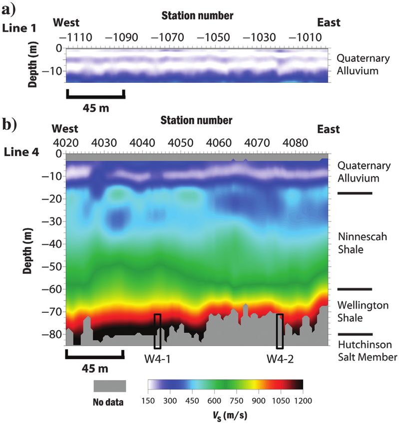
Passive multichannel analysis of surface waves using 1D and 2D receiver arrays
EN72                                                             Morton et al.

                                                                                                                                                            this passive MASW imaging method, both of which are strongly              are controlled by a multiplier. This multiplier helps to create a more
                                                                                                                                                            attributed to the quality of the recorded source signal. The near-sur-    continuous dispersion image as shown in Figure 12. Figure 12a
Downloaded 09/23/21 to 129.237.143.16. Redistribution subject to SEG license or copyright; see Terms of Use at http://library.seg.org/page/policies/terms

                                                                                                                                                            face environment is often riddled with local heterogeneities that         shows subrecord 13064 without window-selection processing, and
                                                                                                                                                            support the development of higher modes and restrict the imaging          Figure 12b illustrates how the surface-wave trend images greater
                                                                                                                                                            of longer fundamental-mode wavelengths with respect to surface-           continuity with window-selection processing. An awareness of the
                                                                                                                                                            wave sampling at depths greater than 30 m (O’Neill and Matsuoka,          fundamental-mode trend prior to attempting window-selection
                                                                                                                                                            2005). To better identify heterogeneities, Ivanov et al. (2008) rec-      processing is necessary due to the potential for overlapping higher
                                                                                                                                                            ommend decreasing the spread size to increase horizontal resolution       modes to interfere with the fundamental mode. This can lead
                                                                                                                                                            at the expense of limiting spread sensitivity to longer wavelengths       to mode misidentification and an inversion result that inaccurately
                                                                                                                                                            and consequently limiting the depth of investigation. The high-res-       represents the in situ geologic conditions.
                                                                                                                                                            olution linear radon transform (HRLRT) method (Luo et al., 2008a,            Dispersion-curve stitching is another tool for creating a continu-
                                                                                                                                                            2008b) has proven successful for isolating the higher and funda-          ous and coherent energy trend (KGS, 2017). For example, low-fre-
                                                                                                                                                            mental modes in these passive MASW data (Ivanov et al., 2017b)            quency signal from subrecord 13064 (Figure 13a) can be combined
                                                                                                                                                            and active seismic investigations (Ivanov et al., 2017a). If the          with higher frequency content from subrecord 13051 (Figure 13b)
                                                                                                                                                            HRLRT method is unable to discretize different dispersion trends          to produce an enhanced dispersion trend (Figure 13c). These lower
                                                                                                                                                            at low frequencies, the dispersion-curve frequency-wavenumber             and higher frequency dispersion-curve sections are stitched together
                                                                                                                                                            method (Park et al., 2002) can be used to filter higher mode energies
                                                                                                                                                            by designing a targeted filter zone to reduce unwanted passive
                                                                                                                                                            surface-wave energy. If performed successfully, higher modes are
                                                                                                                                                            reduced, allowing the fundamental-mode energy to dominate the
                                                                                                                                                            filtered frequency range.
                                                                                                                                                                Window-selection processing (KGS, 2017; Morton et al., 2019)
                                                                                                                                                            is another advanced imaging technique that can enhance the con-
                                                                                                                                                            tinuity of the dispersion trend. The algorithm divides the seismic
                                                                                                                                                            record into evenly timed sections, and then windows are selected
                                                           DOI:10.1190/geo2020-0104.1

                                                                                                                                                            based on a user-assigned root-mean-square criterion; these selected
                                                                                                                                                            time window(s) are used to generate dispersion-curve images. This
                                                                                                                                                            method is common in ambient noise processing such as HVSR
                                                                                                                                                            (Nakamura, 1989), in which the user chooses which signals qualify
                                                                                                                                                            for optimal processing. In theory, window-selection processing is
                                                                                                                                                            similar to automatic gain control in that the output amplitudes

                                                                                                                                                                                                                                      Figure 13. Example of stitched dispersion images in which (a) 1.0–
                                                                                                                                                                                                                                      7.0 Hz from subrecord 13064 are processed using the time-window
                                                                                                                                                                                                                                      splitting algorithm, (b) 7.0–20.0 Hz from subrecord 13051 are proc-
                                                                                                                                                                                                                                      essed with the conventional dispersion imaging algorithm, which are
                                                                                                                                                            Figure 12. Example dispersion curve from subrecord 13064 (a) be-          then (c) stitched together to form a combined dispersion-curve image.
                                                                                                                                                            fore and (b) after window-selection processing was applied on sub-        Dispersion information below 4.0 Hz is likely a numerical artifact
                                                                                                                                                            record 1069 during dispersion image generation.                           and is not considered for data processing.
Passive MASW using 1D and 2D arrays                                                           EN73

                                                                                                                                                            at a specific frequency value, allowing the user to use frequencies                           ACKNOWLEDGMENTS
                                                                                                                                                            obtained from more than one subrecord. Sections of dispersion im-
                                                                                                                                                                                                                                         The authors graciously thank the dedicated reviewers and editors
Downloaded 09/23/21 to 129.237.143.16. Redistribution subject to SEG license or copyright; see Terms of Use at http://library.seg.org/page/policies/terms

                                                                                                                                                            ages may be stitched together to also combine multiple imaging
                                                                                                                                                            techniques (e.g., the phase-shift method, HRLRT), different-sized         whose comments and suggestions greatly improved the quality of
                                                                                                                                                            receiver arrays, and source types to enhance the dispersion curve.        our paper. This work would not have been possible without the
                                                                                                                                                            Once stitched dispersion images are created, high-confidence trends       members of the Kansas Geological Survey Seismic Team who con-
                                                                                                                                                            can be picked, and these curves are used as input for 1D inversion        tributed to the development of this passive MASW method.
                                                                                                                                                            processing (Xia et al., 1999).
                                                                                                                                                               Given the nature of surface-wave propagation, the amount of                   DATA AND MATERIALS AVAILABILITY
                                                                                                                                                            averaging in the vertical direction used to produce the final MASW
                                                                                                                                                            V S section increases as the depth of investigation increases. For this      Data associated with this research are confidential and cannot be
                                                                                                                                                            reason, the deepest inverted layer (half-space layer) may not be part     released.
                                                                                                                                                            of the velocity interpretation. Therefore, interpretations of these
                                                                                                                                                            passive data results are performed based on the overall behavior of                                  REFERENCES
                                                                                                                                                            the measured area (Foti et al., 2014), such as changes in the bulk-
                                                                                                                                                                                                                                      Aki, K., 1957, Space and time spectra of stationary stochastic waves with
                                                                                                                                                            velocity structure, rather than fine details (Morton et al., 2020).         special reference of microtremors: Bulletin of the Earthquake Research
                                                                                                                                                            Shallow velocity inversions can also appear as artifacts of the lay-        Institute, 35, 415–456.
                                                                                                                                                            ered depth model, and are most often related to inversion instabil-       Akkaya, I., and A. Özvan, 2019, Site characterization in the Van settlement
                                                                                                                                                                                                                                        (Eastern Turkey) using surface waves and HVSR microtremor methods:
                                                                                                                                                            ities generally due to a lack of high-frequency dispersion-curve            Journal of Applied Geophysics, 160, 157–170, doi: 10.1016/j.jappgeo
                                                                                                                                                            information that corresponds to the shortest wavelengths associated         .2018.11.009.
                                                                                                                                                            with these depths; lack of sufficient data can be an issue for any        Asten, M., T. Dhu, and N. Lam, 2004, Optimised array design for micro-
                                                                                                                                                                                                                                        tremor array studies applied to site classification: Comparison of results
                                                                                                                                                            inversion scheme. These inversion features are verified through             with SCPT logs: 13th World Conference on Earthquake Engineering
                                                                                                                                                            careful analysis of the picked dispersion trends and experience with        Proceedings, 16.
                                                                                                                                                                                                                                      Asten, M. W., 2006, On bias and noise in passive seismic data from finite
                                                                                                                                                            the data set and processing procedures.                                     circular array data processing using SPAC methods: Geophysics, 71,
                                                                                                                                                                                                                                        no. 6, V153–V162, doi: 10.1190/1.2345054.
                                                           DOI:10.1190/geo2020-0104.1

                                                                                                                                                                                                                                      Asten, M. W., and K. Hayashi, 2018, Application of the spatial auto-corre-
                                                                                                                                                                                                                                        lation method for shear-wave velocity studies using ambient noise: Sur-
                                                                                                                                                                                     CONCLUSION                                         veys in Geophysics, 39, 633–659, doi: 10.1007/s10712-018-9474-2.
                                                                                                                                                                                                                                      Beroya, M. A. A., A. Aydin, R. Tiglao, and M. Lasala, 2009, Use of micro-
                                                                                                                                                               The presented 1D–2D passive MASW method has successfully                 tremor in liquefaction hazard mapping: Engineering Geology, 107, 140–
                                                                                                                                                                                                                                        153, doi: 10.1016/j.enggeo.2009.05.009.
                                                                                                                                                            imaged depths greater than 75 m in which the conventional active          Bodet, L., O. Abraham, and D. Clorennec, 2009, Near-offset effects on
                                                                                                                                                            MASW method was limited to 14 m at a test site in southcentral              Rayleigh-wave dispersion measurements: Physical modeling: Journal of
                                                                                                                                                            Kansas. This method has also proven advantageous because high-              Applied Geophysics, 68, 95–103, doi: 10.1016/j.jappgeo.2009.02.012.
                                                                                                                                                                                                                                      Bonnefoy-Claudet, S., C. Cornou, P.-Y. Bard, F. Cotton, P. Moczo, J.
                                                                                                                                                            amplitude surface-wave source information is easily recorded                Kristek, and D. Fäh, 2006, H/V ratio: A tool for site effects evaluation.
                                                                                                                                                            because high-energy sources (i.e., trains) are a part of the local ur-      Results from 1-D noise simulations: Geophysical Journal International,
                                                                                                                                                                                                                                        167, 827–837, doi: 10.1111/j.1365-246X.2006.03154.x.
                                                                                                                                                            ban environment. Train energy has proven to generate coherent             Capon, J., 1969, High-resolution frequency-wavenumber spectrum analysis:
                                                                                                                                                            dispersion curves at this site even though signal coherency can be          Proceedings of the IEEE, 57, 1408–1418, doi: 10.1109/PROC.1969.7278.
                                                                                                                                                            quite variable from record to record. Conventional mechanical seis-       Carniel, R., P. Malisan, F. Barazza, and S. Grimaz, 2008, Improvement of
                                                                                                                                                                                                                                        HVSR technique by wavelet analysis: Soil Dynamics and Earthquake
                                                                                                                                                            mic sources such as an accelerated weight drop or sledgehammer              Engineering, 28, 321–327, doi: 10.1016/j.soildyn.2007.06.006.
                                                                                                                                                            source were not necessary to augment for this work, reducing not          Chavéz-Garcia, F. J., M. Rodriguez, and W. R. Stephenson, 2006, Subsoil
                                                                                                                                                            only the labor costs but also the amount of equipment necessary to          structure using SPAC measurements along a line: Bulletin of the Seismo-
                                                                                                                                                                                                                                        logical Society of America, 96, 729–736.
                                                                                                                                                            be brought to the field site.                                             Cheng, F., J. Xia, Y. Luo, Z. Xu, L. Wang, C. Shen, R. Liu, Y. Pan, B. Mi,
                                                                                                                                                               Our unique combination of simultaneously using conventional              and Y. Hu, 2016, Multichannel analysis of passive surface waves based on
                                                                                                                                                                                                                                        crosscorrelations: Geophysics, 81, no. 5, EN57–EN66, doi: 10.1190/
                                                                                                                                                            linear array(s) and an additional 2D nested square grid allowed             geo2015-0505.1.
                                                                                                                                                            us to use existing source signals and achieve a greater depth of in-      Cheng, F., J. Xia, Z. Xu, Y. Hu, and B. Mi, 2017, Frequency-wavenumber
                                                                                                                                                            vestigation with minimal additional steps. The main contribution of         (FK)-based data selection in high-frequency passive surface wave survey:
                                                                                                                                                                                                                                        Surveys in Geophysics, 39, 661–682, doi: 10.1007/s10712-018-9473-3.
                                                                                                                                                            our efforts is the use of this additional 2D receiver grid as an analy-   Cheng, F., J. Xia, Y. Xu, Z. Xu, and Y. Pan, 2015, A new passive seismic
                                                                                                                                                            sis tool and quality control for optimized 1D linear-array passive          method based on seismic interferometry and multichannel analysis of sur-
                                                                                                                                                            MASW method acquisition and analysis using only a single source.            face waves: Journal of Applied Geophysics, 117, 126–135, doi: 10.1016/j
                                                                                                                                                                                                                                        .jappgeo.2015.04.005.
                                                                                                                                                            Other passive methods deploy similar 2D-shaped arrays to different        Claprood, M., and M. W. Asten, 2007, Combined use of SPAC, FK, and
                                                                                                                                                            areas to retrieve a velocity profile, whereas the 1D–2D passive             HVSR microtremor survey methods for site hazard study over the 2D
                                                                                                                                                                                                                                        Tamar Valley, Launceston, Tasmania: 19th Geophysical Conference,
                                                                                                                                                            MASW method uses a stationary 2D array for optimal processing               ASEG, 1–4.
                                                                                                                                                            of multiple 1D arrays. Source records with inline or nearly inline        Cornou, C., S. Michel, E. Pathier, G. Menard, M. Collombet, and P.-Y. Bard,
                                                                                                                                                            plane-wave propagation only are used for processing to specifically         2011, Use of subsidence rate as proxy for resonance period: 4th IASPEI
                                                                                                                                                                                                                                        IAEE International Symposium Proceedings, 1–10.
                                                                                                                                                            avoid the adverse effects that result from including off-angle source     Cox, B. R., and A. N. Beekman, 2011, Intramethod variability in ReMi
                                                                                                                                                            information (i.e., near-field effects). Furthermore, the 1D–2D pas-         dispersion measurements and Vs estimates at shallow bedrock sites: Jour-
                                                                                                                                                            sive MASW method is more efficient at acquisition and processing            nal of Geotechnical and Geoenvironmental Engineering, 137, 354–362,
                                                                                                                                                                                                                                        doi: 10.1061/(ASCE)GT.1943-5606.0000436.
                                                                                                                                                            for equivalent results obtained using other 2D-array only ambient         Curtis, A., P. Gerstoft, H. Sato, R. Snieder, and K. Wapenaar, 2006, Seismic
                                                                                                                                                            noise methods because the emphasis is on the use of multiple 1D             interferometry — Turning noise into signal: The Leading Edge, 25, 1082–
                                                                                                                                                                                                                                        1092, doi: 10.1190/1.2349814.
                                                                                                                                                            arrays. A direct benefit of our method can be the ability to measure      Dal Moro, G., 2015, Horizontal-to-vertical spectral ratio, in G. Dal Moro,
                                                                                                                                                            anisotropy with the availability of favorably available sources.            ed., Surface wave analysis for near surface applications: Elsevier, 65–85.
You can also read