Perceptual Learned Video Compression with Recurrent Conditional GAN

Page created by Emily Graham
 
CONTINUE READING
Perceptual Learned Video Compression with Recurrent Conditional GAN

                                                                             Ren Yang , Luc Van Gool , Radu Timofte
                                                                        Computer Vision Laboratory, ETH Zurich, Switzerland
                                                                         {ren.yang, vangool, radu.timofte}@vision.ee.ethz.ch
arXiv:2109.03082v4 [eess.IV] 20 Jan 2022

                                                                   Abstract
                                               This paper proposes a Perceptual Learned Video
                                               Compression (PLVC) approach with recurrent con-
                                               ditional GAN. In our approach, we employ the re-
                                               current auto-encoder-based compression network
                                               as the generator, and the most importantly, we pro-
                                               pose a recurrent conditional discriminator, which
                                               judges raw and compressed video conditioned on
                                               both spatial and temporal features, including the
                                               latent representation, temporal motion and hidden
                                               states in recurrent cells. This way, in the adversar-
                                               ial training, it pushes the generated video to be not
                                               only spatially photo-realistic but also temporally
                                               consistent with groundtruth and coherent among
                                               video frames. The experimental results show that
                                               the proposed PLVC model learns to compress video
                                               towards good perceptual quality at low bit-rate, and
                                               outperforms the official HEVC test model (HM
                                               16.20) and the previous learned approaches on sev-             Our PLVC approach, bpp = 0.073   HEVC (HM 16.20), bpp = 0.081
                                               eral perceptual quality metrics and user studies.
                                               The codes will be released at the project page:            Figure 1: Example of the proposed PLVC approach in comparison
                                               https://github.com/RenYang-home/PLVC.                      with the official HEVC test model (HM 16.20).

                                                                                                          rent conditional GAN, in which a recurrent generator and a
                                           1   Introduction                                               recurrent conditional discriminator are trained in an adver-
                                           The recent years have witnessed the increasing popularity      sarial way for perceptual compression. The recurrent gen-
                                           of end-to-end learning-based image and video compression.      erator contains recurrent auto-encoders to compress video
                                           Most existing models are optimized towards distortion, i.e.,   and generate visually pleasing reconstructions in the adver-
                                           PSNR and MS-SSIM. Recently, Generative Adversarial Net-        sarial training. More importantly, we propose a recurrent
                                           work (GAN) has been used in image compression towards          conditional discriminator, which judges raw and compres-
                                           perceptual quality [Agustsson et al., 2019; Mentzer et al.,    sion video conditioned on the spatial-temporal features, in-
                                           2020]. However, the study on efficient perceptual learned      cluding latent representations, motion and the hidden states
                                           video compression still remains blank.                         transferred through recurrent cells. Therefore, in the adver-
                                              Different from image compression, generative video com-     sarial training, the discriminator is able to force the recurrent
                                           pression is a more challenging task. If borrowing the inde-    generator to reconstruct both photo-realistic and temporally
                                           pendent GAN of image compression to video, each frame          coherent video, thus achieving good perceptual quality.
                                           is generated independently without temporal constraint, be-       Figure 1 shows the visual result of the proposed PLVC ap-
                                           cause the independent discriminator only pushes the spatial    proach on BasketballDrill (bpp = 0.0730) in comparison with
                                           perceptual quality without considering temporal coherence.     the official HEVC test model HM 16.20 (bpp = 0.0813). The
                                           This may lead to the incoherent motion among video frames      top of Figure 1 shows that our PLVC approach achieves richer
                                           and thus the temporal flickering may severely degrade the      and more photo-realistic textures than HEVC. At the bottom
                                           perceptual quality.                                            of Figure 1, we show the temporal profiles by vertically stack-
                                              To overcome these challenges, we propose a Perceptual       ing a specific row (marked as green) along time steps. It can
                                           Learned Video Compression (PLVC) approach with recur-          be seen that the result of our PLVC approach has comparable
Perceptual Learned Video Compression with Recurrent Conditional GAN
temporal coherence with HEVC but has more detailed tex-            3     Proposed PLVC approach
tures. As a result, we outperform HEVC on the perceptual
                                                                   3.1    Motivation
quality at lower bit-rate. The contribution of this paper are
summarized as:                                                     GAN was first introduced by Goodfellow et al. [2014] for
                                                                   image generation. It learns to generate photo-realistic images
    • We propose a novel perceptual video compression ap-          by optimizing the adversarial loss
      proach with recurrent conditional GAN, which learns to
      compress video and generate photo-realistic and tempo-                 min max E[f (D(x))] + E[g(D(G(y)))],               (1)
                                                                              G    D
      rally coherent compressed frames.
    • We propose the adversarial loss functions for perceptual     where f and g are scalar functions, and G maps the prior
      video compression to balance the bit-rate, distortion and    y to px . We define x as the groundtruth image and x̂ =
      perceptual quality.                                          G(y) as the generated image. The discriminator D learns to
                                                                   distinguish x̂ from x. In the adversarial training, it pushes the
    • The experiments (including user study) show the out-         distribution of generated samples px̂ to be similar to px . As a
      standing perceptual performance of our PLVC approach         result, G learns to generate photo-realistic images.
      in comparison with the latest learned and traditional           Later, the conditional GAN [Mirza and Osindero, 2014]
      video compression approaches.                                was proposed to generate images conditional on prior infor-
    • The ablation studies show the effectiveness of the pro-      mation. Defining the conditions as c, the loss function can be
      posed adversarial loss and the spatial-temporal condi-       expressed as
      tions in the proposed discriminator.
                                                                            min max E[f (D(x | c))] + E[g(D(x̂ | c))]           (2)
                                                                              G    D
2    Related work                                                  with x̂ = G(y). The goal of employing c in (2) is to push G
Learned image compression. In the past a few years,                to generate x̂ ∼ px̂|c with the conditional distribution tend-
learned image compression has been attracting increasing in-       ing to be the same as px|c . In another word, it learns to fool
terest. For instance, Ballé et al. proposed utilizing the vari-   D to believe that x̂ and x correspond to a shared prior c with
ational auto-encoder for image compression and proposed            the same conditional probability. By properly setting the con-
the factorized [Ballé et al., 2017] and hyperprior [Ballé        dition prior c, the conditional GAN is expected to generate
et al., 2018] entropy models. Later, the auto-regressive           frames with desired properties, e.g., rich texture, temporal
entropy models [Minnen et al., 2018; Lee et al., 2019;             consistency and coherence, etc. This motivates us to propose
Cheng et al., 2019] were proposed to improve the com-              a conditional GAN for perceptual video compression.
pression efficiency. Recently, the coarse-to-fine model [Hu
et al., 2020a] and the wavelet-like deep auto-encoder [Ma          3.2    Framework
et al., 2020] were designed to further advance the rate-           Figure 2 shows the framework of the proposed PLVC ap-
distortion performance. Besides, there are also the meth-          proach with recurrent conditional GAN. We define the raw
ods with RNN-based auto-encoder [Toderici et al., 2017;            and compressed frames as {xi }Ti=1 and {x̂i }Ti=1 , respec-
Johnston et al., 2018] or conditional auto-encoder [Choi et        tively. In our PLVC approach, we first estimate the motion
al., 2019] for variable rate compression. Moreover, Agusts-        between the current frame xi and its previous compressed
son et al. [2019] and Menzter et al. [2020] proposed apply-        frame x̂i−1 by the pyramid optical flow network [Ranjan and
ing GAN for perceptual image compression to achieve photo-         Black, 2017]. The motion is denoted as mi , which is to be
realistic compressed images at low bit-rate.                       used in the recurrent generator (G) for compressing xi and
   Learned video compression. Inspired by the success of           also to serve as one of the temporal conditions in the recur-
learned image compression, the first end-to-end learned video      rent conditional discriminator (D). The architectures of G
compression method DVC [Lu et al., 2019] was proposed in           and D in our PLVC approach are introduced in the following.
2019. Later, M-LVC [Lin et al., 2020] extends the range               Recurrent generator G. The recurrent generator G plays
of reference frames and beats the DVC baseline. Mean-              the role as a compression network. That is, given the refer-
while, a plenty of learned video compression methods with          ence frame x̂i−1 and the motion mi , the target frame xi can
bi-directional prediction [Djelouah et al., 2019], one-stage       be compressed by an auto-encoder-based DNN, which com-
flow [Liu et al., 2020], hierarchical layers [Yang et al., 2020]   presses xi to latent representations yi and outputs the com-
and scale-space flow [Agustsson et al., 2020] were proposed.       pressed frame x̂i . In our PLVC approach, we employ the re-
Besides, the content adaptive model [Lu et al., 2020], the         current compression model RLVC [Yang et al., 2021] as the
resolution-adaptive flow coding [Hu et al., 2020b], the recur-     backbone of G, which contains the recurrent auto-encoders to
rent framework [Yang et al., 2021] and the feature-domain          compress motion and residual, and the recurrent probability
compression [Hu et al., 2021] were employed to further im-         model P for the arithmetic coding of yi . The detailed archi-
prove the compression efficiency. All these methods are op-        tecture of G is shown in the Supplementary Material.
timized for PSNR or MS-SSIM. Veerabadran et al. [2020]                Recurrent conditional discriminator D. The architec-
proposed a GAN-based method for perceptual video com-              ture of proposed recurrent conditional discriminator D is
pression, but has not outperformed x264 and x265 on LPIPS.         shown in Figure 2. First, we follow [Mentzer et al., 2020]
Therefore, the video compression towards perceptual quality        to feed yi as the spatial condition to D. This way, D learns
still has a large room to be studied.                              to distinguish the groundtruth and compressed frames based
Perceptual Learned Video Compression with Recurrent Conditional GAN
Recurrent                                                Recurrent                                                      Recurrent
                     Motion           Auto-encoders                            Motion          Auto-encoders                              Motion              Auto-encoders
                    estimation         (Generator)                            estimation        (Generator)                              estimation            (Generator)

                                                        Conv                                                       Conv                                                          Conv

                                                      Upscaling                                                  Upscaling                                                     Upscaling

                                     Concatenate                                              Concatenate                                                 Concatenate

                                           Conv                                                     Conv                                                          Conv

                                        ConvLSTM                                                 ConvLSTM                                                      ConvLSTM
                       Recurrent                                  Temporal      Recurrent                                                  Recurrent
                      Conditional          Conv                                Conditional          Conv                                  Conditional             Conv
                                                                  condition
                     Discriminator         Conv                               Discriminator         Conv                                 Discriminator            Conv
                                           Conv                                                     Conv                                                          Conv

Figure 2: The proposed PLVC approach with recurrent GAN, which includes a recurrent generator G and a recurrent conditional discriminator
D. The dash lines indicate the temporal information transferred through the recurrent cells in G and D.

on the shared spatial feature yi , and therefore pushes G to                                                   Table 1: The hyper-parameters for training PLVC models.
generate x̂i with similar spatial feature to xi .                                                              Quality          RT (bpp)              λ            α1          α2          λ0    β
   More importantly, the temporal coherence is essential for                                                 Low                 0.025             256             3.0        0.010        100   0.1
visual quality. We insert a ConvLSTM layer in D to recur-                                                   Medium               0.050             512             1.0        0.010        100   0.1
rently transfer the temporal information along time steps. The                                               High                0.100            1024             0.3        0.001        100   0.1
hidden state hD   i can be seen as a long-term temporal condi-
tion fed to D, facilitating D to recurrently discriminate raw                                         3.3        Training strategies
and compressed video taking temporal coherence into con-
sideration. Furthermore, it is necessary to consider the tem-                                         Our PLVC model is trained on the Vimeo-90k [Xue et al.,
poral fidelity in video compression, i.e., we expect the mo-                                          2019] dataset. Each clip has 7 frames, in which the first frame
tion between compressed frames is consistent with that be-                                            is compressed as an I-frame, using the latest generative im-
tween raw frames. For example, the ball moves along the                                               age compression approach [Mentzer et al., 2020], and other
same path in the videos before and after compression. Hence,                                          frames are P-frames. To train the proposed network, we first
we propose D to take as inputs the frame pairs (xi , xi−1 ) and                                       warm up G on by the rate-distortion loss
(x̂i , x̂i−1 ) and make the judgement based on the same motion                                                                         N
                                                                                                                                       X
vectors mi as the short-term temporal condition. If without                                                                     Lw =            R(yi ) + λ · d(x̂i , xi ).                             (3)
the condition of mi , G may learn to generate photo-realistic                                                                          i=1
(x̂i , x̂i−1 ) but with incorrect motion between the frame pair.
This leads to the poor temporal fidelity to the groundtruth                                           In (3), R(·) denotes the bit-rate, and we use the Mean Square
video. It motivates us to include the temporal condition mi                                           Error (MSE) as the distortion term d. Besides, λ is the hyper-
as an input to the discriminator.                                                                     parameter to balance the rate and distortion terms.
   As such, we propose the discriminator D conditioned on                                                Then, we propose training D and G alternately with the
spatial feature yi , short-term temporal feature mi and long-                                         loss function combining the rate-distortion loss and the non-
term temporal feature hD                                                                              saturating [Lucic et al., 2018] adversarial loss. Specifically,
                              i−1 . Given these conditions, we have                                   the loss functions are expressed as follows:
c = [yi , mi , hD  i−1 ] in  (2) in our PLVC approach. The out-
                                                                                                                       N 
put of D can be formulated as D(xi , xi−1 | yi , mi , hD    i−1 ) and
                                                                                                                       X
                                                                                                                                 − log 1 − D(x̂i , x̂i−1 |yi , mi , hD
                                                                                                                                                                          
                                                                                                            LD =                                                     i−1 )
D(x̂i , x̂i−1 | yi , mi , hDi−1 )  for raw and compressed  samples,
                                                                                                                          i=1
respectively. When optimizing the adversarial loss on se-                                                                                                 
quential frames, the compressed video {x̂i }Ti=1 tends to have                                                         − log D(xi , xi−1 | yi , mi , hD
                                                                                                                                                      i−1 ,
                                                                                                                                                         )
the same spatial-temporal feature as the raw video {xi }Ti=1 .                                                                                                                                         (4)
                                                                                                                       N 
Therefore, we achieve perceptual video compression with                                                                X
                                                                                                                                                          0
spatially photo-realistic and also temporally coherent frames.                                              LG =                 α · R(yi ) + λ · d(x̂, x)
                                                                                                                          i=1
Please refer to the Supplementary Material for the detailed                                                                                                      
architecture of D.                                                                                                     − β · log D(x̂i , x̂i−1 | yi , mi , hD
                                                                                                                                                            i−1 ) .
   It is worth pointing out that the effectiveness of the pro-
posed D does not limit to a specific G, but has the general-                                          In (4), α, λ0 and β are the hyper-parameters to control the
izability to various compression networks. Please refer to the                                        trade-off of bit-rate, distortion and perceptual quality. We set
analyses and results in Section 4.5.                                                                  three target bit-rates RT to easily control the operating points,
Perceptual Learned Video Compression with Recurrent Conditional GAN
(a) LPIPS on JCT-VC                                          (b) FID on JCT-VC                                                        (c) KID on JCT-VC
             0.16
                                        PLVC (proposed)                                              PLVC (proposed)                                                               PLVC (proposed)
                                        HEVC (HM 16.20)                  90                          HEVC (HM 16.20)
                                                                                                                                        0.10                                       HEVC (HM 16.20)
             0.14                       RLVC (SSIM, J-STSP’21)                                       RLVC (SSIM, J-STSP’21)                                                        RLVC (SSIM, J-STSP’21)
                                        RLVC (PSNR, J-STSP’21)                                       RLVC (PSNR, J-STSP’21)             0.08                                       RLVC (PSNR, J-STSP’21)
             0.12                       M-LVC (CVPR’20)                  70                          M-LVC (CVPR’20)                                                               M-LVC (CVPR’20)
                                        HLVC (SSIM, CVPR’20)                                         HLVC (SSIM, CVPR’20)                                                          HLVC (SSIM, CVPR’20)
                                        HLVC (PSNR, CVPR’20)                                         HLVC (PSNR, CVPR’20)               0.06                                       HLVC (PSNR, CVPR’20)
             0.10                       DVC (CVPR’19)                                                DVC (CVPR’19)                                                                 DVC (CVPR’19)
                                                                         50
             0.08                                                                                                                       0.04
                                                                         30
             0.06                                                                                                                       0.02

             0.04                                                        10                                                             0.00
                      0.1       0.2         0.3           0.4                    0.1        0.2          0.3          0.4                                0.1           0.2            0.3           0.4
                                      bpp                                                         bpp                                                                         bpp

                            (d) LPIPS on UVG                                             (e) FID on UVG                                                            (f) KID on UVG
            0.25
                                  PLVC (proposed)                                                   PLVC (proposed)                                                               PLVC (proposed)
                                  HEVC (HM 16.20)                        22                         HEVC (HM 16.20)                  0.018                                        HEVC (HM 16.20)
                                  Veerabadran et al . (CVPRW’20)                                    RLVC (SSIM, J-STSP’21)                                                        RLVC (SSIM, J-STSP’21)
            0.20                  RLVC (SSIM, J-STSP’21)                                            RLVC (PSNR, J-STSP’21)           0.015                                        RLVC (PSNR, J-STSP’21)
                                  RLVC (PSNR, J-STSP’21)                 18                         M-LVC (CVPR’20)                                                               M-LVC (CVPR’20)
                                  M-LVC (CVPR’20)                                                   HLVC (SSIM, CVPR’20)             0.012                                        HLVC (SSIM, CVPR’20)
                                  HLVC (SSIM, CVPR’20)                   14                         HLVC (PSNR, CVPR’20)                                                          HLVC (PSNR, CVPR’20)
            0.15                  HLVC (PSNR, CVPR’20)                                              DVC (CVPR’19)                                                                 DVC (CVPR’19)
                                                                                                                                     0.009
                                  DVC (CVPR’19)
                                                                         10
                                                                                                                                     0.006
            0.10
                                                                          6                                                          0.003

            0.05                                                          2                                                          0.000
                0.0     0.1           0.2           0.3            0.4     0.0     0.1            0.2          0.3             0.4        0.0               0.1              0.2            0.3            0.4
                                      bpp                                                         bpp                                                                        bpp

                      Figure 3: The numerical results on the UVG and JCT-VC datasets in terms of LPIPS, FID and KID.

and let α = α1 when R(yi ) ≥ RT , and α = α2  α1 when                                                                  (a) MS-SSIM on JCT-VC                                                 (b) PSNR on JCT-VC

R(yi ) < RT . The hyper-parameters are shown in Table 1.                                                                                                                     34
                                                                                                        0.97
                                                                                                                                                                             33
                                                                                                                                                                             32
4     Experiments                                                                                       0.95
                                                                                                                                         PLVC (proposed)
                                                                                                                                         HEVC (HM 16.20)                     31                             PLVC (proposed)
                                                                                                                                         RLVC (SSIM, J-STSP’21)                                             HEVC (HM 16.20)

4.1    Settings                                                                                                                          Lu et al . (SSIM, ECCV’20)
                                                                                                                                         Hu et al . (SSIM, ECCV’20)
                                                                                                                                                                             30                             RLVC (PSNR, J-STSP’21)
                                                                                                                                                                                                            Lu et al . (PSNR, ECCV’20)
                                                                                                        0.93                             Liu et al . (SSIM, AAAI’20)         29                             Hu et al . (PSNR, ECCV’20)
We follow the existing methods to test on the JCT-                                                                                       M-LVC (CVPR’20)
                                                                                                                                         HLVC (SSIM, CVPR’20)
                                                                                                                                                                             28
                                                                                                                                                                                                            M-LVC (CVPR’20)
                                                                                                                                                                                                            HLVC (PSNR, CVPR’20)
VC [Bossen, 2013] (Classes B, C and D) and the UVG [Mer-                                                0.91
                                                                                                                                         DVC (SSIM, CVPR’19)                 27                             DVC (PSNR, CVPR’19)

cat et al., 2020] datasets. On perceptual metrics, we com-                                                     0.05     0.10         0.15
                                                                                                                                       bpp
                                                                                                                                             0.20       0.25       0.30                     0.1             0.2
                                                                                                                                                                                                          bpp
                                                                                                                                                                                                                              0.3

pare with the official HEVC model (HM 16.20)1 and the
latest open-sourced2 learned video compression approaches                                                      Figure 4: The MS-SSIM and PSNR results on JCT-VC.
DVC [Lu et al., 2019], HLVC [Yang et al., 2020], M-
LVC [Lin et al., 2020] and RLVC [Yang et al., 2021], and                                                approach reaches comparable or even better LPIPS, FID and
the GAN-based method [Veerabadran et al., 2020]. We also                                                KID values than other approaches which are at 2× to 4× bit-
report the MS-SSIM and PSNR results in comparison with                                                  rates of ours. It validates the effectiveness of the proposed
plenty of existing approaches. Due to space limitation, some                                            method on compressing video towards perceptual quality.
additional experiments are in the Supplementary Material.                                                  Fidelity. Besides, Figure 4 shows that the MS-SSIM of
                                                                                                        our PLVC approach is better than DVC and comparable with
4.2    Numerical performance                                                                            Lu et al. [2020]. Our PSNR result also competes DVC. These
                                                                                                        verify that the proposed PLVC approach is able to maintain
Perceptual quality. To numerically evaluate the perceptual
                                                                                                        the fidelity to an acceptable degree when compressing video
quality, we calculate the Learned Perceptual Image Patch
                                                                                                        towards perceptual quality.
Similarity (LPIPS) [Zhang et al., 2018], Fréchet Inception
                                                                                                           MS-SSIM vs. perceptual quality. MS-SSIM is more cor-
Distance (FID) [Heusel et al., 2017] and Kernel Inception
                                                                                                        related with perceptual quality than PSNR, but it is still an
Distance (KID) [Bińkowski et al., 2018] on our PLVC and
                                                                                                        objective metric. In Figure 4-(a), all learned methods (ex-
compared approaches. In Figure 3, we observe that the pro-
                                                                                                        cept M-LVC which does not provide the MS-SSIM-optimized
posed PLVC approach achieves good perceptual performance
                                                                                                        model) are specifically trained by the MS-SSIM loss, result-
at low bit-rates, and outperforms all compared models in
                                                                                                        ing in higher MS-SSIM than the proposed PLVC. However,
terms of all three perceptual metrics. Especially, our PLVC
                                                                                                        we have shown in Figure 3 that our PLVC approach has the
    1
      We use the default Low-Delay P configuration of HM 16.20,                                         best performance in terms of the perceptual metrics. More-
since our approach does not have B-frame.                                                               over, the user study in the following section also validates the
    2
      Since the previous approaches do not report the results on per-                                   outstanding perceptual performance of our PLVC approach.
ceptual metrics, we need to run the open-sourced codes to reproduce                                     This also indicates that the perceptual metrics are better than
the compressed frames for perceptual evaluation.                                                        MS-SSIM on evaluating perceptual quality.
Perceptual Learned Video Compression with Recurrent Conditional GAN
Proposed PLVC   HEVC (HM 16.20)       RLVC (SSIM)                              Proposed PLVC             HEVC (HM 16.20)       RLVC (SSIM)
              Groundtruth                                                              Groundtruth
                              bpp = 0.097   bpp = 0.104 (~1.1×) bpp = 0.167 (~1.7×)                          bpp = 0.106             bpp = 0.140 (~1.3×) bpp = 0.172 (~1.6×)

        Figure 5: The visual results of the proposed PLVC approach, HM 16.20 and the MS-SSIM-optimized RLVC [Yang et al., 2021].

4.3      Visual results and user study                                                90
                                                                                                     (a) MOS on JCT-VC
                                                                                                                                                17
                                                                                                                                                     (b) Standard deviation of MOS on JCT-VC
                                                                                                                                                                            PLVC (proposed)

Figure 5 shows the visual results of our PLVC approach in                             80
                                                                                                                                                15
                                                                                                                                                                            HEVC (HM 16.20)
                                                                                                                                                                            RLVC (SSIM, J-STSP’21)

comparison with HM 16.20 and the latest learned approach                                                                                        13
RLVC [Yang et al., 2021] (MS-SSIM optimized3 ). The top of                            70
                                                                                                                                                11
Figure 5 illustrates the spatial textures, and the bottom shows                       60
the temporal profiles by vertically stacking the rows along                                                                                      9

time. It can be seen from Figure 5 that the proposed PLVC                             50                         PLVC (proposed)
                                                                                                                 HEVC (HM 16.20)
                                                                                                                                                 7

approach achieves richer and more photo-realistic textures at                         40
                                                                                                                 RLVC (SSIM, J-STSP’21)
                                                                                                                                                 5
                                                                                        0.0      0.1       0.2           0.3              0.4     0.0       0.1       0.2           0.3              0.4
lower bit-rates than the compared methods. Besides, the tem-                                               bpp                                                        bpp
poral profiles indicate that our PLVC approach maintains the
comparable temporal coherence with the groundtruth. More                                      Figure 6: The rate-MOS result and its standard deviation.
examples are Section 7.3 of the Supplementary Material.
   We further conduct a MOS experiment with 12 non-expert                             after the user study in Figure 6, and the two user studies
subjects, who were asked to rate the compressed videos                                are conducted with different groups of subjects. There-
with the score from 0 to 100 according to subjective qual-                            fore, the MOS values in Figure 6 and Figure 9 can only be
ity. Higher score indicates better perceptual quality. In this                        compared within each figure.
experiment, we compare with the official standard HM 16.20                               Generative adversarial network. We illustrate the results
and latest open-sourced4 method RLVC, which performs best                             of the distortion-optimized PLVC model, denoted as PLVC
in Figure 3. We use the MS-SSIM model of RLVC since MS-                               (w/o GAN) in Figure 7, compared with the proposed PLVC
SSIM is more correlated with perceptual quality than PSNR.                            approach. The model of PLVC (w/o GAN) is trained only
   The rate-MOS curves and the standard deviation of MOS                              until the convergence of (3) without the adversarial loss in (4).
on the JCT-VC dataset are shown in Figure 6. As we can                                It can be seen from Figure 7 that the proposed PLVC approach
see from Figure 6-(a), our PLVC approach successfully out-                            achieves richer texture and more photo-realistic frames than
performs the official HEVC test model HM 16.20, especially                            PLVC (w/o GAN), even if when PLVC (w/o GAN) consumes
at low bit-rates, and we are significantly better than the MS-                        2× to 3× bit-rates. This is also verified by the LPIPS and
SSIM-optimized RLVC. Besides, Figure 6-(b) shows that the                             MOS performance in Figure 9.
standard deviation of MOS values of our PLVC approach is
                                                                                         Temporal conditions in D. Then, we analyze the tem-
relatively lower than HM 16.20 and RLVC, indicating that the
                                                                                      porally conditional D. We first remove the recurrency in D,
proposed PLVC model achieves more stable perceptual qual-
                                                                                      i.e., w/o hDi . As we can see from Figure 8, the temporal
ity. In conclusion, these results verify that the subjects tend to
consistently admire the better perceptual quality of our PLVC                         profile of PLVC (w/o hD   i ) (third column) is obviously dis-
approach, in comparison with HM 16.20 and RLVC. We also                               torted in comparison with the proposed PLVC approach and
provide the examples in video format in the Project Page for                          the groundtruth. As shown in Figure 9, the LPIPS and MOS
a more direct visual comparison.                                                      performance of PLVC (w/o hD     i ) also degrades in comparison
                                                                                      with the proposed PLVC model. Then, we further remove the
4.4      Ablation studies                                                             temporal condition mi from D and denote it as PLVC (w/o
In ablation studies, we analyze the effectiveness of the gener-                       hDi , w/o mi in D). As such, D becomes a normal discrimina-
ative adversarial network and the spatial-temporal conditions                         tor which is independent along time steps. It can be seen from
hD                                                                                    the right column of each example in Figure 8 that the tempo-
  i , mi and yi . We provide the ablation analyses in Fig-
ure 9 in terms of both LPIPS and the MOS of an ablation                               ral coherence becomes even worse when further removing the
user study with 10 non-expert subjects. Note that, the ab-                            mi condition in D. Similar result can also be observed from
lation user study in Figure 9 is conducted independently                              the quantitative and MOS results in Figure 9. These results in-
                                                                                      dicate that the long-term and short-term temporal conditions
   3
       MS-SSIM is more correlated to perceptual quality than PSNR.                    hDi and mi are effective to facilitate D to judge raw and com-
   4
       We need the codes to reproduce the videos for the user study.                  pressed videos according to temporal coherence, in addition
Perceptual Learned Video Compression with Recurrent Conditional GAN
Proposed PLVC approach                         PLVC (w/o GAN)               PLVC (w/o GAN)                             Proposed PLVC approach                             PLVC (w/o GAN)                                    PLVC (w/o GAN)
                     bpp = 0.055                             bpp = 0.062 (~1.1×)          bpp = 0.126 (~2.3×)                               bpp = 0.029                                 bpp = 0.044 (~1.5×)                               bpp = 0.086 (~3.0×)

                                          Figure 7: The ablation study on PLVC with and without GAN. (Zoom-in for better viewing)

                Groundtruth                    Proposed PLVC              PLVC (w/o )           PLVC (w/o , w/o                in )           Groundtruth                           Proposed PLVC                   PLVC (w/o )                          PLVC (w/o , w/o           in )
                                                 bpp = 0.032               bpp = 0.032                bpp = 0.032                                                                     bpp = 0.031                    bpp = 0.033                               bpp = 0.033

                               Figure 8: The temporal coherence of the ablation study on the temporal conditions hD
                                                                                                                  i and mi in D.

               (a) LPIPS on JCT-VC                                             (b) MOS on JCT-VC                                                    (a) LPIPS on JCT-VC                                      (b) FID on JCT-VC                                        (c) KID on JCT-VC
                                                                                                                                       0.16
0.14                                                            80                                                                                          DVC (with our D and GAN loss)                         DVC (with our D and GAN loss)                            DVC (with our D and GAN loss)
                      PLVC (proposed)                                                                                                                       DVC (CVPR’19)                         90              DVC (CVPR’19)
                                                                                                                                                                                                                                                        0.10               DVC (CVPR’19)
                      PLVC (w/o hD                                                                                                     0.14
                                 i )                                                                                                                        PLVC (proposed)                                       PLVC (proposed)                                          PLVC (proposed)

                      PLVC (w/o hD                              70                                                                                          HEVC (HM 16.20)                                       HEVC (HM 16.20)                       0.08               HEVC (HM 16.20)
                                 i , w/o mi in D)
                                                                                                                                       0.12                                                       70
0.12                  PLVC (w/o hD
                                 i , w/o mi , w/o yi in D)

                      PLVC (w/o GAN)                            60                                                                                                                                                                                      0.06
                                                                                                                                       0.10
                                                                                                                                                                                                  50
                                                                                                                                       0.08                                                                                                             0.04
0.10                                                            50
                                                                                                                                                                                                  30
                                                                                                                                       0.06                                                                                                             0.02
                                                                                    PLVC (proposed)
                                                                40
                                                                                    PLVC (w/o hD
                                                                                               i )                                                                                                10
0.08                                                                                                                                   0.04                                                                                                             0.00
                                                                                    PLVC (w/o   hD
                                                                                                 i ,   w/o mi in D)                               0.1        0.2              0.3           0.4        0.1         0.2              0.3           0.4           0.1         0.2              0.3           0.4
                                                                30                  PLVC (w/o   hD
                                                                                                 i ,   w/o mi , w/o yi in D)                                  bpp                                                   bpp                                                      bpp
                                                                                    PLVC (w/o GAN)
0.06                                                            20
       0.050 0.075 0.100 0.125 0.150 0.175 0.200                        0.05       0.10                 0.15               0.20               Figure 10: Applying the proposed D and GAN loss to DVC.
                        bpp                                                           bpp

Figure 9: The LPIPS and MOS results of the ablation study. This
                                                                                                                                      recurrent conditional discriminator D has the generalizabil-
MOS experiment is independent from Figure 6 with different sub-                                                                       ity to various compression networks. For instance, Figure 10
jects, so the MOS values can only be compared within each figure.                                                                     shows the results of the DVC trained with the proposed D
                                                                                                                                      and GAN loss (blue curve) compared with the original DVC
to the spatial texture. This way, it is able to force G to gen-                                                                       (green curve). It can be seen that the proposed D and GAN
erate temporally coherent and visually pleasing video, thus                                                                           loss significantly improve the perceptual performance from
resulting in good perceptual quality. We provide video exam-                                                                          the original DVC and make it outperform HM 16.20 on FID
ples of the ablation models in the Project Page for a better                                                                          and KID. This verifies that the proposed perceptual video
visual comparison.                                                                                                                    compression method does not limit to a specific compression
   Note that, in Figure 9, the MOS values of PLVC (w/o                                                                                network, but can be generalized to different backbones.
hD                       D
  i ) and PLVC (w/o hi , w/o mi in D) are even lower than
                                                                                                                                         It is worth mentioning that the DVC trained with the pro-
PLVC (w/o GAN) at some bit-rates. This is probably because                                                                            posed D performs worse than our PLVC model, because the
the incoherent frames generated by PLVC without tempo-                                                                                DVC does not contain recurrent cells, while our PLVC model
ral conditions hDi and/or mi severely degrade the perceptual
                                                                                                                                      has a recurrent G which works with the recurrent condi-
quality, making their perceptual quality even worse than the                                                                          tional D, and they together make up the proposed recurrent
distortion-optimized model. It can be observed in the ablation                                                                        GAN. This makes our PLVC approach outperforms the pre-
video examples in the Project Page.                                                                                                   vious traditional and learned video compression approaches
   Spatial condition in D. Finally, we analyze the impact of                                                                          on LPIPS, FID, KID and MOS.
the spatial condition yi in D. Figure 9 shows that when fur-
ther removing yi from the conditions of D (denoted as PLVC                                                                            5         Conclusion
(w/o hD i , w/o mi , w/o yi in D)), the performance in terms of                                                                       This paper proposes a recurrent GAN-based video compres-
LPIPS and MOS further degrades. This indicates the effec-                                                                             sion approach. In our approach, the recurrent generator is
tiveness of feeding yi into D as the spatial condition. Please                                                                        trained with the adversarial loss to compress video with co-
see Section 7.1 in Supplementary Material for the ablation                                                                            herent and visually pleasing frames to fool the recurrent dis-
visual results about the spatial condition.                                                                                           criminator, which learns to judge the raw and compressed
                                                                                                                                      videos conditioned on spatial-temporal features. The numer-
4.5      Generalizability of the proposed D                                                                                           ical results and user studies validate the outstanding percep-
Recall that in our PLVC approach, we utilize RLVC [Yang                                                                               tual performance of the proposed method, compared with the
et al., 2021] as the backbone of G. However, the proposed                                                                             standard HM 16.20 and learned video compression methods.
Perceptual Learned Video Compression with Recurrent Conditional GAN
References                                                       [Liu et al., 2020] Haojie Liu, Lichao Huang, Ming Lu, Tong
[Agustsson et al., 2019] Eirikur       Agustsson,     Michael       Chen, and Zhan Ma. Learned video compression via joint
   Tschannen, Fabian Mentzer, Radu Timofte, and Luc Van             spatial-temporal correlation exploration. In AAAI, 2020.
   Gool.       Generative adversarial networks for extreme       [Lu et al., 2019] Guo Lu, Wanli Ouyang, Dong Xu, et al.
   learned image compression. In ICCV, 2019.                        DVC: An end-to-end deep video compression framework.
[Agustsson et al., 2020] Eirikur Agustsson, David Minnen,           In CVPR, 2019.
   Nick Johnston, et al. Scale-space flow for end-to-end op-     [Lu et al., 2020] Guo Lu, Chunlei Cai, Xiaoyun Zhang, et al.
   timized video compression. In CVPR, 2020.                        Content adaptive and error propagation aware deep video
[Ballé et al., 2017] Johannes Ballé, Valero Laparra, and          compression. In ECCV, 2020.
   Eero P Simoncelli. End-to-end optimized image compres-        [Lucic et al., 2018] Mario Lucic, Karol Kurach, Marcin
   sion. In ICLR, 2017.                                             Michalski, et al. Are GANs created equal? A large-scale
[Ballé et al., 2018] Johannes Ballé, David Minnen, Saurabh        study. In NeurIPS, 2018.
   Singh, Sung Jin Hwang, and Nick Johnston. Variational         [Ma et al., 2020] Haichuan Ma, Dong Liu, Ning Yan, et al.
   image compression with a scale hyperprior. In ICLR, 2018.        End-to-end optimized versatile image compression with
[Bińkowski et al., 2018] Mikołaj Bińkowski, Dougal J              wavelet-like transform. IEEE Transactions on Pattern
   Sutherland, Michael Arbel, and Arthur Gretton. Demysti-          Analysis and Machine Intelligence, 2020.
   fying MMD GANs. In ICLR, 2018.                                [Mentzer et al., 2020] Fabian Mentzer, George D Toderici,
[Bossen, 2013] Frank Bossen. Common test conditions and             Michael Tschannen, and Eirikur Agustsson. High-fidelity
   software reference configurations. JCTVC-L1100, 2013.            generative image compression. NeurIPS, 33, 2020.
[Cheng et al., 2019] Zhengxue Cheng, Heming Sun, Masaru          [Mercat et al., 2020] Alexandre Mercat, Marko Viitanen,
   Takeuchi, and Jiro Katto. Learning image and video com-          and Jarno Vanne. UVG dataset: 50/120fps 4K sequences
   pression through spatial-temporal energy compaction. In          for video codec analysis and development. In ACM MM-
   CVPR, 2019.                                                      Sys, 2020.
[Choi et al., 2019] Yoojin Choi, Mostafa El-Khamy, and           [Minnen et al., 2018] David Minnen, Johannes Ballé, and
   Jungwon Lee. Variable rate deep image compression with           George D Toderici. Joint autoregressive and hierarchical
   a conditional autoencoder. In ICCV, 2019.                        priors for learned image compression. In NeurIPS, 2018.
[Djelouah et al., 2019] Abdelaziz Djelouah, Joaquim Cam-         [Mirza and Osindero, 2014] Mehdi Mirza and Simon Osin-
   pos, Simone Schaub-Meyer, et al. Neural inter-frame com-         dero. Conditional generative adversarial nets. arXiv
   pression for video coding. In ICCV, 2019.                        preprint arXiv:1411.1784, 2014.
[Goodfellow et al., 2014] Ian J Goodfellow, Jean Pouget-         [Ranjan and Black, 2017] Anurag Ranjan and Michael J
   Abadie, Mehdi Mirza, et al. Generative adversarial nets.         Black. Optical flow estimation using a spatial pyramid
   In NeurIPS, 2014.                                                network. In CVPR, 2017.
[Heusel et al., 2017] Martin Heusel, Hubert Ramsauer, et al.     [Toderici et al., 2017] George Toderici, Damien Vincent,
   GANs trained by a two time-scale update rule converge to         Nick Johnston, et al. Full resolution image compression
   a local nash equilibrium. In NeurIPS, 2017.                      with recurrent neural networks. In CVPR, 2017.
[Hu et al., 2020a] Yueyu Hu, Wenhan Yang, and Jiaying Liu.       [Veerabadran et al., 2020] Vijay Veerabadran, Reza Pour-
   Coarse-to-fine hyper-prior modeling for learned image            reza, Amirhossein Habibian, and Taco S Cohen. Adver-
   compression. In AAAI, 2020.                                      sarial distortion for learned video compression. In CVPR
[Hu et al., 2020b] Zhihao Hu, Zhenghao Chen, Dong Xu,               Workshops, 2020.
   et al. Improving deep video compression by resolution-        [Xue et al., 2019] Tianfan Xue, Baian Chen, Jiajun Wu,
   adaptive flow coding. In ECCV, 2020.                             Donglai Wei, and William T Freeman. Video enhancement
[Hu et al., 2021] Zhihao Hu, Guo Lu, and Dong Xu. Fvc: A            with task-oriented flow. International Journal of Com-
   new framework towards deep video compression in feature          puter Vision, 127(8):1106–1125, 2019.
   space. In CVPR, 2021.                                         [Yang et al., 2020] Ren Yang, Fabian Mentzer, Luc Van
[Johnston et al., 2018] Nick Johnston, Damien Vincent,              Gool, and Radu Timofte. Learning for video compression
   David Minnen, et al. Improved lossy image compression            with hierarchical quality and recurrent enhancement. In
   with priming and spatially adaptive bit rates for recurrent      CVPR, 2020.
   networks. In CVPR, 2018.                                      [Yang et al., 2021] Ren Yang, Fabian Mentzer, Luc
[Lee et al., 2019] Jooyoung Lee, Seunghyun Cho, and                 Van Gool, and Radu Timofte.           Learning for video
   Seung-Kwon Beack. Context-adaptive entropy model for             compression with recurrent auto-encoder and recurrent
   end-to-end optimized image compression. In ICLR, 2019.           probability model. IEEE J-STSP, 2021.
[Lin et al., 2020] Jianping Lin, Dong Liu, Houqiang Li, and      [Zhang et al., 2018] Richard Zhang, Phillip Isola, Alexei A
   Feng Wu. M-LVC: multiple frames prediction for learned           Efros, et al. The unreasonable effectiveness of deep fea-
   video compression. In CVPR, 2020.                                tures as a perceptual metric. In CVPR, 2018.
Perceptual Learned Video Compression with Recurrent Conditional GAN
                                                                                                                                                    – Supplementary Material –

                                                                                        Ren Yang, Luc Van Gool, Radu Timofte
                                                                                  Computer Vision Laboratory, ETH Zurich, Switzerland

6   Detailed architectures
Figure 11 shows the detailed architecture of the recurrent generator G. In Figure 11, the convolutional layers are denoted
as “Conv, filter size, filter number”. GDN [Ballé et al., 2017] and ReLU are the activation functions. Note that the layers
with ReLU before Conv indicates the pre-activation convolutional layers. ↓ 2 and ↑ 2 are ×2 downscaling and upscaling,
respectively. In the quantization layer, we use the differentiable quantization method proposed in [Ballé et al., 2017] when
training the models, and use the rounding quantization for test. The Convolutional LSTM (ConvLSTM) layers in the auto-
encoders make the proposed G have the recurrent structure.
   The detailed architecture of the proposed recurrent conditional discriminator D is illustrated in Figure 12. The denotations are
the same as Figure 11. In D, we utilize the spectral normalization, which has been proved to be beneficial for discriminator. In
the leaky ReLU, we set the leaky slope as 0.2 for negative inputs. Finally, the sigmoid layer is applied to output the probability
in the range of [0, 1].

                                                                                                                                                                                                                                                                  Conv, 3×3, 128, ↓2, GDN                                                                                                                         Conv, 5×5, 128, ↓2, GDN

                                                                                                                                                                                                                                                                  Conv, 3×3, 128, ↓2, GDN                                                                                                                         Conv, 5×5, 128, ↓2, GDN
                     Motion
                     encoder                                                                                                                                                                                                                                                                 ConvLSTM                                                                                                                                      ConvLSTM

                                                                                                                                                                                                                                                                  Conv, 3×3, 128, ↓2, GDN                                                                                                                         Conv, 5×5, 128, ↓2, GDN

                                                                                                                                                                                                                                                                              Conv, 3×3, 128, ↓2                                                                                                                                     Conv, 5×5, 128, ↓2
                     Motion
                     decoder
                                                                                                                                                                                                                                                                 (Differentiable) Quantization                                                                                                                   (Differentiable) Quantization
                               warp                                CNN

                                                                                                        Residual
                                                                                                        encoder                                                                                                                                                  Conv, 3×3, 128, ↑2, IGDN                                                                                                                        Conv, 5×5, 128, ↑2, IGDN

                                                                                                                                                                                                                                                                 Conv, 3×3, 128, ↑2, IGDN                                                                                                                        Conv, 5×5, 128, ↑2, IGDN

                                                                                                                                                                                                                                                                                             ConvLSTM                                                                                                                                      ConvLSTM
                                                                                                        Residual
                                                                                                        decoder                                                                                                                                                  Conv, 3×3, 128, ↑2, IGDN                                                                                                                        Conv, 5×5, 128, ↑2, IGDN

                                                                                                                                                                                                                                                                              Conv, 3×3, 128, ↑2                                                                                                                                     Conv, 5×5, 128, ↑2
                                                                                                                                                                                                                                                                                                ReLU, Conv, 3×3, 64

                                                                                                                                                                                                                                                                                                                      ReLU, Conv, 3×3, 64
                                      ReLU, Conv, 3×3, 64

                                                            ReLU, Conv, 3×3, 64

                                                                                                        ReLU, Conv, 3×3, 64

                                                                                                                              ReLU, Conv, 3×3, 64

                                                                                                                                                                         ReLU, Conv, 3×3, 64

                                                                                                                                                                                               ReLU, Conv, 3×3, 64

                                                                                                                                                                                                                     ReLU, Conv, 3×3, 64

                                                                                                                                                                                                                                           ReLU, Conv, 3×3, 64

                                                                                                                                                                                                                                                                                                                                                                     ReLU, Conv, 3×3, 64

                                                                                                                                                                                                                                                                                                                                                                                           ReLU, Conv, 3×3, 64

                                                                                                                                                                                                                                                                                                                                                                                                                   Conv, 3×3, 64, ReLU
                                                                                                                                                                                                                                                                                                                                            Bilinear upscaling, ↑2
                                                                                                                                                                                                                                                                    Bilinear upscaling, ↑2
                                                                                  Average pooling ↓2

                                                                                                                                                    Average pooling ↓2
               Conv, 3×3, 64

                                                                                                                                                                                                                                                                                                                                                                                                                                         Conv, 3×3, 3

                                                                                                       Figure 11: The detailed architecture of the recurrent generator G.
Perceptual Learned Video Compression with Recurrent Conditional GAN
Groundtruth
                                 Spatial condition     Fake samples      samples

                                                                                                          Conv, 3×3, 12
                                                                                                    SpectralNorm, Leaky ReLU
                                       Conv                                                              Nearest neighbor
                     Temporal
                     condition                                                                            upscaling, ↑16
                                    Upscaling

                                      Concat                      Concat                                   Concatenate

                                                                      Conv

                                                                 ConvLSTM
                                                                                                        Conv, 4×4, 64, ↓2
                                                                      Conv
                                                                                                    SpectralNorm, Leaky ReLU
                                                                      Conv
                                                                      Conv                                ConvLSTM
                                                                                                       Conv, 4×4, 128, ↓2
                                                                                                    SpectralNorm, Leaky ReLU
                                                                                                       Conv, 4×4, 256, ↓2
                                                                                                    SpectralNorm, Leaky ReLU
                                                                                                         Conv, 4×4, 512
                                                                                                    SpectralNorm, Leaky ReLU
                                                                                                         Conv, 1×1, 1
                                                                                                     SpectralNorm, Sigmoid

                                 Figure 12: The detailed architecture of the recurrent conditional discriminator D.

7     More experimental results
7.1    Visual results for the ablation study of the spatial condition in D
Recall that in Section 4.4, we compared the LPIPS and MOS of PLVC (w/o hD           i , w/o mi in D) and the model that further
removes yi from the conditions of D, denoted as PLVC (w/o hD         i , w/o mi , w/o yi in D). Due to the space limitation, we
show the visual results in Figure 13 in this supplementary material. It can be seen from Figure 13, comparing with PLVC (w/o
hD                                                                          D
  i , w/o mi in D), the compressed frames generated by PLVC (w/o hi , w/o mi , w/o yi in D) are with more artifacts and
color shifting (see the right example in Figure 13), making them less similar to the groundtruth frames. This verifies that the
spatial condition in D is effective for pushing the generator G to generate compressed frames with closer spatial feature with
the groundtruth video, and therefore it ensures the fidelity of the compressed frames and also improves the visual quality.

       Groundtruth         PLVC (w/o , w/o in )      PLVC (w/o , w/o , w/o   in )     Groundtruth         PLVC (w/o , w/o in )   PLVC (w/o , w/o , w/o   in )
                                 bpp = 0.1152                 bpp = 0.1179                                      bpp = 0.0782              bpp = 0.0819

                                           Figure 13: The visual results about the spatial condition in D.

7.2    Error propagation
In video compression, the IPPP frame structure may suffer from error propagation, but this has limited impact in the proposed
method. First, the I-frame at the beginning of each GOP (9 frames including an I-frame and 8 P-frames) stops error propagation.
Second, thanks to the recurrent structure of our method, the hidden states contain richer temporal prior when frame number
increases. This is beneficial for compression performance, and hence it can combat error propagation. Figure 14 shows the
average LPIPS-bpp curve of each P-frame in all GOPs in the JCT-VC dataset. It shows that there is no obvious performance
degradation along time steps.
Perceptual Learned Video Compression with Recurrent Conditional GAN
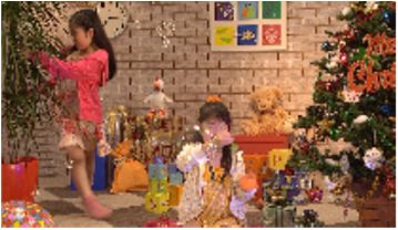
7.3    More visual results
We illustrate more visual results in Figure 15 (on the last page), which
shows both spatial textures and temporal profiles of the proposed PLVC                 LPIPS on JCT-VC (average among all GOPs)
approach, HEVC (HM 16.20) and RLVC (MS-SSIM) [Yang et al.,                      0.12
                                                                                                                           P-frame   1
2021], in addition to Figure 5 in the main text. It can be seen from Fig-                                                  P-frame   2
                                                                                0.11
ure 15, the proposed PLVC approach achieves more detailed and sharp                                                        P-frame   3
textures than other methods, even if when HEVC consumes obviously                                                          P-frame   4
                                                                                0.10                                       P-frame   5
more bit-rates and RLVC consumes more than 2× bits. Besides, the                                                           P-frame   6
temporal profiles also show that our PLVC approach has similar tem-             0.09                                       P-frame   7
                                                                                                                           P-frame   8
poral coherence to the groundtruth, and the temporal profiles also show         0.08
that we generate more photo-realistic textures than the compared meth-
ods. These results are consistent with the user study in Figure 6 of the        0.07
main text, validating the outstanding perceptual performance of the pro-        0.06
posed PLVC approach.
                                                                                0.05
7.4    Time complexity                                                             0.00   0.02   0.04   0.06 0.08   0.10   0.12      0.14
                                                                                                            bpp
We conduct all training and test procedures on the TITAN Xp GPU with
Debian GNU/Linux 10 system. The average encoding time on a 240p,
480p and 1080p frame is 0.063s (15.9 fps), 0.114s (8.8 fps) and 0.465s         Figure 14: The average performance on LPIPS along
                                                                               time steps in the GOPs.
(2.2fps), respectively. The average decoding time on a 240p, 480p and
1080p frame is 0.031s (32.3 fps), 0.065s (15.4 fps) and 0.371s (2.7 fps),
respectively. The training time of one model (including the warm up by
MSE loss) takes around 170 hours.

8     Video examples
We provide same examples of compressed videos for a direct visual comparison in the folder “Video examples” in the Project
Page at https://github.com/RenYang-home/PLVC. The files and the corresponding methods/models are listed in Table 2. The
subfolder “Examples” include the video examples of the proposed PLVC approach, HM 16.20 and the MS-SSIM-optimized
RLVC [Yang et al., 2021]. The subfolder “Examples (ablation)” includes the results of the ablation models on the same video
as “Examples”, so the ablation results should be compared with the result of our PLVC approach in “Examples”.
                               Table 2: The files and corresponding methods/models in video examples.
           Examples
           1. Our PLVC bpp=xxx.mkv                       The proposed PLVC method
           2. RLVC (SSIM) bpp=xxx.mkv                    The MS-SSIM-optimized RLVC method [Yang et al., 2021]
           3. HM16.20 bpp=xxx.bin                        The official HEVC test model HM 16.20
           Examples (ablation)
           4. PLVC (no hˆD, no m i) bpp=xxx.mkv          PLVC (w/o hD
                                                                    i , w/o mi in D)
           5. PLVC (no GAN) bpp=xxx.mkv                  PLVC (w/o GAN)

   Due to the size limitation, we show the first 100 frames of each method, and in the ablation video examples, we show the
results of the two most important models PLVC (w/o hD   i , w/o mi in D) and PLVC (w/o GAN), which verify the effectiveness
the proposed temporal condition in the discriminator and the effectiveness of the proposed GAN-based approach, respectively.
Besides, since storing the compressed frames in PNG format significantly exceeds the size limitation, we first obtain the
compressed frames of each model and then near-losslessly re-compress the frames by x265 as “.mkv” files to reduce the file
size. For HM 16.20, we directly provide the bitstream (“.bin” file) to save the space.
   Note that, due to the near-losslessly re-compression by x265 for the “.mkv” files, the file sizes of the “.mkv” files do not
indicate the bit-rate of the proposed and compared methods. The bit-rates are directly written in the file names. The
“.mkv” files can be displayed by the VLC media player (https://www.videolan.org/index.zh.html). Note that since we store the
compressed frames and then near-losslessly compress them by x265, the file sizes of the “.mkv” files do not indicate the bit-rate
of the proposed and compared methods. The bit-rates are directly written in the file names. The “.bin” file of HM 16.20 can be
viewed by the standard HEVC decoder, e.g., HM decoder.

9     Codes and reproducibility
To ensure the reproducibility, we will release all training and test codes with pre-trained models at https://github.com/
RenYang-home/PLVC.
10    Broader impact and ethics statement
The generative video compression aims at compressing videos at low bit-rates and with good perceptual quality, which highly
correlated with the Quality of Experience (QoE). Therefore, the study on perceptual video compression is meaningful for the
efficient video transmission over the Internet with satisfied QoE.
   Besides, since the traditional video coding standards, e.g., HEVC, have been developed for several decades and are very well
designed, the previous PSNR-optimized learned video compression methods are hard to compete with HM 16.20 in terms of
PSNR. Thus, it is important to further explore the advantage of deep networks to seek a promising way to surpass the traditional
codecs. The generative adversarial network and the adversarial training strategy are the strengths of deep learning, which can
not be achieved by the handcrafted architectures. Therefore, the study on generative video compression plays to the strengths
of deep networks, thus making it a promising direction to outperform the traditional video coding standards.
   As far as we know, there is no ethical issues on the proposed method and the datasets in this paper.
Groundtruth           Proposed PLVC        HEVC (HM 16.20)         RLVC (MS-SSIM)
                                                                bpp = 0.027       bpp = 0.028 (~1.04×)    bpp = 0.062 (~2.3×)

                                         Groundtruth          Proposed PLVC         HEVC (HM 16.20)        RLVC (MS-SSIM)
                                                                bpp = 0.062        bpp = 0.095 (~1.5×)    bpp = 0.131 (~2.1×)

                                        Groundtruth          Proposed PLVC         HEVC (HM 16.20)        RLVC (MS-SSIM)
                                                               bpp = 0.013        bpp = 0.021 (~1.6×)    bpp = 0.079 (~6.1×)

                                         Groundtruth          Proposed PLVC         HEVC (HM 16.20)        RLVC (MS-SSIM)
                                                                bpp = 0.027        bpp = 0.044 (~1.6×)    bpp = 0.077 (~2.9×)

Figure 15: The visual results of the proposed PLVC approach in comparison with HM 16.20 and the MS-SSIM optimized RLVC [Yang et
al., 2021]
You can also read