Performance of the GenEst Mortality Estimator Compared to the Huso and Shoenfeld Estimators - AWWI TECHNICAL REPORT

AWWI TECHNICAL REPORT

Performance
of the GenEst
Mortality Estimator
Compared to the
Huso and Shoenfeld
Estimators
Prepared by:
Paul A Rabie, Daniel Riser-Espinoza, Jared Studyvin, Daniel
Dalthorp, Manuela Huso

March 10, 2021

Performance of the GenEst Statistical Mortality Estimator

AWWI Technical Report:

Performance of the GenEst Mortality Estimator
Compared to the Huso and Shoenfeld Estimators
American Wind Wildlife Institute
1990 K Street NW, Suite 620
Washington, DC 20006
www.awwi.org

For Release March 10, 2021

AWWI is a partnership of leaders in the wind industry, wildlife management agencies, and science and
environmental organizations who collaborate on a shared mission: to facilitate timely and responsible
development of wind energy while protecting wildlife and wildlife habitat.

Find this document online at www.awwi.org/resources/genest/

Acknowledgments

The authors thank Kristen Nasman, Andrew Tredennick, John Lloyd, and Taber Allison for their helpful
comments on earlier drafts of this report, and AWWI for facilitating the project. Financial support for this
work was provided by the American Wind Wildlife Institute, the National Renewable Energy Laboratory,
and U.S. Department of Energy’s Office of Energy Efficiency and Renewable Energy under the Wind Energy
Technologies Office.

Prepared By
Western EcoSystems Technology, Inc.
 Paul A Rabie
 Daniel Riser-Espinoza
 Jared Studyvin
U.S. Geological Survey Forest & Rangeland Ecosystem Science Center
 Daniel Dalthorp
 Manuela Huso

Suggested Citation Format
Rabie, P. A., D. Riser-Espinoza, J. Studyvin, D. Dalthorp, and M. Huso. 2021. AWWI Technical Report:
Performance of the GenEst Mortality Estimator Compared to the Huso and Shoenfeld Estimators.
Washington, DC. Available at www.awwi.org. © 2020 American Wind Wildlife Institute.

March 10, 2021 1

Performance of the GenEst Statistical Mortality Estimator

Contents
1. Introduction ...................................................................................................................................................... 5

2. Methods ........................................................................................................................................................... 6

 2.1 Mortality Estimation Components............................................................................................................ 6

 2.2 Estimator Variants .................................................................................................................................... 7

 2.3 Simulation Conditions .............................................................................................................................. 8

 2.4 Estimator Implementation ........................................................................................................................ 9

 2.5 Estimator Assessment ........................................................................................................................... 10

3. Results ............................................................................................................................................................ 10

 3.1 Bias .......................................................................................................................................................... 10

 3.2 Confidence Interval Coverage ................................................................................................................ 14

 3.3 Precision and Confidence Interval Coverage ........................................................................................ 18

4. Implications for the Analysis and Design of Post-construction Monitoring Studies.................................26

5. References ..................................................................................................................................................... 28

March 10, 2021 2

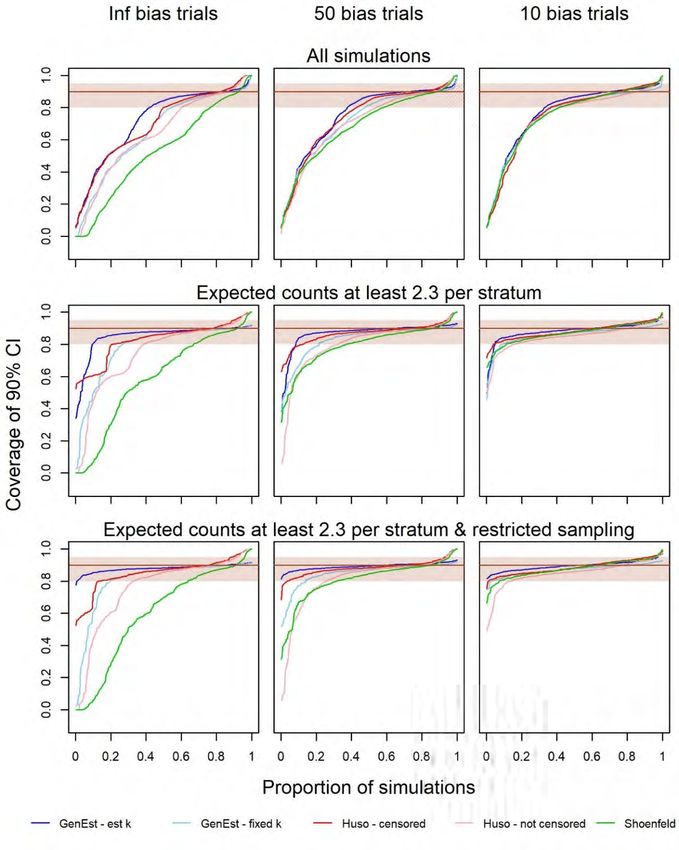
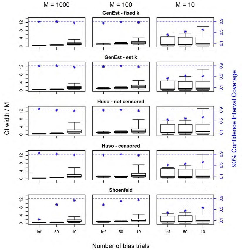
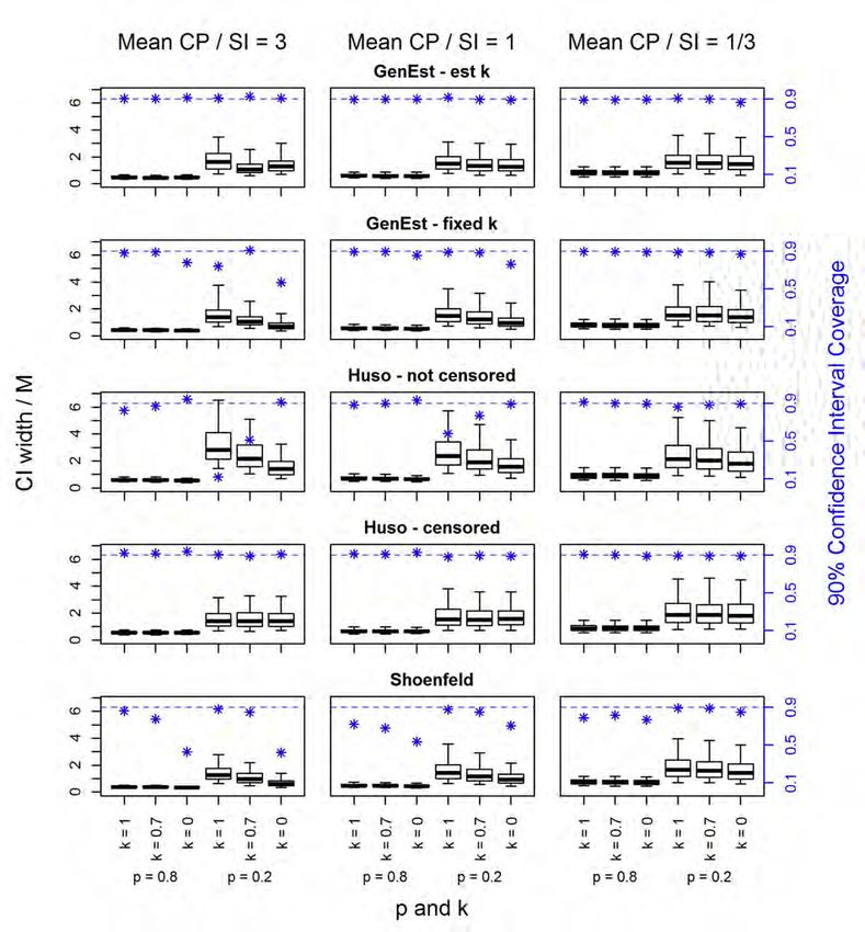
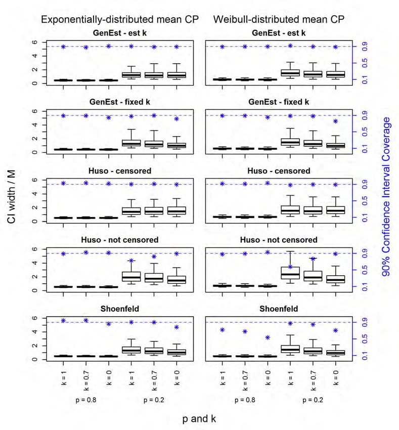
Performance of the GenEst Statistical Mortality Estimator

Tables
Table 1. Factors, their values used in the simulations, and their descriptions....................................... 8

Table 2. Parameter values and modeled detection probabilities for the five estimators,
 where p refers to initial searcher efficiency and k to the detection reduction
 factor. Persistence distributions are parameterized as in the base R software.
 Mean CP:SI is the mean carcass persistence time (itself a function of the
 persistence distribution) divided by the search interval (seven days in all cases).
 Mean CP:SI less than 1.0 implies the search interval is longer than the mean
 persistence time, while a mean CP:SI greater than 1.0 implies the search interval
 is shorter than the mean persistence time............................................................................... 11

Figures
Figure 1. Relative bias of the five estimators under the 36 core scenarios that result in
 different detection probabilities. Within each panel, the x-axis repeats the k values
 twice. The y-axis has been log-transformed so that an underestimate by a factor
 of 2 is visually similar to an overestimate by a factor of 2. The reference line at
 1.0 indicates an unbiased estimator, points above the line suggest estimators
 that are biased high, and points below the line suggest estimators that are biased
 low. Dotted reference lines indicate estimates that are 0.8 and 1.2 times the
 unbiased value. .......................................................................................................................... 15

Figure 2. Confidence interval (CI) coverage of the five estimators under different bias trial
 sample sizes (in columns). Within each panel, the realized coverage is plotted
 from low to high across all simulations conducted. Nominal coverage is indicated
 with a brown line at 0.9 and the shaded region includes coverage from 0.8 to
 0.95. The top row of panels includes all simulations, the second row excludes
 simulations for which the expected carcass count was less than 2.3 per stratum
 (road and pad or cleared plots), and the third row additionally excludes
 simulations with sampling inadequate to capture the variability in mortality rates
 across the facility (see text). ..................................................................................................... 16

Figure 3. Precision and confidence interval (CI) coverage of mortality estimates in
 response to total mortality and sample size for bias trials. Boxplots show the
 median (horizontal bar), 25th and 75th quantiles (lower and upper bounds of the
 boxes) and 5th and 95th quantiles (whiskers) of the widths of 90% CI for mortality
 estimates. CI coverage is indicated in blue on the right axis and with asterisks,
 with a reference line indicating 90% coverage. The figure includes simulations for
 which there was a gradient of mortality across the 100-turbine wind facility.
 Sampling fraction was 100%, with 30% of turbines searched as cleared plots and
 70% as road and pads, p = 0.8, k = 0.7, and carcass persistence was Weibull
 distributed with the mean persistence time equal to the search interval. .............................20

Figure 4. Precision and coverage of mortality estimates due to the carcass persistence
 time distribution, k and p. Boxplot interpretation as in Figure 3. The figure
 includes simulations for which total fatality was 1,000 individuals with a gradient
 of mortality across the 100-turbine wind facility. Sampling fraction was 100%,
 with 30% of turbines searched as cleared plots and 70% as road and pads. Mean

March 10, 2021 3

Performance of the GenEst Statistical Mortality Estimator

 carcass persistence time was equal to the search interval. There were 50 bias
 trial carcasses available to estimate model parameters. .......................................................21

Figure 5. Precision and coverage of mortality estimates due to the length of the mean
 carcass persistence time relative to the search interval, k and p. Boxplot
 interpretation as in Figure 3. The figure includes simulations for which total
 fatality was 1,000 individuals with a gradient of mortality across the 100-turbine
 wind facility. Sampling fraction was 100%, with 30% of turbines searched as
 cleared plots and 70% as road and pads; carcass persistence was Weibull
 distributed. There were 50 bias trial carcasses available to estimate model
 parameters. ................................................................................................................................ 22

Figure 6. Precision and coverage of mortality estimates due to spatial distribution of
 fatalities, sampling fraction, and total number of turbines at the facility. Boxplot
 interpretation as in Figure 3. The figure includes simulations for which total
 fatality was 1,000 individuals. Thirty percent of searched turbines were searched
 as cleared plots and 70% as road and pads, p = 0.8, k = 0.7, and carcass
 persistence was Weibull-distributed with mean persistence time equal to the
 search interval. There were 50 bias trial carcasses available to estimate model
 parameters. ................................................................................................................................ 24

Figure 7. Precision and coverage of mortality estimates due to the plot configuration,
 sampling fraction, and total number of turbines at the facility. Boxplot
 interpretation as in Figure 3. The figure includes simulations for which total
 fatality was 1,000 individuals with a gradient of mortality across the wind facility,
 p = 0.8, k = 0.7, and carcass persistence was Weibull-distributed with the mean
 persistence time equal to the search interval. There were 50 bias trial carcasses
 available to estimate model parameters. ................................................................................. 25

March 10, 2021 4

Performance of the GenEst Statistical Mortality Estimator

1. Introduction
The impacts of wind power development on bat and bird populations are commonly assessed by
estimating the number of fatalities at wind power facilities through post-construction monitoring (PCM)
studies. Standard methodology involves periodic carcass searches on plots beneath turbines (Strickland
et al. 2011, US Fish and Wildlife Service 2012). The resulting counts are adjusted to compensate for bias
due to imperfect carcass detection by searchers, removal of carcasses by scavengers or other processes
(Korner-Nievergelt et al. 2011), and carcasses that may have fallen outside of searched areas. To account
for the bias in counts due to imperfect detection and carcass removal, investigators typically conduct
bias trial experiments to inform models of carcass detection probability. Many different estimators have
been proposed that combine information about the bias trial experiments to estimate a detection
probability for carcasses (g) and ultimately obtain an estimate of total mortality (M). The two estimators
that have seen the most widespread use in North America recently are the Huso (Huso 2011, Huso et al.
2012) and Shoenfeld (Shoenfeld 2004; also called the Erickson estimator) estimators. GenEst (Dalthorp
et al. 2018a, 2018b, 2018c) is the newest statistical estimator to become available and was designed to
improve upon the Huso and Shoenfeld estimators by generalizing the key assumptions in both, and to
improve comparability among new PCM studies. In addition to relaxing some of the assumptions inherent
in the Huso and Shoenfeld estimators, GenEst uses a novel approach to variance estimation through a
parametric bootstrap (Madsen et al. 2019).

The current study was undertaken to document the performance of GenEst relative to the Huso and
Shoenfeld estimators. We took a simulation approach to the study because simulation data provides the
basis to compare mortality estimators under conditions where the “truth” is known. The estimators were
compared on three metrics: 1) bias—the tendency of an estimator to over- or under-estimate mortality, 2)
precision—the ability of an estimator to constrain an estimate to a narrow range (measured here as the
width of a 90% confidence interval [CI] around the point estimate divided by the true, known mortality
rate), and 3) CI coverage—the probability a CI with a specified level of confidence actually includes the
true level of mortality.

Although our simulations were conceived and designed—and are discussed—with respect to wind farms,
it is important to note that the estimators and results discussed here are relevant to any post-
construction mortality monitoring study that may occur (such as at solar facilities) where detection is
imperfect. Although our study treats the problem of mortality estimation when detection is imperfect, it is
also important to note that all of the estimators considered here are Horvitz-Thompson-style estimators
(Horvitz and Thompson 1952), that is, none are designed to estimate the mortality of rare species as
might be necessary under an Incidental Take Permit. The Evidence of Absence estimator (Dalthorp et al.
2017) is still the most appropriate statistical tool for rare event estimation.

The simulations cover a broad range of conditions that may occur in field studies and complete results
are presented without commentary in the appendix. The main body of this report does not provide a
comprehensive treatment of our results; rather, we try to identify some of the more important differences
among the estimators and some conditions under which reliable mortality estimates are especially
challenging.

March 10, 2021 5

Performance of the GenEst Statistical Mortality Estimator

2. Methods
2.1 Mortality Estimation Components
All of the estimators treated here address four or five of the same components of carcass detection
probability to arrive at an estimate of total mortality and differ primarily in the assumptions associated
with the components of detection probability. We begin with a brief review of these components.

The carcass persistence (CP) probability addresses the potential bias in carcass counts due to the fact
that a carcass may be removed by a scavenger (or another process) before a searcher completes a
monitoring survey. The GenEst and Huso estimators both use survival-modeling techniques to estimate a
distribution of carcass persistence times, from which the average persistence probability can be
calculated. These estimators provide the user with tools to help choose among different distributions for
carcass persistence times, which makes them flexible with respect to the carcass persistence dynamics.
The Shoenfeld estimator implicitly assumes carcass persistence times follow an exponential distribution.
When persistence times do not meet this assumption, the Shoenfeld estimator can be biased.

Searcher efficiency (SE) addresses the bias that arises from imperfect detection of carcasses by
searchers. All of the estimators tested here take an initial searcher efficiency parameter (p), which may
differ from season to season or between substrate strata at a wind farm. Searcher efficiency also
depends on carcass age, as carcasses tend to become more difficult to discover as they age, and k
describes how searcher efficiency changes as carcasses age. Carcasses newly arrived at a facility may
be detected with probability p (above) or may be missed. Those carcasses that are missed may begin to
disintegrate and become harder to detect, or may have been well concealed in the first place, so it is
reasonable to expect that a carcass that has been missed once will have a lower detection probability
than a fresh carcass. The k parameter describes how searcher efficiency changes through multiple
searches.

Shoenfeld assumes searcher efficiency does not depend on carcass age ( = 1). Huso assumes
carcasses that are not discovered in the first search after arrival cannot be discovered in later searches,
i.e., searcher efficiency goes to zero for carcasses missed in the first search ( = 0). Among the
estimators tested here, only GenEst treats k explicitly. GenEst uses a maximum likelihood procedure to
estimate p simultaneously with k, if there are multiple search data available (as in our GenEst-est k
estimations below). If there are only single-search data available, the GenEst estimation routine to
estimate p reduces to a logistic regression and the user must specify a value (between zero and one) for
k (as in our GenEst-fixed k simulations below, which used a fixed value of 0.7 for k). Choosing fixed k = 1
is equivalent to the Shoenfeld approach to modeling searcher efficiency and choosing fixed k = 0 is
equivalent to the Huso approach. The Huso estimator uses logistic regression to estimate p, and
although there is no canonical approach to estimating p for the Shoenfeld estimator, logistic regression is
a reasonable choice and was used here.

The estimators behave differently when presented with a data set for which either all or none of the
searcher efficiency trial carcasses are detected. When no searcher efficiency trial carcasses are detected
by searchers, the Shoenfeld and Huso estimators are unable to produce a mortality estimate because
with p = 0, estimated mortality would be infinite, which is nonsensical. In contrast, the GenEst estimator
(version 1.3.1 and later) uses an estimate of 1 / (2 * n) when no searcher efficiency trial carcasses are
detected (e.g., if all of 10 carcasses are missed, GenEst will use an assumed value of 1/20 for p).
Although this assumption introduces an unknown bias to the estimator, it allows GenEst to produce
mortality estimates where other estimators fail. When all searcher efficiency trial carcasses are detected
by searchers, the Shoenfeld and Huso estimators proceed with a searcher efficiency estimate of 1.0,
which is also implausible and introduces an unknown bias, but perhaps not an unreasonable
approximation of reality if the number of trial carcasses is large. Analogous to the zero-found case, the

March 10, 2021 6

Performance of the GenEst Statistical Mortality Estimator

GenEst estimator (as of version 1.3.1) assumes searcher efficiency is 1 - 1 / (2 * n) when all carcasses
are found (e.g., if all of 10 trial carcasses are detected, GenEst will use an assumed value of 19/20 for p).
This assumption introduces an unknown bias to the estimator, but in most cases will be less biased than
simply assuming p = 1 and gives a more realistic assessment of the uncertainty in the estimate of p (and
total mortality) when all searcher efficiency carcasses are detected.

A final important difference between the estimators is the treatment of uncertainty. Shoenfeld (2003) did
not address uncertainty in the estimator. The Huso estimator uses a non-parametric bootstrap (i.e., a
data-resampling procedure) to capture uncertainty in the detection probability and carcass counts, and
we use the same approach for the Shoenfeld estimator. The GenEst estimator uses a parametric
bootstrap procedure to capture uncertainty in the detection probability and carcass counts. For detection
probability, this means parameter estimates are resampled based on the estimated uncertainty in the
model; for carcass counts, the parametric bootstrap represents a completely novel approach developed
specifically for the GenEst model (though it potentially has much wider application; Madsen et al. 2019).
A consequence of the parametric bootstrap used by GenEst is that, rather than the turbine being a
statistical sample unit (as in the Huso and Shoenfeld estimators), the carcass is the sample unit, which
frees GenEst from the assumption that mortality rates are constant among turbines and makes it
applicable across a broader range of conditions.

Differences in the way carcass persistence, searcher efficiency, k, and uncertainty are treated mark the
most fundamental differences between the estimators tested here. However, two other components of
mortality estimation are also important and were included in our simulation. Sampling fraction refers to
the fraction of wind turbines at a farm actually subject to search and is an important indicator of the
actual sampling effort. The sampling effort also depends on plot configurations. Large, cleared plots may
be expected to capture most carcasses that arrive at a wind farm, whereas road and pad searches that
are restricted to the graveled surfaces around wind turbines may capture a small fraction of the total
carcasses that arrive. The fraction of carcasses expected to occur within searched areas is called the
density-weighted proportion of area searched, or DWP.

The estimated detection probabilities for all of the estimators treated here are adjusted after the fact to
account for sampling fraction and DWP. Post hoc adjustment for sampling fraction and DWP means their
effects on the point estimates of mortality scale linearly with sampling fraction and DWP, but because the
different estimators handle uncertainty associated with carcass counts differently, these factors can
impact precision and CI coverage differently for the different estimators.

2.2 Estimator Variants
The study tested estimator performance of five estimator variants (italicized below) under a variety of
simulated conditions (Table 1). Three estimators were tested: the GenEst estimator (as in version 1.4.2 of
the software), the Huso estimator, and the Shoenfeld estimator. GenEst has the capacity to estimate the
proportional change in searcher efficiency with each successive search (k) or to treat it as fixed and
known. For the GenEst-est k case, we estimated k from simulated bias trial data. For the GenEst-fixed k
case, we assumed k was equal to 0.7, regardless of its actual value. The Huso estimator includes the
implicit assumption that k is zero, which is to say it assumes that if a carcass is missed once it will never
be detected. Carcass search data can be prepared to approximate this assumption by restricting the
carcass counts to only those carcasses that are ‘fresh,’ i.e., occurred since the last search. The notion
that carcasses can be censored to satisfy the assumptions of the Huso estimator is simple in principle,
but it bears emphasizing that in the field, the task of censoring carcasses is influenced by a great deal of
subjective judgment, and accuracy in the censoring process remains untested. Huso-censored estimates
were calculated using carcass counts identified as fresh (with perfect accuracy), and Huso-not censored
estimates used all carcasses in the estimates. Neither of our Huso variants is likely to be the case in the
field, but they represent a range of potential outcomes. The Shoenfeld estimator makes the implicit
assumption that k is 1.0, which means the detection probability for a carcass never changes, regardless

March 10, 2021 7

Performance of the GenEst Statistical Mortality Estimator

of how many times it has been missed. Unlike the Huso estimator, there is no way to prepare the data so
that it matches the implicit assumptions of the Shoenfeld estimator. Thus, the three basic estimators
resulted in five types of mortality estimates: GenEst-est k, GenEst-fixed k, Huso-censored, Huso-not
censored, and Shoenfeld.

2.3 Simulation Conditions
Several factors affect the performance of these estimators. The factors that we consider are total
mortality at a site, whether the mortality is evenly distributed among turbines or varies among turbines,
the number of turbines at a site, the sampling fraction, the DWP (which depends on plot configuration),
the carcass persistence distribution, the length of the search interval relative to the average carcass
persistence time, the searcher efficiency, the value of k, and, finally, the number of trial carcasses used to
estimate p, k, and carcass persistence.

Each estimator was tested in the context of simulated mortality monitoring studies at a wind facility. The
simulated studies covered 26 weeks with the search interval fixed at seven days. All simulated fatalities
were assumed to be from the same class of animal in terms of detection and persistence probability (i.e.,
all bats or all similarly sized birds). The total number of fatalities arriving at the wind facility, carcass
persistence distribution, mean persistence time, searcher efficiency, number of bias trial carcasses,
distribution of fatalities across the wind facility, and k were varied systematically across the simulations—
see Table 1 for a description of all conditions tested during simulations. All combinations of conditions in
Table 1 were simulated for each estimator, except for the combination of a uniform distribution of total
mortality = 10 at a site with 100 turbines, because it is impossible to uniformly distribute 10 whole
carcasses across 100 turbines. There were 4,752 simulation scenarios to which each of the five
estimators was applied. A carcass count and bias trial data were generated 1000 times for each of the
4,752 scenarios. For each carcass count, each estimator gave a point estimate of mortality ( � ) and a 90%
CI around �.

Table 1. Factors, their values used in the simulations, and their descriptions.

Factor Levels Description

Total mortality M = 1000 Total number of carcasses distributed at simulated wind
(M) at a site M = 100 facilities.
 M = 10

Spatial Uniform M Uniform M distribution indicates the case where the mortality
distribution of rates are identical for all turbines at a facility.
mortality

 Variable M Variable M distribution indicates the case where the mortality
 rates at turbines within a wind facility included a five-fold
 variation from the least lethal turbine to the most lethal
 turbine.

Number of 100 turbines Number of turbines over which to distribute total fatalities.
turbines 10 turbines

Sampling fraction f = 1.0 Proportion of total turbines at a facility that were searched.
(f) f = 0.3

March 10, 2021 8

Performance of the GenEst Statistical Mortality Estimator

Plot Plot type = Cleared Plot configuration for searches involved either cleared plots
configurations Plot type = Cleared + RP at all searched turbines (assumed large enough to capture all
 carcasses) or a mixture of 30% cleared plots and 70% of
 turbines searched on road and pads (large enough to capture
 15% of carcasses).

Carcass Exponential Carcass persistence times followed either an exponential
persistence time Weibull distribution or a Weibull distribution with a shape parameter
distribution1 equal to 0.6.

Ratio of average Mean CP:SI = 1/3 Ratio of average carcass persistence time: length of search
persistence time Mean CP:SI = 1 interval; these resulted in the probability of persisting through
to search interval Mean CP:SI = 3 the search interval (r) being 21%, 33% and 27% higher for the
 exponential than Weibull, respectively.

Searcher p = 0.8 Probability a fresh carcass will be detected on a search,
efficiency for a p = 0.2 assuming it has not been removed.
fresh carcass

Detection k=0 Fraction by which searcher efficiency for an aging carcass
reduction factor k = 0.7 decreases with each successive search.
(k) k = 1.0

Number (N) of N bias trials = Infinite Mortality estimators are informed by bias trials to estimate
bias trial N bias trials = 50 searcher efficiency, carcass persistence (and for GenEst, k).
carcasses N bias trials = 10 We simulated 10 or 50 bias trials, and the ideal case where
 components of bias were known with certainty
 (N bias trials = infinite).

Estimator GenEst-est k See text above.
 GenEst-fixed k
 Huso-censored
 Huso-not censored
 Shoenfeld

2.4 Estimator Implementation
Estimates and CIs (parametric) for GenEst-est k and GenEst-fixed k were generated using version 1.4.2 of
the GenEst R package. For the Huso-censored and Huso-not censored, estimates and CIs were generated
using R code adapted from US Geological Survey Data Series 729 (Huso et al. 2012), and, thus, replicate
the expected behavior of the Huso estimator as implemented in Data Series 729. There is no R package
or publicly available software for implementing the Shoenfeld estimator, and critical details of the
implementation of the estimator can vary considerably from project to project. The estimates for
Shoenfeld were generated using R code developed by WEST based on Shoenfeld (2004). CIs for the Huso
and Shoenfeld estimators were generated using a non-parametric bootstrap approach similar to that
used in Data Series 729. For the Huso and Shoenfeld estimator variants, no estimate was produced for a
simulation iteration when zero searcher efficiency carcasses were found on the first search of the
associated simulated bias trials, although in DS 729 a minimum SE of 1/20 is assumed in such cases.
GenEst version 1.3.1 and later assumes p = 1 / (2 * n) in these cases.

March 10, 2021 9

Performance of the GenEst Statistical Mortality Estimator

2.5 Estimator Assessment
Estimator performance was assessed based on three metrics: CI coverage, relative bias, and precision. CI
coverage is calculated as the proportion of the 1000 simulated 90% CIs around the estimated mortality,
 � , that contain the true mortality, . That the 90% CI actually achieve nominal coverage, i.e., that it
 
includes 90% of the time, is important for correct interpretation of results. A 90% CI that contains the
true 100% of the time would be easy to construct, e.g., is between what was found and some very
large number, 1,000,000 say, but would be of little practical value. Conversely, a very narrow CI might look
appealing from a precision perspective, but, again, would be of little value if it never included the true
value of M. The relative bias is calculated as the estimated mortality ( � ) divided by the true mortality ( ).
The ratio equals 1.0 when the estimate is identical to the true mortality, is greater than 1.0 for estimates
above the true , and less than 1.0 for estimates below the true . Relative bias of ½ is equivalent to bias
of 2 in terms of how far the estimator misses the mark. Precision is calculated as the width of the 90% CI
around the estimate of divided by the true mortality, . We chose to standardize this metric,
analogously to a coefficient of variation, to facilitate comparison of precision across different levels of
true mortality.

None of the three metrics can be interpreted well by itself. For example, an estimator may be unbiased,
i.e., its average value over the 1000 iterations is exactly the true mortality, but it may also be very
imprecise with 90% CIs so large that they cover the true mortality 100% of the time. An estimator with this
characteristic is unlikely to be of practical use. An estimator may, on the other hand, be extremely precise,
but the 90% CIs are so narrow that they rarely include the true mortality. The best estimator will be one
that is consistently accurate (relative bias = 1), precise, and achieves nominal coverage. To present the
results in a manageable way, we begin with a discussion of the inherent biases of the estimators,
followed by a high-level overview of CI coverage, and finally a series of results for which we discuss
precision and coverage simultaneously.

3. Results
3.1 Bias
The Huso, GenEst, and Shoenfeld estimators differ most profoundly in the parameters used in estimating
overall detection probability, and the assumptions on which those detection probability models are based.
We begin by analyzing the 36 core scenarios that include all combinations of the searcher efficiency, k,
and carcass persistence parameters that we investigated. For this analysis, we ignore the factors that
primarily affect the assessments of uncertainty (total mortality, the spatial dispersion of carcasses
among turbines, the number of turbines, and the number of field trial carcasses) and the extrapolation
factors (DWP and sampling fraction), which the three estimators handle in similar ways.

Table 2 gives the modeled probability of detection ( ) for each of the five estimators, assuming the
sampling fraction and density-weighted proportion of carcasses are both 1.0 under the 36 core scenarios.
The 36 unique simulation scenarios derive from two levels of searcher efficiency (0.2 and 0.8), three
levels of k (0, 0.7 and 1.0), two carcass persistence distributions (exponential and Weibull), and three
mean carcass persistence times relative to the search interval (1/3, 1, 3). The modeled detection
probabilities for GenEst with known k and for Huso with perfect carcass censoring are exactly correct, but
they differ from one another when k is not zero because they assume different data collection procedures
in the field. The Huso estimator is unbiased when k = 0 or when carcasses are accurately censored, but
 
biased by a factor of when k is greater than zero and carcasses are not censored.
 
March 10, 2021 10

Performance of the GenEst Statistical Mortality Estimator

Table 2. Parameter values and modeled detection probabilities for the five estimators, where p refers to initial searcher efficiency and k to the
detection reduction factor. Persistence distributions are parameterized as in the base R software. Mean CP:SI is the mean carcass persistence time
(itself a function of the persistence distribution) divided by the search interval (seven days in all cases). Mean CP:SI less than 1.0 implies the search
interval is longer than the mean persistence time, while a mean CP:SI greater than 1.0 implies the search interval is shorter than the mean
persistence time.

 Estimator parameters Modeled detection probabilities

 p k Persistence distribution (parameters) Mean CP:SI GenEst-k
 assumed to be Huso (both
 GenEst-k known 0.7 variants) Shoenfeld

0.8 1.0 exponential (rate = 0.0476) 3.00 0.789 0.766 0.680 0.794

0.8 1.0 exponential (rate = 0.1429) 1.00 0.544 0.534 0.506 0.546

0.8 1.0 exponential (rate = 0.4286) 0.33 0.256 0.255 0.253 0.256

0.8 1.0 Weibull (shape = 0.6; scale = 13.9574) 3.00 0.615 0.599 0.537 0.794

0.8 1.0 Weibull (shape = 0.6; scale = 4.6525) 1.00 0.415 0.406 0.380 0.546

0.8 1.0 Weibull (shape = 0.6; scale = 1.5287) 0.33 0.217 0.215 0.210 0.256

0.8 0.7 exponential (rate = 0.0476) 3.00 0.766 0.766 0.68 0.794

0.8 0.7 exponential (rate = 0.1429) 1.00 0.534 0.534 0.506 0.546

0.8 0.7 exponential (rate = 0.4286) 0.33 0.255 0.255 0.253 0.256

0.8 0.7 Weibull (shape = 0.6; scale = 13.9574) 3.00 0.599 0.599 0.537 0.794

0.8 0.7 Weibull (shape = 0.6; scale = 4.6525) 1.00 0.406 0.406 0.380 0.546

0.8 0.7 Weibull (shape = 0.6; scale = 1.5287) 0.33 0.215 0.215 0.210 0.256

0.8 0 exponential (rate = 0.0476) 3.00 0.680 0.766 0.680 0.794

March 10, 2021 11

Performance of the GenEst Statistical Mortality Estimator

 Estimator parameters Modeled detection probabilities

 p k Persistence distribution (parameters) Mean CP:SI GenEst-k
 assumed to be Huso (both
 GenEst-k known 0.7 variants) Shoenfeld

0.8 0 exponential (rate = 0.1429) 1.00 0.506 0.534 0.506 0.546

0.8 0 exponential (rate = 0.4286) 0.33 0.253 0.255 0.253 0.256

0.8 0 Weibull (shape = 0.6; scale = 13.9574) 3.00 0.537 0.599 0.537 0.794

0.8 0 Weibull (shape = 0.6; scale = 4.6525) 1.00 0.380 0.406 0.380 0.546

0.8 0 Weibull (shape = 0.6; scale = 1.5287) 0.33 0.210 0.215 0.210 0.256

0.2 1.0 exponential (rate = 0.0476) 3.00 0.378 0.284 0.170 0.399

0.2 1.0 exponential (rate = 0.1429) 1.00 0.176 0.158 0.126 0.179

0.2 1.0 exponential (rate = 0.4286) 0.33 0.066 0.065 0.063 0.066

0.2 1.0 Weibull (shape = 0.6; scale = 13.9574) 3.00 0.298 0.220 0.134 0.399

0.2 1.0 Weibull (shape = 0.6; scale = 4.6525) 1.00 0.151 0.128 0.095 0.179

0.2 1.0 Weibull (shape = 0.6; scale = 1.5287) 0.33 0.062 0.059 0.052 0.066

0.2 0.7 exponential (rate = 0.0476) 3.00 0.284 0.284 0.170 0.399

0.2 0.7 exponential (rate = 0.1429) 1.00 0.158 0.158 0.126 0.179

0.2 0.7 exponential (rate = 0.4286) 0.33 0.065 0.065 0.063 0.066

0.2 0.7 Weibull (shape = 0.6; scale = 13.9574) 3.00 0.220 0.220 0.134 0.399

0.2 0.7 Weibull (shape = 0.6; scale = 4.6525) 1.00 0.128 0.128 0.095 0.179

March 10, 2021 12

Performance of the GenEst Statistical Mortality Estimator

 Estimator parameters Modeled detection probabilities

 p k Persistence distribution (parameters) Mean CP:SI GenEst-k
 assumed to be Huso (both
 GenEst-k known 0.7 variants) Shoenfeld

0.2 0.7 Weibull (shape = 0.6; scale = 1.5287) 0.33 0.059 0.059 0.052 0.066

0.2 0 exponential (rate = 0.0476) 3.00 0.170 0.284 0.170 0.399

0.2 0 exponential (rate = 0.1429) 1.00 0.126 0.158 0.126 0.179

0.2 0 exponential (rate = 0.4286) 0.33 0.063 0.065 0.063 0.066

0.2 0 Weibull (shape = 0.6; scale = 13.9574) 3.00 0.134 0.220 0.134 0.399

0.2 0 Weibull (shape = 0.6; scale = 4.6525) 1.00 0.095 0.128 0.095 0.179

0.2 0 Weibull (shape = 0.6; scale = 1.5287) 0.33 0.052 0.059 0.052 0.066

March 10, 2021 13

Performance of the GenEst Statistical Mortality Estimator

Figure 1 shows that the GenEst-est k and the Huso-censored estimators are unbiased under all
36 combinations. GenEst-fixed k becomes biased when k is misspecified: when k is assumed higher than
the real value, GenEst-fixed k becomes biased low, and when it is assumed lower than the real value,
GenEst-fixed k becomes biased high. Low values of p and long carcass persistence times relative to the
search interval cause the greatest degree of bias in GenEst-fixed k with misspecified values of k. The
Huso-not censored estimator is unbiased only in the unlikely event that the true value of k is zero (i.e.,
there really is only one chance to detect a carcass in the field). When k is greater than zero, the Huso-not
censored estimator is biased high. Higher values of k, lower values of p, and long persistence times
relative to the search interval cause the greatest degree of bias in the Huso-not censored estimator. In
most cases, (and all cases tested here), the Shoenfeld estimator is biased low because it implicitly
assumes 1) k is 1.0, 2) carcass persistence times are exponentially distributed, and 3) each carcass is
subject to an infinite number of searches. Thus, even in the unlikely situation where k is 1.0 (i.e.,
carcasses are equally detectable after any number of searches), the Shoenfeld estimator slightly
underestimates fatalities. Underestimates are more pronounced with smaller values of k, with lower
values of p, and with shorter persistence times relative to the searcher interval. For the carcass
persistence distributions tested here, the underestimates by the Shoenfeld estimator are more
pronounced with Weibull-distributed carcass persistence times than with exponentially-distributed
carcass persistence times. This outcome is because the Weibull shape parameter we used (0.6) implies
more rapid removal of fresh carcasses compared to exponentially distributed persistence times, but this
result is not necessarily true for all possible Weibull-distributed carcass persistence dynamics.

3.2 Confidence Interval Coverage
CI coverage refers to the probability a CI will include the true value of a parameter that is being estimated.
Ideally, an estimator should produce CIs with nominal coverage—i.e., ideally a 90% CI should include the
truth with 90% probability. CI coverage greater than nominal suggests CIs are too wide. CI coverage less
than nominal can be due to estimators that are “missing” variance (CIs too narrow), or to bias (systematic
over- or under-estimation) in the estimators.

There are some easily identified conditions under which no Horvitz-Thompson estimators consistently
achieve nominal coverage. Figure 2 illustrates these. The figure is organized into three columns
according to the precision with which detection probability is estimated. In the left column (infinite bias
trials), the detection probability is known exactly and without error, the center column presents results
from simulations in which 50 bias trial carcasses were used to estimate carcass persistence and
searcher efficiency models, and the right column presents results from simulations using 10 bias trial
carcasses. In all panels, the actual CI coverage associated with simulation conditions was sorted from
low-to-high for each estimator and plotted as a line. An ideal estimator would be represented by a
horizontal line on top of the reference line at 90% CI coverage. The longer an estimator’s line is within the
shaded area (representing 80% - 95% coverage), the better its coverage property. The three rows in Figure
2 represent successive elimination of conditions under which no Horvitz-Thompson estimator can
achieve good coverage.

March 10, 2021 14

Performance of the GenEst Statistical Mortality Estimator

Figure 1. Relative bias of the five estimators under the 36 core scenarios that result in different detection
probabilities. Within each panel, the x-axis repeats the k values twice. The y-axis has been log-transformed
so that an underestimate by a factor of 2 is visually similar to an overestimate by a factor of 2. The
reference line at 1.0 indicates an unbiased estimator, points above the line suggest estimators that are
biased high, and points below the line suggest estimators that are biased low. Dotted reference lines
indicate estimates that are 0.8 and 1.2 times the unbiased value.

March 10, 2021 15

Performance of the GenEst Statistical Mortality Estimator

Figure 2. Confidence interval (CI) coverage of the five estimators under different bias trial sample sizes (in
columns). Within each panel, the realized coverage is plotted from low to high across all simulations
conducted. Nominal coverage is indicated with a brown line at 0.9 and the shaded region includes coverage
from 0.8 to 0.95. The top row of panels includes all simulations, the second row excludes simulations for
which the expected carcass count was less than 2.3 per stratum (road and pad or cleared plots), and the
third row additionally excludes simulations with sampling inadequate to capture the variability in mortality
rates across the facility (see text).

March 10, 2021 16

Performance of the GenEst Statistical Mortality Estimator

The five estimator variants in Figure 2 are easier to distinguish from one another under the theoretical-
ideal case when detection probability is known (i.e., in the left-hand panels), compared to when detection
parameters are estimated because there is less “noise.” A second pattern is that as the bias trials use
fewer carcasses, the coverages for Shoenfeld, Huso, and GenEst with fixed k tend to increase because
the uncertainties involved in estimating the SE and CP parameters when few trial carcasses are used
partially mask the problem of inherent estimator biases.

The top row of Figure 2 includes all simulation conditions, and shows that for 30–40% of the simulated
conditions none of the estimators achieved even 80% actual CI coverage with a nominal 90% CI. The
GenEst-est k estimator and Huso-censored estimators always outperformed the others, followed by the
GenEst-fixed k, Huso-not censored, and Shoenfeld estimators. It is important to note that the simulation
conditions are not necessarily a representative sample of field conditions, and some were included
precisely because they were expected to cause the estimators to fail. The second and third row of panels
in Figure 2 sequentially remove some of the most troublesome simulation conditions to illustrate their
impact on CI coverage.

All Horvitz-Thompson estimators fail under conditions of very few fatalities or very low detection
probability (Korner-Nievergelt et al. 2011) because they all produce estimates of zero mortality with no
variance when no carcasses are found. If true mortality is not zero, then these estimates will fail to cover
the true mortality, and there is an upper bound on the achievable confidence level. Considering a 90% CI:
if there is more than a 100% - 90% = 10% chance that zero carcasses will be detected, it will be impossible
to achieve 90% CI coverage with a 90% CI because at least 10% of the time the estimate is zero. It
happens that any conditions where the expected average carcass count is less than 2.3 1 are statistically
bound to under-cover a nominally 90% CI, and greater confidence levels require greater average carcass
counts (a 95% CI requires an expected count of at least 2.99). Further, for data with multiple types of
search plots (i.e., groups of plots with different detection probabilities, as occurs in data with some plots
searched as road and pads and others with cleared plots), it is necessary that the expected carcass count
be at least 2.3 in each type of search plots. Adequate expected carcass counts in all types of search plots
are necessary to ensure that the data are balanced in a way that accurately reflects the overall detection
probability for the whole study.

The second row of panels in Figure 2 is plotted after excluding all simulation cases for which the
expected carcass count is less than 2.3 in any type of search plots. For the ideal case, where bias
parameters are known (left hand panel), the coverage for GenEst-est k, Huso-censored, and GenEst-fixed k
estimators all improve markedly, Huso-not censored improves moderately, and coverage of Shoenfeld
estimates is nearly unchanged. As bias trial sample size decreases (moving right across the panels), the
coverage of the worst-performing estimators increases due to widening CI’s and the five estimators
behave more similarly to one another, though the rank-order performance (GenEst-est k>Huso-
censored>GenEst-fixed k>Huso-not censored>Shoenfeld) is maintained.

Another PCM design condition that can cause problems for estimators is a sampling strategy that is
inadequate to capture the variability in mortality from turbine to turbine across the facility. In the
simulations presented here, these conditions are present in cases where there were 1) just 10 turbines at
the wind facility, 2) a gradient of mortality among the turbines (see Spatial Distribution of Mortality in
Table 1), and 3) a sampling fraction of 30% of the turbines (i.e., just 3 turbines). In those cases, the
probability of a sample that is not representative of average conditions at the site is high.

1
 The probability that a carcass count, x, is zero, assuming x is Poisson-distributed with mean 2.3 is 0.10

March 10, 2021 17

Performance of the GenEst Statistical Mortality Estimator

The third row of panels in Figure 2 is plotted after excluding cases where the expected carcass count in
any stratum was less than 2.3 and excluding cases where there were just 10 turbines at a wind facility
with a gradient of mortality among turbines and a 30% sample of searched turbines. In this case, the
GenEst-est k estimator almost never achieves less than 80% coverage for a nominal 90% CI. To the extent
that the Huso-censored estimator underperforms GenEst-est k, it is due to differences in the way
uncertainty in counts is estimated (nonparametric bootstrap versus parametric bootstrap). To the extent
that the GenEst-fixed k estimator underperforms GenEst-est k, it is due to violations of the assumption
about the value of k. For Huso-not censored and Shoenfeld estimators, both treatment of uncertainty and
violated assumptions contribute to under-coverage.

After eliminating conditions under which no Horvitz-Thompson estimator can achieve good coverage and
where only 10 trial carcasses are used to estimate detection parameters, all the estimators achieve
coverage close to 90% in > 80% of the remaining cases, but, as discussed below, this is at a cost of
precision, i.e., wide confidence intervals.

3.3 Precision and Confidence Interval Coverage
Precision refers to the dispersion of an estimate around its point value and, in this document, is assessed
as the width of the 90% CI divided by the true mortality—a standardization that facilitates comparisons
across scenarios with greatly varying . In general, precision is useless if coverage is poor because an
estimate that is tightly constrained around the wrong answer can only mislead. Consequently, precision
and coverage are both shown on each figure in this section, and for results with poor coverage, we do not
dwell on precision.

Figures 3 through 7 are all formatted similarly. Each figure has five rows of panels with the response of
one of the estimators on each row. Each figure has two or three columns of panels that include
simulations with one level of a factor, and the x-axis of each panel includes the levels of one or two
factors from the simulation. Each panel has two y-axes; the axis on the left indicates relative width of the
 − 
90% CI (i.e., ), and the figures use boxplots to demonstrate the distribution of
 
relative CI widths obtained in the simulations. The right y-axis indicates CI coverage for the simulations
with a reference line at the nominal, 90% coverage and asterisks to indicate the coverage obtained in our
simulations. The right axis and plotting are in blue to help distinguish them from the relative CI width
information.

Precision and coverage were both strongly affected by the level of total mortality at a facility (Figure 3).
All five estimators had coverage far below the nominal 90% when total mortality was 10. As discussed in
the CI section above, these estimators are not designed to handle rare-event estimation and are known to
break down when there are few detections. Consequently, M = 10 cases are not discussed further in this
document. Of the five estimators, only the Shoenfeld estimator failed to achieve nominal coverage with M
= 100 or 1,000 carcasses, because the simulated carcass removal conditions (Weibull-distributed
removal times) do not match the assumption inherent in the Shoenfeld estimator (exponentially-
distributed removal times). For all five estimators, relative precision increased with the total mortality and
as the number of bias trial carcasses increased. Higher total mortality reduces the sampling error in the
search process, and larger sample sizes for bias trials increases the precision in the bias correction
factors, both of which lead to greater precision in the mortality estimates. The increase in precision
associated with larger bias trial sample sizes was greater as the effort increased from 10 to 50 carcasses
than as the effort increased from 50 carcasses to an infinite number (which implies bias correction
factors are known without error), suggesting diminishing returns as the number of bias trials increases
beyond 50.

Among the five estimators, only the Shoenfeld estimates had coverage that was strongly affected by the
carcass persistence time distribution (Figure 4). Most Shoenfeld estimates had coverage that was less
than nominal when carcass persistence times followed a Weibull distribution because the Weibull-

March 10, 2021 18

Performance of the GenEst Statistical Mortality Estimator

distributed persistence times violate one of the core assumptions of that estimator. Coverage of Huso-
not censored, Shoenfeld, and, to a lesser extent, GenEst-fixed k estimates was less than nominal when the
true value of k violated the estimators’ assumptions (i.e., k = 0, k = 1.0, or k = 0.7, respectively). Except for
the Shoenfeld estimates when carcass persistence time was Weibull-distributed, the effect was reduced
when p = 0.8 because the influence of k on detection probability is reduced as p increases. Coverage of
GenEst-est k estimates and Huso-censored estimates was close to nominal for all combinations of
persistence time distribution, p and k, because the data that informs those estimates (as gathered for
GenEst or censored for Huso) does not violate any of their core assumptions. All of the estimates
summarized in Figure 4 had less precision with lower p because there is more uncertainty in the final
estimate when the detection probability is lower. Additionally, most of the estimates summarized in
Figure 4 had less precision with Weibull-distributed carcass persistence times, probably because the
particular Weibull distribution we used has more rapid removal of fresh carcasses compared to an
exponential distribution with the same mean persistence time, so that the overall detection probability is
lower with the Weibull distribution. For estimators with bias that is sensitive to the true value of k,
precision also increased as the true value of k increased because the precision in an estimate tends to
scale with the estimated value of M rather than the true value of M (data not shown).

March 10, 2021 19

Performance of the GenEst Statistical Mortality Estimator

Figure 3. Precision and confidence interval (CI) coverage of mortality estimates in response to total
mortality and sample size for bias trials. Boxplots show the median (horizontal bar), 25th and 75th
quantiles (lower and upper bounds of the boxes) and 5th and 95th quantiles (whiskers) of the widths of
90% CI for mortality estimates. CI coverage is indicated in blue on the right axis and with asterisks, with a
reference line indicating 90% coverage. The figure includes simulations for which there was a gradient of
mortality across the 100-turbine wind facility. Sampling fraction was 100%, with 30% of turbines searched
as cleared plots and 70% as road and pads, p = 0.8, k = 0.7, and carcass persistence was Weibull
distributed with the mean persistence time equal to the search interval.

March 10, 2021 20

Performance of the GenEst Statistical Mortality Estimator

Figure 4. Precision and coverage of mortality estimates due to the carcass persistence time distribution, k
and p. Boxplot interpretation as in Figure 3. The figure includes simulations for which total fatality was
1,000 individuals with a gradient of mortality across the 100-turbine wind facility. Sampling fraction was
100%, with 30% of turbines searched as cleared plots and 70% as road and pads. Mean carcass
persistence time was equal to the search interval. There were 50 bias trial carcasses available to estimate
model parameters.

March 10, 2021 21

Performance of the GenEst Statistical Mortality Estimator

Figure 5. Precision and coverage of mortality estimates due to the length of the mean carcass persistence
time relative to the search interval, k and p. Boxplot interpretation as in Figure 3. The figure includes
simulations for which total fatality was 1,000 individuals with a gradient of mortality across the 100-turbine
wind facility. Sampling fraction was 100%, with 30% of turbines searched as cleared plots and 70% as road
and pads; carcass persistence was Weibull distributed. There were 50 bias trial carcasses available to
estimate model parameters.

March 10, 2021 22

Performance of the GenEst Statistical Mortality Estimator

CI coverage was insensitive to the mean carcass persistence time: search interval ratio for all cases
where the value of k and the removal-time distribution matched the assumptions of the estimator. These
cases include GenEst-est k (all conditions), GenEst-fixed k (when k = 0.7), Huso-not censored (when k = 0),
Huso-censored (all conditions because censored data match the assumption), but not Shoenfeld (due to
the mismatch between the Weibull removal time distribution and the Shoenfeld assumption of an
exponential removal time distribution; Figure 5). Coverage was also relatively insensitive to k for all
estimators when the mean carcass persistence time was short relative to the search interval (i.e., 1/3)
because the influence of k on detection probability is low under conditions when carcasses are likely to
be removed before a second search can occur. For the same reason, the influence of k on coverage for
GenEst-fixed k, Huso-not censored, and Shoenfeld was greatest when carcass persistence time was long
(i.e., 3) relative to the search interval.

Variable mortality rates between turbines resulted in coverages that deviated from nominal coverage
compared to cases where the mortality rate was uniform among turbines (Figure 6). In most cases
(Shoenfeld excepted; see above), variable mortality rates resulted in modest differences between actual
and nominal coverage, except where the monitoring included a 30% sample of 10 turbines (i.e., a sample
of just three turbines). In these cases, the coverage was slightly higher for estimators using a non-
parametric bootstrap (the two Huso estimators and the Shoenfeld estimator) compared to the GenEst
estimators, because the non-parametric bootstrap rolls up some of the turbine-to-turbine count variation
in the variability around the M estimate, whereas the GenEst parametric bootstrap does not. Small
differences notwithstanding, the coverage with a 3-turbine sample was poor because it is easy with such
a small sample to obtain a monitoring data set that is not representative of the overall facility. The risks
associated with small sample sizes have long been recognized, which is why the Comprehensive Guide to
Studying Wind Energy/Wildlife Interactions (Strickland et al. 2011) recommends a sample of at least
10 turbines for PCM studies. The two Huso estimators had a slight tendency to over-cover when 100% of
turbines were surveyed and variation in the mortality rate between turbines was observed, again, because
the non-parametric bootstrap tends to include turbine-to-turbine variability in the variation associated with
estimated mortality and, so, over-estimates variability when the turbine sample represents a complete
census. When all turbines are sampled, including turbine-to-turbine variability in the mortality estimate is
inappropriate. Coverage for the GenEst and Huso estimators was usually close to nominal when mortality
rates were uniform among turbines. The Huso and Shoenfeld estimators had less precision when
mortality was not uniform among turbines, and all estimators had less precision with a 30% sample than
when 100% of turbines were included in the surveys. Although searching every turbine is a failsafe option,
it is not always feasible. When sampling is necessary, these results emphasize the importance of using a
sample of turbines that is a good representation of the entire facility.

March 10, 2021 23