Phase transitions in when feedback is useful
←
→
Page content transcription
If your browser does not render page correctly, please read the page content below
Phase transitions in when feedback is useful

                                                       Lokesh Boominathan                                     Xaq Pitkow
                                                        Department of ECE                         Dept. of Neuroscience, Dept. of ECE
                                                          Rice University                      Baylor College of Medicine, Rice University
                                                        Houston, TX 77005                                  Houston, TX 77005
arXiv:2110.07873v1 [q-bio.NC] 15 Oct 2021

                                                  Lokesh.Boominathan@rice.edu                               xaq@rice.edu

                                                                                          Abstract
                                                     Sensory observations about the world are invariably ambiguous. Inference about
                                                     the world’s latent variables is thus an important computation for the brain. How-
                                                     ever, computational constraints limit the performance of these computations. These
                                                     constraints include energetic costs for neural activity and noise on every channel.
                                                     Efficient coding is one prominent theory that describes how such limited resources
                                                     can best be used. In one incarnation, this leads to a theory of predictive coding,
                                                     where predictions are subtracted from signals, reducing the cost of sending some-
                                                     thing that is already known. This theory does not, however, account for the costs or
                                                     noise associated with those predictions. Here we offer a theory that accounts for
                                                     both feedforward and feedback costs, and noise in all computations. We formulate
                                                     this inference problem as message-passing on a graph whereby feedback serves
                                                     as an internal control signal aiming to maximize how well an inference tracks
                                                     a target state while minimizing the costs of computation. We apply this novel
                                                     formulation of inference as control to the canonical problem of inferring the hidden
                                                     scalar state of a linear dynamical system with Gaussian variability. Our theory
                                                     predicts the gain of optimal predictive feedback and how it is incorporated into
                                                     the inference computation. We show that there is a non-monotonic dependence of
                                                     optimal feedback gain as a function of both the computational parameters and the
                                                     world dynamics, and we reveal phase transitions in whether feedback provides any
                                                     utility in optimal inference under computational costs.

                                            1   Introduction
                                            A critical computation for the brain is to infer the world’s latent variables from ambiguous observa-
                                            tions. Computational constraints, including metabolic costs and noisy signals, limit the performance
                                            of these inferences. Efficient coding [1] is a prominent theory that describes how limited resources
                                            can be used best. In one incarnation, this leads to the theory of predictive coding [2], which posits
                                            that predictions are sent along feedback channels to be subtracted from signals at lower cortical areas;
                                            only the difference returns to the higher areas along feedforward channels, reducing the metabolic or
                                            informational cost of sending redundant signals already known to the higher areas. This theory does
                                            not, however, account for the additional costs or noise associated with the feedback. Depending on
                                            the costs for sending predictions and the reliability of signals encoding those predictions, we expect
                                            different optimal strategies to perform computationally constrained inferences. For example, if the
                                            feedback channel is too unreliable and expensive, we hypothesize that it is not worth sending any
                                            predictions at all. Here we offer a more general theory of inference that accounts for the costs and
                                            reliabilities of the feedback and feedforward channels, and the relative importance of good inferences
                                            about the latent world state. We formulate the inference problem as control via message-passing
                                            on a graph, maximizing how well an inference tracks a target state while minimizing the message
                                            costs. Messages become control actions with their own costs to reduce while improving how well
                                            an inference tracks a target state. We call this method inference as control, as it flips the interesting

                                            Preprint. Under review.
perspective of viewing optimal control as an inference problem [3]. We solve this problem under
Linear-Quadratic-Gaussian (LQG) assumptions: Linear dynamics, Quadratic state and control costs,
and Gaussian noise for the process, observations, and messages. Our theory enables us to determine
the optimal predictions and how are they are integrated into computationally constrained inference.
This analysis reveals phase transitions in when feedback is helpful, as we change the computation
parameters or the world dynamics.
2 Related work
Our work brings together several related theories: Bayesian inference, efficient coding, and predictive
coding. The idea that the brain performs Bayesian inference about latent variables amid uncertain
sensory observation has been long studied in neuroscience [4–7]. Bayesian inference involves
optimally combining prior information from the past or from surrounding context with the likelihood
of current sensory observations [8–11]. The theory of efficient coding [1, 12–15] focuses on encoding
the sensory observations themselves, capturing maximal information subject to limited biological
resources. The theory of predictive coding [2] tackles such resource constraints by using top-down
feedback predictions to suppress the part of sensory observations that is already known to the
brain, and sending only the novel part of the observation back to the brain [16–21]. Understanding
the utility of predictive feedback has also shown promise in gaining insights into deep learning
algorithms and improving their performance, recently drawing wide interest in this topic [22–29].
Park et al. [30] brought together the ideas of a
Bayesian brain and efficient coding, by identifying
A Inference
World xt–1 xt xt+1
efficient neural codes as optimizing a posterior dis- state
tribution while accounting for limited firing rates.
Chalk et al. [18] unified theories of predictive cod- Observation ot–1 ot ot+1
ing, efficient coding, and sparse coding by showing
how these regimes emerge in a three dimensional Estimate ˆt–1
x ˆt
x ˆt+1
x
constraint space described by channel capacity, past
information content about the world state, and the
time point to which the estimate is targeted. Mły- Inference as control
narski et al. [31] investigated how sensory coding
can adapt over time to account for the trade-off of
B World
state
xt–1 xt
A
xt+1
an inference cost against a metabolic cost for high- C
fidelity encoding. Aitchison et al. [32] argued that Observation ot–1 ot ot+1
Bayesian inference can be achieved using predictive E
coding, but is not necessary. While these works made Residual Δt–1 t t+1
Δ Δ
important contributions towards unifying different D
encoding schemes that are optimal under different
Prediction pt G pt+1
circumstances, they all assume that information is (Control)
costly but computation is free. In particular, none L H
of them have explicitly accounted for biological con- Estimate ˆt–1
x ˆt
x ˆt+1
x
F
straints along the feedback channel as well. In our
work, we discuss how the optimal strategy changes Figure 1: Resource constrained inference mod-
when balancing inference performance against ener- eled as a control problem. A: Graphical model of
the inference problem, tracking a latent state in
getic costs, when there is noise in both feedforward
a Hidden Markov Model. B: Expanded inference
and feedback pathways. problem, indicating prediction as control.
3 Defining the problem
We consider an inference task in which the brain tracks a latent world state xt based on its noisy
sensory observations ot (Fig 1A). The trajectory of the world state follows a known stochastic linear
dynamical system (Eq 1) with Gaussian process noise and Gaussian observations (Eq 2). At each
time step, the brain sends a top-down prediction pt based on its best estimate x̂t−1 based on evidence
up until the previous time step (Eq 3). The prediction is then sent through an additive white Gaussian
noise feedback channel to the sensory level (Eq 4). The noisy prediction p̃t is then combined with
the new observations ot to form a residual ∆t (Eq 5). The residual is then sent through an additive
2white Gaussian noise feedforward channel to the brain (Eq 6). Based on this noisy residual ∆ ˜ t and
t
the prediction it had just sent, the brain updates its estimate x̂ (Eq 7). A graphical representation of
these dynamics is shown in Fig 1B.
Structurally, these dynamics are equivalent to a Kalman filter. The most common representation of
this filter might even be viewed as predictive coding, as the update step uses the residual between
the predicted and actual observation. However, the Kalman filter has no costs aside from the final
inference, and no computational noise except the observation. Biological computation therefore may
weigh fundamentally different tradeoffs in its inferences. Our goal is to find the parameters that
minimize a weighted combination of inference loss, feedback energy cost, and feedforward energy
cost (Eq 8) given limitations caused by computational noise.
We optimize the following parameters: the gain L on the previous inference that is integrated into
the new prediction; the prediction multiplier D and observation multiplier E that describe how the
noisy prediction and the observation are weighted to form the residual; and the parameters F , G, and
H that determine how the inference is updated in light of the new noisy residual. The optimization
is done at steady state, assuming the observer must continually update its estimate in a stationary
dynamic environment. For mathematical tractability, we assume that all messages are linear functions
of their inputs, the three losses are quadratic, the weight on the inference loss is a scalar, and all noise
is independent Gaussian white noise. The equations governing this problem are:
xt =A xt−1 + ηpt state dynamics (1)
t t
o =C x + ηot observation (2)
t t−1
p =L x̂ prediction (3)
t t
p̃ =p + ηbt noisy prediction, feedback (4)
t t t
∆ =D p̃ + E o residual (5)
˜ t =∆t + ηft
∆ noisy residual, feedforward (6)
t
x̂ =F x̂ t−1 ˜ t + H pt
+G∆ estimation (7)
T
1 X t t 2 > ˜ t > Wf ∆
˜ t
Costtot = lim x − x̂ + p̃t Wb p̃t + ∆ (8)
T →∞ T | {z } | {z }
t=1
| {z }
Costinf Costb Costf
We consider how the optimal computational strategy varies with cost-weights (Wb , Wf ) that determine
the relative importance of feedback, feedforward, and inference costs (Costb , Costf , and Costinf ).
ηp , ηo , ηb , and ηf represent the process noise, observation noise, feedback noise, and feedforward
noise with variances σp2 , σo2 , σb2 , and σf2 respectively. We will see below that certain combinations of
parameters determine the system’s behavior at transition points.
4 Method: Inference as Control
We adopt a two-step approach to solve the optimization problem in Eq 8. First we fix the parameters
D and E that determine how the feedback is used to subtract predictions, and solve in closed form for
the optimal feedback gain (L) and optimal integration of residuals (F , G, H) as a function of the fixed
parameters. We then numerically optimize for D and E, given the optimal feedback. Mathematically,
we write
min Costtot = min min Costtot (9)
D,E,L,F,G,H D,E L,F,G,H
with an argmin determined analogously.
In order to find the closed form solution for fixed D and E, we recast the minimization as an LQG
control problem [33] where the prediction is treated as an internal control. The LQG dynamical
Eqs 10-11 are obtained by concisely writing Eqs 1-2, and 4-6 in terms of an augmented state
˜ t > (see Appendix A.1). Augmented dynamics, control, and measurement matrices
z t = xt ∆
3Aaug , Baug , Caug , and the noise vector ηaug are expressed in terms of D and E. The feedforward
and feedback energy costs are expressed as the LQG state and control costs respectively (Eq 12,
0 0
derived in Appendix A.2), where Q = , and R = Wb .
0 Wf
z t =Aaug z t−1 + Baug pt + ηaug
t−1
(10)
˜ t =Caug z t
∆ (11)
T
1 X t> >
min lim z Q z t + pt R pt (12)
p T →∞ T | {z } | {z }
t=1 state cost control cost
Note that in the above LQG objective function (Eq 12), the inference cost is not explicitly added.
However, by invoking the separation principle [33], we show in Appendix A.3 that for a fixed D and
E the LQG solution automatically minimizes the inference cost as well. The separation principle
states that at each instant the observer needs to first make an optimal estimate of the world state, and
then use this estimate to form the optimal control. Furthermore, we show in Appendix A.4–A.6 that
the LQG solution also provides the optimal F, G, H, L, and Costtot in terms of D and E. These are
denoted as F 0 , G0 , H 0 , L0 , and Cost0tot respectively. Finally, we numerically optimize Cost0tot with
respect to D and E to solve the complete problem.
5 Results
In this paper we analyze our system for a one-dimensional world state to gain precise mathematical
insight into the core computational problem. One useful perspective is that the feedback signal
functions as a kind of self-control for the inference system. As we formulated the problem, this
control has its own “action cost,” and this allows us to use the known solutions for controllable
systems to identify the optimal feedback. The control gain L is therefore a fundamental parameter, as
it indicates whether it is best to send a prediction (L 6= 0) or not (L = 0). The control gain always
takes the opposite sign as the product of prediction-multiplier and observation-multiplier, ensuring
that the prediction is subtracted from the observation, which thereby reduces the feedforward cost.
However, when the optimal control gain is 0, the prediction-multiplier D also becomes 0 so feedback
noise does not corrupt the observation if no prediction is sent.
Fig 2 shows how the optimal control gain, prediction-multiplier D and observation-multiplier E
change with different parameters that define the constraints involved. We observe that there are cases
where feedback and feedforward messages are useful, and others where messages are harmful.
5.1 Conditions for the Feedforward and Feedback Messages to be Useful
If the costs and noise are high, then it is not useful to send any messages forward at all. To
understand this quantitatively, we consider what happens without feedback (D = 0). Sending even an
infinitesimal feedforward message about the observation to the brain is worth its feedforward energy
cost if and only if
Ufn 1
(1 − A2 ) < 1 (13)
Us 1 + SNR o
where Ufn = Wf σf2 is the feedforward noise cost, i.e. the cost incurred by the noise variance in
σ2
p p σ2 C 2
feedforward messages. Us = (1−A 2 ) is the steady state signal power, and SNRo = (1−A2 ) σ 2 is the
o
observation Signal to Noise Ratio. When the left and right hand sides of Eq 13 are equal, the optimal
strategy is indifferent between sending feedforward messages or not. Eq 13 is derived by finding
when there exists a non-zero observation multiplier that minimizes the total cost in the absence of
feedback. We know that the derivative of the total cost at the optimal non-zero E, when it exists,
should be 0. We set this derivative to 0 and then use Descartes’ rule of signs to find when such a
non-zero root exists. This yields the condition in Eq 13.
Next we consider the case where feedback is allowed. If the optimal prediction-multiplier is zero,
then it is the same as no feedback, so by assumption the optimal observation-multiplier is non-zero
if and only if feedforward is useful (Eq 13 holds). If the optimal prediction-multiplier is non-zero,
4then naturally the feedforward evidence must also be non-zero to have any signal worth predicting.
Furthermore, we also see that when sending feedback is optimal, it must be worth sending some
feedforward messages even if the provision for sending feedback is cut off. These purely feedforward
messages might need to be smaller — as small as the residuals when we had feedback — but sending
at least some information is evidently worth the cost, since it was worth paying that feedforward cost
even when noisy feedback corrupted the inference. Thus, mathematically, feedforward messages are
useful if and only if Eq 13 is true, both with and without feedback.
Eq 13 implies that feedforward messages
are worth their energy cost when either the Prediction
Multiplier (D)
observations are very reliable (high SNRo ), A B
or when the relative cost of sending an ar-
Observation
bitrarily small feedforward message is low Multiplier (E)
(small Ufn /Us ).
Control log( Feedforward )
Similarly, using reasoning described in Ap- Noise log( Feedforward )
Gain (L) Weight
pendix A.7, we find that feedback is valu-
able when C D
C2
Ubn < Φ(Ufn , A, σp2 , 2 ), (14)
σo
Feedback Weight
where Φ is a complicated function that Feedback Noise
involves solving for a quartic equation.
Ubn = Wb σb2 is the feedback noise cost,
i.e. the cost incurred by the noise variance E F
in feedback messages. In Fig 3A, Φ (solid
yellow line) is plotted as a function of the
feedforward noise cost. Where Eq 14 holds
log( Measurement )
as an equality (feedback and feedforward Gain log(Process Noise)
noise costs that correspond to points on the
yellow line), an optimal observer is indif- G H
ferent about sending feedback messages.
Sending feedback is useful below that line,
and harmful above it.
log( Observation ) World State
Noise Timescale
As stated above, when sending feedback is
optimal (Eq 14 satisfied), it must be worth
sending feedforward messages even if the Figure 2: The best use of predictions and observations de-
provision for sending feedback is cut off pends on the world state dynamics and channels’ noise and
(Eq 13 holds true). This is indeed observed energetic costs. For tolerable feedback noise cost, as we in-
in Fig 3A, where the dashed line is the lo- crease either the A: feedforward noise, or the B: feedforward
cus of points where the optimal strategy weight, the optimal strategy transitions from sending only
is indifferent to sending feedforward mes- feedforward, to predictive coding, back to only feedforward,
sages: to the left, sending feedforward mes- and finally to no messages. For moderate feedforward noise
sages is useful, and to the right, it is not. As cost, as we increase either the C: feedback noise, or the D:
expected, the region where feedback is use- feedback weight, the optimal strategy transitions from predic-
tive coding to feedforward messages only. When we increase
ful is also where feedforward messages are either the E: measurement gain, or the F: process noise, or
useful. Also, for very small feedback noise the H: world state timescale, the optimal strategy transitions
cost, the only case where sending feedback from silence, to only feedforward messages, to predictive cod-
becomes harmful is when sending even an ing. G: Increasing the observation noise leads to the opposite
infinitesimal feedforward message is not sequence of optimal strategies.
useful either. As a result, the feedback in-
difference curve ends exactly at the precise feedforward noise cost where the optimal strategy is
indifferent to sending feedforward messages. Fig 3B shows a magnified version where feedforward
and feedback products are near zero. At the origin, feedforward and feedback messages are free
and/or noiseless. A noiseless message can be arbitrarily small and still convey information, so the
cost can be arbitrarily small. In this case, there is nothing to gain or lose by subtracting predictions, so
even free feedback makes no difference to costs or inferences. Thus the feedback indifference curve
starts at the origin. Fig 3B also demonstrates that for feedback to be useful, the feedback channel
should be cheaper and/or less noisy than the feedforward channel. Note that this is true regardless of
parameter values (world state timescale, measurement gain, etc.).
5The exact solution for the optimization in Eq 9 depends on all the parameters that describe the
dynamics (Eqs 1–7). However, from Eqs 13–14, we see that only certain combinations of parameters
categorically determine if feedforward and feedback messages are useful. The relevant factors are
feedback noise cost, feedforward noise cost, world state timescale, process noise variance, and the
ratio of the measurement gain to the standard deviation of the observation noise. The feedforward
(feedback) noise variance and feedforward (feedback) weights affect the optimal strategy only through
their product, which we call the feedforward (feedback) noise cost. Increasing the channel noise
means we need higher amplification and thus higher cost to achieve the same reliability; conversely,
increasing the weight makes the channel more expensive for the same amount of amplification.
Finally, the optimal strategy depends on the measurement gain and observation noise only through
their ratio, (SNRo ), which determines the quality of observations.
A Indifferent to Feedback C
Indifferent to Feedforward
Feedback Noise Cost
Feedback Noise Cost
Predictability
Efficient No
Coding Messages
Predictive
Coding
Feedforward Noise Cost Feedforward Noise Cost
B Feedback Feedforward
Noise Cost = Noise Cost D E
Feedback Noise Cost
Feedback Noise Cost
Feedback Noise Cost
World State Measurement
Timescale Gain
Feedforward Noise Cost Feedforward Noise Cost Feedforward Noise Cost
Figure 3: Boundary curves divide the space of feedback and feedforward noise costs into regions of categorically
different optimal strategies. A: Predictive coding is favored below the solid yellow line, feedforward efficient
coding is favored above it, and no messages are favored to the right of the dashed line. B: The boundary curve
determining whether feedback is useful lies below the line (cyan) along which the feedback and feedforward
noise costs are equal, implying that for predictions to be useful the feedback channel must be cheaper and/or
less noisy than the feedforward channel. C: With increasing predictability (thinner lines) of the world to be
inferred, boundaries between coding strategies shift upwards and rightwards. As the predictability increases
for a fixed value of channel parameters (dot), the optimal strategy transitions from sending no messages, to
sending only feedforward messages, to sending and subtracting predictive feedback messages. D: An example
of the shift in boundary curve with increasing predictability is shown for different world state timescales. As
the timescale increases, the memory of the world state increases along with the SNR at the observation level,
thereby increasing the predictability. E: A similar example is shown for different measurement gains. As the
measurement gain increases, the observation SNR increases, thereby increasing the predictability.
5.2 Transitions in the Optimal Strategy
Having seen above how there are categorically different optimal strategies for computationally
constrained inference, we now examine how individual parameters move the system between these
strategies. We broadly group the parameters into three categories: feedforward, feedback, and sensory.
Feedforward parameters: We first consider the case of low to moderate feedback noise cost. Fig 4
illustrates the transition between optimal strategies as a function of the feedforward and feedback
noise costs. The black line on Fig 4 left traces the transition as we increase the feedforward noise cost
for a fixed feedback noise cost. For low values of the feedforward noise cost, feedforward messages
are almost free, so the system does not save appreciable resources by sending predictions; even worse,
noisy feedback would corrupt the signal with noise. Thus for low feedforward noise costs it is optimal
to send no predictions. As this cost increases, at some point it becomes equally valuable to send or
withhold a feedback message. For higher feedforward noise costs, we cross the point of indifference,
to where feedforward messages are important yet their channel is not economical by itself. Predictive
feedback then becomes preferable, even when accounting for additional feedback noise.
As feedforward noise cost increases, reliable transmission through the channel becomes less af-
fordable. As a consequence, the inference degrades. Upon increasing the feedforward noise cost
beyond a certain point, the inference becomes so poor that it is no longer possible to make a good
prediction worthy of the cost it incurs. Thus the system resorts to sending only feedforward messages.
6log( Feedforward ) |Control Gain|
Noise Cost Cost(D)–Cost(D=0)
Send No feedback
feedback
No
feedback
Indifferent
Prediction
Favors Multiplier (D)
Feedback feedback
Noise Cost
Predictions versus channel parameter space Costs near indifference point
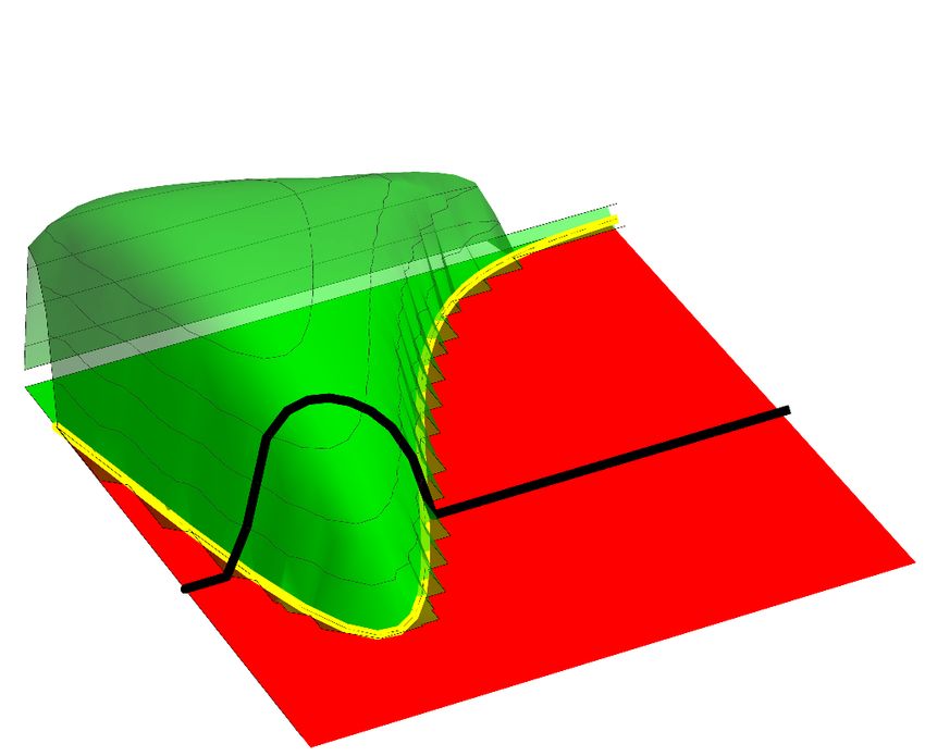
Figure 4: Phase transition in the value of feedback. Left: Optimal control gain varies with channel parameters,
specifically the noise cost for the feedback and feedforward channels. As the feedforward noise cost increases
(black line), the optimal strategy transitions non-monotonically from sending only feedforward messages, to
predictive coding with suppressive feedback, back to sending only feedforward messages, and eventually to
sending no messages. The yellow curve on the panel is the phase transition for feedback: the locus of points
where the optimal strategy is indifferent to sending feedback (green area) or not (red area). Near the critical
point (colored circles), the loss function goes through a phase transition [34], seen at Right: The cost function
has a minimum at Prediction-multiplier D = 0 for low feedforward noise cost, favoring no feedback (red). But
as the feedforward noise cost increases from low to moderate values, this extremum switches to a maximum,
with nearby minima that favor feedback with nonzero D (green). Right at the transition point [34], the system
becomes indifferent to feedback (yellow). Another phase transition occurs in the opposite direction as the
feedforward noise cost increases further from moderate to high values.
For similar reasons, as the world becomes more predictable (Fig 3C), there is a wider range of
feedforward and feedback noise costs for which sending predictions is optimal. The predictability can
be increased either by lengthening the world state timescale, or by enhancing the observation SNR,
enabling better inferences and thereby better predictions. Figs 3D–E demonstrates this for different
world state timescales and measurement gains respectively. However, for large enough feedforward
noise cost, sending even feedforward messages alone becomes too expensive/noisy, and so it is best
to remain silent.
Fig 2A and B show how the optimal control gain L, prediction-multiplier D and observation-multiplier
E change with feedforward noise and feedforward weight respectively. As only the product of noise
variance and weight determines the transition in optimal strategy, we observe the same trend as either
one of them increases. However, these parameters actually exhibit different effects away from the
points of transitions. For example, when feedforward noise is close to 0, the system can save costs by
attentuating the signal (E → 0) and still beat the negligible feedforward noise. In contrast, in the
extreme case that the feedforward messages are nearly free (Wf → 0), the observation-multiplier
increases arbitrarily (E → ∞) to dominate any feedforward noise, improving the inference at no cost.
These limiting cases provide helpful intuitions. Naturally, the challenging regime is in the middle,
where there are real tradeoffs to make, and where feedback becomes relevant.
For the limiting case where feedback noise cost is extremely high, the feedback channel is too
expensive/noisy to be used. Hence, as we slowly increase the feedforward noise cost from zero, we
start by sending just the feedforward messages until the feedforward channel is too expensive/noisy,
at which point we no longer send any messages.
Feedback parameters: We first consider the interesting case of low to moderate feedfoward noise
cost. For low values of feedback noise cost we are in the regime where feedback is cheap and/or
noiseless, and hence it is beneficial to send both predictive feedback and feedforward residual
messages. But when the feedback noise cost becomes too high, sending predictions become too
expensive/noisy, so it is best send only feedforward messages. This is shown in Fig 2C, D. Analogous
to the feedforward case, although the same transition in optimal strategy is observed as we increase
either the feedback noise or feedback weight, these parameters actually exhibit different effects away
from that transition. For example, L → 0 when feedback noise is close to 0, and L → −∞ when
feedback weight is close to 0.
In the case of extremely high feedfoward noise cost, it is not worth sending even an infinitesimal
feedforward message, so the optimal strategy is to not send any messages.
7Sensory parameters: Fig 3C shows the boundary between strategies for three systems with different
levels of predictability. For a fixed value of feedback and feedforward noise costs (dot), the optimal
strategy changes with the predictability. With unpredictable dynamics (thick curve), the dot lies in the
region where sending no messages is optimal, since the feedforward channel is relatively poor (right
of the thick dashed line). For a slightly higher predictability, the dot lies within the region where
feedforward-only messages are optimal (above medium curve, but left of the corresponding dashed
line). And for even higher predictability, the dot lies in the region where predictive coding is optimal
(below the thin curve). Hence, as the predictability increases, there is a transition from sending no
messages, to sending just feedforward messages, to sending both feedback and feedforward messages.
Similarly, if either the measurement gain or the process noise increases, this would yield a higher
observation SNR, which would then improve the inference and thereby predictability. Fig 2E–F
shows the resultant transitions from no messages, to feedforward-only messages, then to predictive
feedback, with increasing measurement gain or process noise. Increasing observation noise has the
opposite effect, making observations less reliable and thereby reducing the predictability. Fig 2G
shows the transitions in strategy with increasing observation noise. Finally, increasing the world
state timescale increases the predictability since it increases both the memory of the system, and the
observation SNR. Fig 2H reveals the familiar sequence of transitions in strategy, supporting our core
intuitions about when feedback is valuable.
6 Discussion
In this paper, we define a new class of dynamic optimization tasks that more accurately capture
essential biological constraints on inference in the brain, by including cost and noise for each
recurrently connected computational element. We solve this optimization problem by modeling
inference as a control problem with prediction as self-control. The resultant optimization provides
nontrivial predictions for when we expect suppressive feedback as a function of biological constraints,
computational costs, and world dynamics.
Predictive coding is a promising theory for brain computations [35–39], and a variety of experimental
studies have indeed shown predictive suppression effects in neural responses [40–47]. However,
neural responses vary in how much they are suppressed depending on a context and signal to noise
ratio. Variants aiming to explain these effects all neglect the computational costs associated with
predictive coding, even though those costs were part of the motivation for saving metabolic costs in
the first place.
Although we contend that it is costly to send predictions, if
these predictions are based on inferences that are already being 0.8 SNR
)
o
C A
D L
computed for a task, then is it really an extra cost to send
Suppression Ratio ( E
them as predictions? Yes, because distinct neurons are used
to send feedforward and feedback signals, so the brain might
pay costs twice for the same inference. When beneficial, the
brain could avoid the duplicate feedback costs by silencing the
feedback neurons, and send its inferences to higher brain areas 0
only through its feedforward neurons. A related question arises World State Timescale
for feedback suppression, which is presumably implemented Figure 5: Example of an experiment
through inhibitory neurons. What is the benefit of turning to validate our theory. Our predictions
on an inhibitory neuron just in order to turn off an excitatory for predictive response suppression as
neuron? Excitatory neurons outnumber inhibitory neurons by as function of world state timescale and
4:1, so few inhibitory neurons can suppress many excitatory observation SNR (decreasing with line
ones, amounting to a potentially substantial savings. These thickness).
biological constraints could be used in future elaborations of computationally constrained inference
models.
One core prediction is that predictive coding grows more favorable when feedforward noise cost is
greater than feedback noise cost. Why would such an asymmetry exist? Biologically, asymmetries
in these noise costs can arise from differences in feedforward and feedback anatomy or functional
properties. Anatomically, feedback projections generally outnumber feedforward ones by 2:1, but the
feedforward pathways compensate with greater weight, dominating at short cortical distances and
leveling off at longer distances [48]. Functionally, the sparser, stronger feedforward channels therefore
8have less ability to average away the noise, leading to a relatively higher amount of metabolically
expensive activity caused by noise, and thus to a higher noise cost. This could establish conditions
under which predictive feedback is useful.
Our mathematical system’s crucial theoretical parameters relate to biological quantities in three ways:
as context-dependent parameters (time constant of the stimulus dynamics, sensory SNR), as neural
parameters that could potentially be manipulated experimentally (feedforward and feedback SNR),
and as developmentally-fixed parameters of the system (feedforward and feedback architecture).
Testing our predicted dependence on these three types of parameters requires different considerations.
The context-dependent parameters are by far the easiest to manipulate experimentally. One can
control the stimulus to adjust the observations’ SNR and the world state timescale, and measure
whether any response suppression is modulated by these controlled parameters as shown in Fig 5.
The internal computational parameters like neural noise may be controllable through stimulus changes
or experimental techniques of causal manipulation. Electrical or optogenetic stimulation could directly
inject neural variability. Another approach could be based on the fact that neural noise variance
tends to increase with firing rate. Thus, one could test our predictions about computational noise
by elevating firing rates. Such methods could include providing a background sensory stimulus, or
direct neural stimulation to increase baseline activity. In any case, it would be important to apply
either natural manipulations or chronic unnatural ones to give the brain enough time and experience
to optimize its computations.
For the developmentally fixed parameters like architecture, we cannot easily alter the system experi-
mentally, and it may be unreasonable to assume that properties in a real biological system can be
unambiguously mapped to any particular value in our abstract theoretical system. However, we can
compare between brain systems or species with architectural difference, and test whether functional
properties covary with those differences as predicted by our theory. Thus it may be fruitful to compare
between brain areas with different architectures, such as 3-layer paleocortex (e.g. olfactory cortex)
versus 6-layer neocortex (e.g. auditory or visual cortex), or within neocortical areas with different
properties. It may also be fruitful to compare between organisms with different architectures (e.g.
mammals versus reptiles). These architectures have different microcircuits with distinct feedforward
and feedback projection neurons. For example, feedback in different visual and motor cortical
systems tends to target different inhibitory cells [49] which have different noise levels [50, 51]. We
predict that systems with more feedback noise (e.g. SOM versus VIP) would have less predictive
suppression, as observed experimentally [49].
There are several interesting avenues for generalizing our theory. The proposed inference as control
method can be extended to the more general case of observer taking external actions in addition to
the internal predictions, in order to maximize external rewards while minimizing both external action
costs (e.g. movements) and internal computational costs. This could be modeled as a typical LQG
control problem [52] for external variables by including appropriate entries in matrices Q, R, and
Baug in addition to the internal controls we use for predictive coding. Though our results are limited
to just a simple one dimensional linear dynamics with uncorrelated noise, our future work will explore
these computational constraints in more complex multivariate and nonlinear tasks. Accounting for
graph-structured inferences [53] and controllability [54] may provide additional constraints on the
brain’s inference processes, and additional predictions for experiments.
Residuals between predictions and observations are useful not just for improving inferences, but
also for learning, which this work does not address. In principle, a multivariate generalization
could explain such computations as hierarchical inferences or adaptation where slower changes are
also subject to prediction. However, the process of learning (as opposed to adaptation) occurs out
of equilibrium with the environment, and accounting for transient responses under nonstationary
statistics will require an extension to our theory. Overall, this work points a way towards expanding
theories of predictive coding and efficient coding to unify inference, learning, and control in biological
systems.
Acknowledgments. The authors thank Itzel Olivos Castillo, Ann Hermundstad, Krešimir Josić,
and Paul Schrater for useful discussions. This work was supported in part by NSF CAREER grant
1552868, the McNair Foundation, and AFOSR grant FA9550-21-1-0422.
9References
[1] Horace B Barlow et al. Possible principles underlying the transformation of sensory messages.
Sensory communication, 1:217–234, 1961.
[2] Rajesh PN Rao and Dana H Ballard. Predictive coding in the visual cortex: a functional
interpretation of some extra-classical receptive-field effects. Nature neuroscience, 2(1):79–87,
1999.
[3] Hilbert J Kappen, Vicenç Gómez, and Manfred Opper. Optimal control as a graphical model
inference problem. Machine learning, 87(2):159–182, 2012.
[4] Hermann Von Helmholtz. Handbuch der physiologischen Optik: mit 213 in den Text einge-
druckten Holzschnitten und 11 Tafeln, volume 9. Voss, 1867.
[5] David C Knill and Alexandre Pouget. The bayesian brain: the role of uncertainty in neural
coding and computation. TRENDS in Neurosciences, 27(12):712–719, 2004.
[6] Wei Ji Ma and Mehrdad Jazayeri. Neural coding of uncertainty and probability. Annual review
of neuroscience, 37:205–220, 2014.
[7] Wei Ji Ma, Jeffrey M Beck, and Alexandre Pouget. Spiking networks for bayesian inference
and choice. Current opinion in neurobiology, 18(2):217–222, 2008.
[8] Stephen W Kuffler. Discharge patterns and functional organization of mammalian retina.
Journal of neurophysiology, 16(1):37–68, 1953.
[9] Haldan Keffer Hartline. The response of single optic nerve fibers of the vertebrate eye to
illumination of the retina. American Journal of Physiology-Legacy Content, 121(2):400–415,
1938.
[10] Peter Kok, Janneke FM Jehee, and Floris P De Lange. Less is more: expectation sharpens
representations in the primary visual cortex. Neuron, 75(2):265–270, 2012.
[11] Christopher Summerfield and Floris P De Lange. Expectation in perceptual decision making:
neural and computational mechanisms. Nature Reviews Neuroscience, 15(11):745–756, 2014.
[12] J Hans van Hateren. Real and optimal neural images in early vision. Nature, 360(6399):68–70,
1992.
[13] Joseph J Atick and A Norman Redlich. Towards a theory of early visual processing. Neural
computation, 2(3):308–320, 1990.
[14] Simon Laughlin. A simple coding procedure enhances a neuron’s information capacity.
Zeitschrift für Naturforschung c, 36(9-10):910–912, 1981.
[15] Mandyam Veerambudi Srinivasan, Simon Barry Laughlin, and Andreas Dubs. Predictive coding:
a fresh view of inhibition in the retina. Proceedings of the Royal Society of London. Series B.
Biological Sciences, 216(1205):427–459, 1982.
[16] Michael W Spratling. Predictive coding as a model of response properties in cortical area v1.
Journal of neuroscience, 30(9):3531–3543, 2010.
[17] Andre M Bastos, W Martin Usrey, Rick A Adams, George R Mangun, Pascal Fries, and Karl J
Friston. Canonical microcircuits for predictive coding. Neuron, 76(4):695–711, 2012.
[18] Matthew Chalk, Olivier Marre, and Gašper Tkačik. Toward a unified theory of efficient,
predictive, and sparse coding. Proceedings of the National Academy of Sciences, 115(1):186–
191, 2018.
[19] Karl Friston and Stefan Kiebel. Predictive coding under the free-energy principle. Philosophical
Transactions of the Royal Society B: Biological Sciences, 364(1521):1211–1221, 2009.
[20] Karl Friston. The free-energy principle: a unified brain theory? Nature reviews neuroscience,
11(2):127–138, 2010.
10[21] Yanping Huang and Rajesh PN Rao. Predictive coding. Wiley Interdisciplinary Reviews:
Cognitive Science, 2(5):580–593, 2011.
[22] Robert Rosenbaum. On the relationship between predictive coding and backpropagation. arXiv
preprint arXiv:2106.13082, 2021.
[23] Haiguang Wen, Kuan Han, Junxing Shi, Yizhen Zhang, Eugenio Culurciello, and Zhongming
Liu. Deep predictive coding network for object recognition. In International Conference on
Machine Learning, pages 5266–5275. PMLR, 2018.
[24] William Lotter, Gabriel Kreiman, and David Cox. Deep predictive coding networks for video
prediction and unsupervised learning. arXiv preprint arXiv:1605.08104, 2016.
[25] Abdullahi Ali, Nasir Ahmad, Elgar de Groot, Marcel AJ van Gerven, and Tim C Kietzmann.
Predictive coding is a consequence of energy efficiency in recurrent neural networks. bioRxiv,
2021.
[26] Kuan Han, Haiguang Wen, Yizhen Zhang, Di Fu, Eugenio Culurciello, and Zhongming Liu.
Deep predictive coding network with local recurrent processing for object recognition. arXiv
preprint arXiv:1805.07526, 2018.
[27] Michael W Spratling. A hierarchical predictive coding model of object recognition in natural
images. Cognitive computation, 9(2):151–167, 2017.
[28] Michael W Spratling. A review of predictive coding algorithms. Brain and cognition, 112:92–97,
2017.
[29] Rakesh Chalasani and Jose C Principe. Deep predictive coding networks. arXiv preprint
arXiv:1301.3541, 2013.
[30] Il Memming Park and Jonathan W Pillow. Bayesian efficient coding. BioRxiv, page 178418,
2017.
[31] Wiktor F Młynarski and Ann M Hermundstad. Adaptive coding for dynamic sensory inference.
Elife, 7:e32055, 2018.
[32] Laurence Aitchison and Máté Lengyel. With or without you: predictive coding and bayesian
inference in the brain. Current opinion in neurobiology, 46:219–227, 2017.
[33] Mark Davis. Stochastic modelling and control. Springer Science & Business Media, 2013.
[34] Lev Davidovich Landau and Evgenii Mikhailovich Lifshitz. Course of theoretical physics.
Elsevier, 2013.
[35] Karl Friston. Does predictive coding have a future? Nature neuroscience, 21(8):1019–1021,
2018.
[36] Xiao Liu, Xiaolong Zou, Zilong Ji, Gengshuo Tian, Yuanyuan Mi, Tiejun Huang, Michael
Kwok Yee Wong, and Si Wu. Push-pull feedback implements hierarchical information retrieval
efficiently. 2019.
[37] Janneke FM Jehee, Constantin Rothkopf, Jeffrey M Beck, and Dana H Ballard. Learning
receptive fields using predictive feedback. Journal of Physiology-Paris, 100(1-3):125–132,
2006.
[38] Samuel J Gershman. What does the free energy principle tell us about the brain? arXiv preprint
arXiv:1901.07945, 2019.
[39] Andreja Bubic, D Yves Von Cramon, and Ricarda I Schubotz. Prediction, cognition and the
brain. Frontiers in human neuroscience, 4:25, 2010.
[40] Toshihiko Hosoya, Stephen A Baccus, and Markus Meister. Dynamic predictive coding by the
retina. Nature, 436(7047):71–77, 2005.
11[41] Jan Homann, Sue Ann Koay, Alistair M Glidden, David W Tank, and Michael J Berry. Predictive
coding of novel versus familiar stimuli in the primary visual cortex. BioRxiv, page 197608,
2017.
[42] Scott O Murray, Daniel Kersten, Bruno A Olshausen, Paul Schrater, and David L Woods.
Shape perception reduces activity in human primary visual cortex. Proceedings of the National
Academy of Sciences, 99(23):15164–15169, 2002.
[43] Ryszard Auksztulewicz and Karl Friston. Repetition suppression and its contextual determinants
in predictive coding. cortex, 80:125–140, 2016.
[44] Tai Sing Lee and David Mumford. Hierarchical bayesian inference in the visual cortex. JOSA
A, 20(7):1434–1448, 2003.
[45] Rajesh PN Rao and Dana H Ballard. Dynamic model of visual recognition predicts neural
response properties in the visual cortex. Neural computation, 9(4):721–763, 1997.
[46] David Mumford. On the computational architecture of the neocortex. Biological cybernetics,
66(3):241–251, 1992.
[47] Marta I Garrido, James M Kilner, Klaas E Stephan, and Karl J Friston. The mismatch negativity:
a review of underlying mechanisms. Clinical neurophysiology, 120(3):453–463, 2009.
[48] Nikola T Markov, Julien Vezoli, Pascal Chameau, Arnaud Falchier, René Quilodran, Cyril
Huissoud, Camille Lamy, Pierre Misery, Pascale Giroud, Shimon Ullman, et al. Anatomy
of hierarchy: feedforward and feedback pathways in macaque visual cortex. Journal of
Comparative Neurology, 522(1):225–259, 2014.
[49] Shan Shen, Xiaolong Jiang, Federico Scala, Jiakun Fu, Paul Fahey, Dimitry Kobak, Zhenghuan
Tan, Jacob Reimer, Fabian Sinz, and Andreas S Tolias. Distinct organization of two cortico-
cortical feedback pathways. bioRxiv, 2020.
[50] Wen-pei Ma, Bao-hua Liu, Ya-tang Li, Z Josh Huang, Li I Zhang, and Huizhong W Tao.
Visual representations by cortical somatostatin inhibitory neurons—selective but with weak and
delayed responses. Journal of Neuroscience, 30(43):14371–14379, 2010.
[51] Daniel J Millman, Gabriel Koch Ocker, Shiella Caldejon, Josh D Larkin, Eric Kenji Lee, Jennifer
Luviano, Chelsea Nayan, Thuyanh V Nguyen, Kat North, Sam Seid, et al. Vip interneurons in
mouse primary visual cortex selectively enhance responses to weak but specific stimuli. Elife,
9:e55130, 2020.
[52] Rudolf Emil Kalman et al. Contributions to the theory of optimal control. Bol. soc. mat.
mexicana, 5(2):102–119, 1960.
[53] Xaq Pitkow and Dora E Angelaki. Inference in the brain: statistics flowing in redundant
population codes. Neuron, 94(5):943–953, 2017.
[54] Shi Gu, Fabio Pasqualetti, Matthew Cieslak, Qawi K Telesford, B Yu Alfred, Ari E Kahn,
John D Medaglia, Jean M Vettel, Michael B Miller, Scott T Grafton, et al. Controllability of
structural brain networks. Nature communications, 6(1):1–10, 2015.
12A Appendix
A.1 Shoehorning the inference tracking dynamics as an LQG control problem
Substituting Eqs 1- 2, and 4-5 in Eq 6.
˜ t =∆t + ηft
∆
=(D p̃t + E ot ) + ηft
=D p̃t + E (C xt + ηot ) + ηft
=D p̃t + E C xt + E ηot + ηft
=D p̃t + E C (A xt−1 + ηpt ) + E ηot + ηft
=D p̃t + E C A xt−1 + E C ηpt + E ηot + ηft
=D (pt + ηbt ) + E C A xt−1 + E C ηpt + E ηot + ηft
=E C A xt−1 + D pt + E C ηpt + E ηot + D ηbt + ηft (15)
>
˜ t as in Eq 16.
Combining Eqs 1 and 15, we write the dynamics of augmented state z t = xt ∆
The noisy residual can now be written as a partial observation of the augmented state (Eq 17).
t−1
ηaug
Aaug t−1 Baug z }| {
z t
t
z }| {
z }| { z}|{ ηpt
0 xt−1
x A 0 t I 0 0 0 ηo
zt = ˜ t = ˜ t−1 + D p + E C (16)
∆ ECA 0 ∆ E D I ηbt
ηft
t
˜ t x
∆ = [0 I] ˜ t (17)
| {z } ∆
Caug | {z }
zt
Rewriting Eqs 16-17 using concise notation, we get the LQG dynamics equations where prediction p
is treated as the control.
z t =Aaug z t−1 + Baug pt + ηaug
t−1
˜ t =Caug z t
∆
A.2 Feedforward and feedback energy costs expressed as the LQG state and control costs
respectively
We express the feedforward and feedback energy costs as the LQG
state and control costs respectively.
0 0
For the derivation, we introduce the matrices Q = , and R = Wb . We take the feedback
0 Wf
noise ηb as i.i.d ∼ N (0, Σb ) .
T T
1 X ˜ t> ˜ t + p̃t > Wb p̃t = min lim 1
X
˜ t > Wf ∆
˜ t + (pt + η t )> Wb (pt + η t )
min lim ∆ Wf ∆ ∆ b b
p T →∞ T p T →∞ T
t=1 t=1
T
1 X ˜ t> ˜ t + pt > Wb pt + η t > Wb ηbt
= min lim ∆ Wf ∆ b
p T →∞ T
t=1
T
1 X ˜ t>
˜ t + pt > Wb pt + T r(Wb Σb )
= min lim ∆ Wf ∆
p T →∞ T
t=1
T
1 X t> >
= min lim z Q z t + pt R pt + T r(Wb Σb )
p T →∞ T
t=1
T
1 X t> >
= min lim z Q z t + pt R pt
p T →∞ T | {z } | {z }
t=1 state cost control cost
13A.3 Minimizing the total energy cost also minimizes the inference cost, for a fixed D& E
The LQG problem of interest is described by Eqs 10–12. The separation principle states that the
solution for LQG problem includes an estimation part and a control part, both of which jointly form
the optimal solution even if treated separately. The estimation part of LQG solution minimizes the
average squared norm error between estimated state ẑ and the true state z, as shown in the left side of
equality in Eq 18. Note that at any time t, we get to observe all the evidence up until that time (i.e
∆˜ 1, ∆
˜ 2 ,.., ∆
˜ t ). This enables the simplification from Eq 18 to 19, because the optimal estimate ∆ˆ˜ t
given ∆˜t is trivially ∆ ˜ t itself. Hence, from Eq 20, we conclude that although we define the LQG
objective function to be just the total energy cost, the LQG solution that minimizes the total energy
cost also minimizes the inference cost for a fixed D and E.
T T t t
1X t t > t t 1 X xt x̂ > xt x̂
lim (z − ẑ ) (z − ẑ ) = lim ( ˜ t − ˆ˜ t ) ( ˜ t − ˆ˜ t ) (18)
T →∞ T T →∞ T ∆ ∆ ∆ ∆
t=1 t=1
T
1X t
= lim (x − x̂t )> (xt − x̂t ) (19)
T →∞ T
t=1
=Costinf (20)
A.4 LQG estimation solution to find F , G, and H in terms of D and E
The optimal estimate of the augmented state based on its noisy partial observations is given as
˜ t + (I − K Caug )Baug pt
ẑ t =(I − K Caug )Aaug ẑ t−1 + K ∆ (21)
T > −1
K =Σ̌ Caug (Caug Σ̌ Caug ) ,
where Σ̌ is the solution to a discrete algebraic Riccati equation (Eq 22), with W as the covariance of
noise vector ηaug .
Σ̌ = Aaug Σ̌ A> > > −1
aug + W − Aaug Σ̌ Caug (Caug Σ̌ Caug ) Caug Σ̌ A>
aug (22)
For brevity, we rewrite Eq 21 in terms of block matrics using the following substitutions,
Faug =(I − K Caug )Aaug , Haug = (I − K Caug )Baug
t
(Faug )11 (Faug )12 x̂t−1
x̂ (K)1 ˜ t (Haug )1 t
∆˜ t = (Faug )21 (Faug )22 ∆ ˜ t−1 + (K)2 ∆ + (Haug )2 p (23)
yielding
˜ t−1 + (K)1 ∆
x̂t =(Faug )11 x̂t−1 + (Faug )12 ∆ ˜ t + (Haug )1 pt (24)
˜ t =(Faug )21 x̂t−1 + (Faug )22 ∆
∆ ˜ t−1 + (K)2 ∆
˜ t + (Haug )2 pt .
Since the states are Markovian, consequently the optimal estimates are Markovian as well. This
˜ t−1 . Likewise, ∆
implies that x̂t given x̂t−1 , does not depend on ∆ ˜ t given ∆
˜ t , does not depend on
t−1 ˜ t−1 t
x̂ , ∆ , and p . The above two arguments can be used to deduce that
(Faug )12 = 0, (Faug )21 = 0, (Faug )22 = 0 (K)2 = I, (Haug )2 = 0.
which we also verified empirically for the one dimensional case. Substituting (Faug )12 = 0 in Eq 24
and comparing it with Eq 7, we get the optimal solutions for F , G, and H in terms of D and E,
denoted as F 0 , G0 , and H 0 respectively.
F 0 = (Faug )11 , G0 = (K)1 , H 0 = (Haug )1
A.5 LQG control solution to find L in terms of D and E
The optimal LQG control is given as
pt =Laug ẑ t−1 (25)
>
Laug = − (R + Baug P Baug )−1 Baug
>
P Aaug (26)
14where P is the solution of a discrete algebraic Riccati equation (Eq 27).
P = Q + A> > >
aug P Aaug − Aaug P Baug (R + Baug P Baug )
−1 >
Baug P Aaug (27)
As shown in Eq 16, the last set of columns in Aaug are all zero vectors. As a consequence, since
Aaug is the last multiplier in the right side of equality in Eq 25, the last set of columns of Laug would
also be zero vectors. More specifically, Eq 25 can be further simplified by writing Laug in terms of
block matrices in the following way
t−1
x̂ ˜ t−1 , then (Laug )2 = 0
p = [(Laug )1 (Laug )2 ] ˜ t−1 =(Laug )1 x̂t−1 + (Laug )2 ∆
t
∆
=⇒ pt =(Laug )1 x̂t−1
Hence, the optimal prediction is linearly related to the estimate through (Laug )1 . For consistency in
notations, we denote (Laug )1 as L0 , yielding
pt = L0 x̂t−1 , where L0 = (Laug )1 .
A.6 Closed form expressions for total cost in terms of D and E
The optimal inference cost for fixed D and E, which is the same as the augmented state’s estimation
error, is Cost0inf = T r(Σ). Where Σ is the augmented state’s estimation error covariance matrix,
such that
> > −1
Σ = Σ̌ − Σ̌ Caug (Caug Σ̌ Caug ) Caug Σ̌. (28)
The optimal total energy cost for a given D and E, which is the optimal LQG cost, is given as
Cost0energy = T r(Q Σ) + T r(P (Σ̌ − Σ)). As Σ is the error covariance matrix in estimating z t ,
˜ t is fully observable at any time point, the corresponding lower block
and since the noisy residual ∆
matrix in Σ will be zero. Also, by definition in Eq 12, we know that the upper block matrix in Q is
zero. As a consequence, T r(Q Σ) would always be zero. Resulting in Cost0energy = T r(P (Σ̌ − Σ)).
Combining the inference cost and energy cost, we have the total cost in terms of D and E as
Cost0tot = T r(Σ) + T r(P (Σ̌ − Σ)) (29)
A.7 Condition for useful feedback
It can be algebraically shown that the total cost is an even function in both D and E and hence can
be written as a function of Ď = D2 and Ě = E 2 . This limits the function domain to non-negative
values, thereby reducing the search space for numerical optimization. We empirically observe that
the cost function now has just one minimum when plotted with Ď and Ě, and that the negative of
gradient at any point always directs toward this minimum.
Let Ě 0 denote the optimal Ě that minimizes the total cost at Ď = 0. Ě 0 can be computed by equating
the derivative of cost with respect to Ě to 0, at Ď = 0 (Eq 30).
∂Cost0tot
=0 (30)
∂ Ě Ď=0,Ě=Ě 0
We define ψ as the derivative of total cost with respect to Ď, evaluated at Ď = 0 and Ě = Ě 0 (Eq 31).
∂Cost0tot
ψ= (31)
∂ Ď Ď=0,Ě=Ě 0
Since the negative of gradient always points to the minimum, the following holds true: If ψ is
negative, then the negative of gradient points towards non-zero Ď, implying the optimal Ď is non-
zero. However, given that the domain of Ď is non-negative, if ψ is non-negative then the optimal Ď
is 0. Therefore, the optimal Ď is non-zero if and only if ψ < 0. These conditions can be concisely
written as
C2
Ubn < Φ(Ufn , A, σp2 , 2 ). (32)
σo
where Φ is a complicated function involving the roots Ě 0 of the quartic equation Eq 30 substituted
into Eq 31. Ultimately we use these analytic expressions to solve numerically for the remaining
conditions on the optimal prediction-multiplier D and observation-multiplier E.
15You can also read