Photo-astrometric distances, extinctions, and astrophysical - Astronomy & Astrophysics
←
→
Page content transcription
If your browser does not render page correctly, please read the page content below
A&A 658, A91 (2022)
https://doi.org/10.1051/0004-6361/202142369                                                                        Astronomy
c ESO 2022                                                                                                          &
                                                                                                                   Astrophysics

       Photo-astrometric distances, extinctions, and astrophysical
         parameters for Gaia EDR3 stars brighter than G = 18.5?
F. Anders1,2 , A. Khalatyan2 , A. B. A. Queiroz2,3,4 , C. Chiappini2,3 , J. Ardèvol1, L. Casamiquela5 , F. Figueras1,
Ó. Jiménez-Arranz1 , C. Jordi1 , M. Monguió1 , M. Romero-Gómez1 , D. Altamirano1, T. Antoja1 , R. Assaad6 ,
     T. Cantat-Gaudin7 , A. Castro-Ginard8 , H. Enke2 , L. Girardi9 , G. Guiglion2 , S. Khan10 , X. Luri1 ,
             A. Miglio11,12,13 , I. Minchev2 , P. Ramos14 , B. X. Santiago15,3 , and M. Steinmetz2

       1
           Institut de Ciències del Cosmos, Universitat de Barcelona (IEEC-UB), Martí i Franquès 1, 08028 Barcelona, Spain
           e-mail: fanders@icc.ub.edu
       2
           Leibniz-Institut für Astrophysik Potsdam (AIP), An der Sternwarte 16, 14482 Potsdam, Germany
           e-mail: akhalatyan@aip.de
       3
           Laboratório Interinstitucional de e-Astronomia – LIneA, Rua Gal. José Cristino 77, Rio de Janeiro 20921-400, Brazil
       4
           Institut für Physik und Astronomie, Universität Potsdam, Haus 28 Karl-Liebknecht-Str. 24/25, 14476 Golm, Germany
       5
           Laboratoire d’Astrophysique de Bordeaux, Univ. Bordeaux, CNRS, B18N, allée Geoffroy Saint-Hilaire, 33615 Pessac, France
       6
           Department of Physics, University of Surrey, Guildford GU2 7XH, UK
       7
           Max-Planck-Institut für Astronomie, Königstuhl 17, 69117 Heidelberg, Germany
       8
           Leiden Observatory, Leiden University, Niels Bohrweg 2, 2333 CA Leiden, The Netherlands
       9
           Osservatorio Astronomico di Padova, INAF, Vicolo dell’Osservatorio 5, 35122 Padova, Italy
      10
           Institute of Physics, Laboratory of Astrophysics, École Polytechnique Fédérale de Lausanne (EPFL), Observatoire de Sauverny,
           1290 Versoix, Switzerland
      11
           Dipartimento di Fisica e Astronomia, Università di Bologna, Via Gobetti 93/2, 40129 Bologna, Italy
      12
           INAF – Osservatorio di Astrofisica e Scienza dello Spazio di Bologna, Via Gobetti 93/3, 40129 Bologna, Italy
      13
           School of Physics and Astronomy, University of Birmingham, Edgbaston B15 2TT, UK
      14
           Observatoire astronomique de Strasbourg, Université de Strasbourg, CNRS, 11 rue de l’Université, 67000 Strasbourg, France
      15
           Instituto de Física, Universidade Federal do Rio Grande do Sul, Caixa Postal 15051, Porto Alegre 91501-970, Brazil

     Received 4 October 2021 / Accepted 5 November 2021

                                                                 ABSTRACT

     We present a catalogue of 362 million stellar parameters, distances, and extinctions derived from Gaia’s Early Data Release (EDR3)
     cross-matched with the photometric catalogues of Pan-STARRS1, SkyMapper, 2MASS, and AllWISE. The higher precision of the
     Gaia EDR3 data, combined with the broad wavelength coverage of the additional photometric surveys and the new stellar-density
     priors of the StarHorse code, allows us to substantially improve the accuracy and precision over previous photo-astrometric stellar-
     parameter estimates. At magnitude G = 14 (17), our typical precisions amount to 3% (15%) in distance, 0.13 mag (0.15 mag) in
     V-band extinction, and 140 K (180 K) in effective temperature. Our results are validated by comparisons with open clusters, as well as
     with asteroseismic and spectroscopic measurements, indicating systematic errors smaller than the nominal uncertainties for the vast
     majority of objects. We also provide distance- and extinction-corrected colour-magnitude diagrams, extinction maps, and extensive
     stellar density maps that reveal detailed substructures in the Milky Way and beyond. The new density maps now probe a much greater
     volume, extending to regions beyond the Galactic bar and to Local Group galaxies, with a larger total number density. We publish
     our results through an ADQL query interface (gaia.aip.de) as well as via tables containing approximations of the full posterior
     distributions. Our multi-wavelength approach and the deep magnitude limit render our results useful also beyond the next Gaia release,
     DR3.
     Key words. stars: distances – stars: fundamental parameters – Galaxy: general – Galaxy: stellar content – Galaxy: structure

1. Introduction                                                          solar vicinity (e.g. Gaia Collaboration 2021a,b; Reylé et al.
                                                                         2021), open star clusters (e.g. Cantat-Gaudin et al. 2018;
Since its launch in 2013 the European Space Agency’s flag-
                                                                         Cantat-Gaudin & Anders 2020; Castro-Ginard et al. 2020), dis-
ship mission Gaia (Gaia Collaboration 2016) has revolutionised
Galactic astronomy and its neighbouring fields (Brown 2021).             tant regions of the Milky Way (e.g. Ramos et al. 2021;
The precision and accuracy of our knowledge of the Solar Sys-            Gaia Collaboration 2021c; Zari et al. 2021) and the Local Group
tem (e.g. Gaia Collaboration 2018a; Bailer-Jones et al. 2018a;           (e.g. Gaia Collaboration 2018b, 2021d; Antoja et al. 2020), the
Portegies Zwart 2021), stellar astrophysics (e.g. Jao et al. 2018;       Galactic potential (e.g. Crosta et al. 2020; Cunningham et al.
Lanzafame et al. 2019; Mowlavi et al. 2021), the immediate               2020; Hattori et al. 2021), and even the Hubble constant (e.g.
                                                                         Breuval et al. 2020; Riess et al. 2021; Baumgardt & Vasiliev
 ?                                                                       2021) are constantly increasing thanks to Gaia.
   The catalog is available at the CDS via anonymous ftp to
cdsarc.u-strasbg.fr (130.79.128.5) or via http://cdsarc.                     In the context of Galactic archaeology, Gaia has also
u-strasbg.fr/viz-bin/cat/J/A+A/658/A91                                   enabled a completely new line of precision studies tracing

                                                      Article published by EDP Sciences                                        A91, page 1 of 27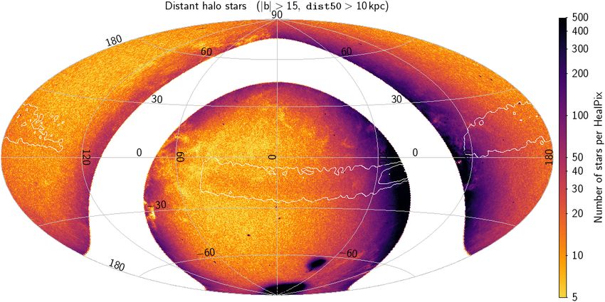
A&A 658, A91 (2022)

the past accretion events of the Milky Way (Helmi 2020;              vious results obtained from Gaia DR2 and EDR3 in Sect. 6.
Kruijssen et al. 2020; Pfeffer et al. 2021). Often this is           Finally, we conclude the paper with a summary and a brief out-
achieved by combining the complete phase-space informa-              look to the near future in Sect. 7.
tion with detailed chemistry from spectroscopic surveys (e.g.
Aguado et al. 2021; Gudin et al. 2021; Limberg et al. 2021a,b;
Montalbán et al. 2021; Naidu et al. 2021; Shank et al. 2021).
     The latest Gaia data release, Early Data Release 3 (Gaia        2. Data
EDR3; Gaia Collaboration 2021e), covers the first 34 months of       As input for StarHorse, we use the Gaia EDR3 data cross-
observations with positions and photometry for 1.8×10⁹ sources       matched with 2MASS, AllWISE, Pan-STARRS1, and SkyMap-
(Riello et al. 2021), proper motions and parallaxes for 1.5 × 10⁹    per (Onken et al. 2019), in the sense that all available good pho-
sources (Lindegren et al. 2021a), and radial velocities for 7 ×      tometric measurements are used in the inference. The calibra-
106 sources (Seabroke et al. 2021; Gaia Collaboration 2021e).        tions used in this paper are summarised in Table 1.
With respect to Data Release 2 (Gaia DR2; Gaia Collaboration             From Gaia EDR3 we use the parallaxes and three-band
2018c), the proper motions are by a factor of 2 more precise, and    photometry, together with their associated uncertainties. We
parallax uncertainties are reduced by 20% (see Fabricius et al.      recalibrate the parallaxes following the recommendations of
2021 for details).                                                   Lindegren et al. (2021b) who assessed the variations in the
     In a previous work (Anders et al. 2019, hereafter A19) based    parallax zero point as a function of sky position, magnitude,
on Gaia DR2, our group derived Bayesian stellar parame-              and colour1 . Furthermore, we inflate the corresponding paral-
ters, distances, and extinctions for 265 million stars brighter      lax uncertainties by a magnitude-dependent factor, following
than G = 18 with the StarHorse code (Santiago et al. 2016;           Fabricius et al. (2021, see also El-Badry et al. 2021). In partic-
Queiroz et al. 2018). The combination of precise Gaia DR2            ular, we fit the inflation factor to their worst-case scenario of
parallaxes and optical photometry with the multi-wavelength          Fig. 19 in Fabricius et al. (2021) (a crowded Large Magellanic
photometry of Pan-STARRS1 (Chambers et al. 2016), 2MASS              Cloud field) to make sure that our parallax uncertainties are not
(Cutri et al. 2003), and AllWISE (Cutri et al. 2013) substantially   underestimated. A further discussion of the fidelity of the Gaia
improved the accuracy of the extinction and effective temper-        parallaxes in our context is available in Rybizki et al. (2022) and
ature estimates provided with only Gaia DR2 (Andrae et al.           in our Sect. 3.3.1.
2018). A selection of the most reliable in- and output data, a           Regarding the Gaia photometry, we use the precise
sample of 137 million stars, allowed A19 to detect the imprint       EDR3 magnitudes (Riello et al. 2021) without any poste-
of the Galactic bar both in the stellar density distribution and     rior correction other than the G-band correction advertised
in proper motion maps (further studied with APOGEE spec-             in Appendix A of Gaia Collaboration (2021e)2 , since they
troscopy in Queiroz et al. 2021).                                    show much lower systematics (.0.01 mag; e.g. Fabricius et al.
     The results of our Gaia DR2 StarHorse run presented in          2021; Niu et al. 2021) than the previous DR2 photometry (see
A19 have been used in a wide variety of science cases, including     e.g. Maíz Apellániz & Weiler 2018). For the BP/RP photome-
exoplanetary research (Sozzetti et al. 2021), interstellar extinc-   try, we follow the recommendation of Fabricius et al. (2021)
tion (Leike et al. 2020), runaway stars from supernova remnants      and do not use magnitudes phot_bp_mean_mag > 20.5 or
(Lux et al. 2021), X-ray transients (Lamer et al. 2021), γ-ray       phot_rp_mean_mag > 20 in the inference.
astronomy (Steppa & Egberts 2020), ,the Galactic escape speed            The Gaia EDR3 cross-match to the large-area photometric
curve (Monari et al. 2018), the three-dimensionl phase-space         surveys 2MASS, AllWISE, Pan-STARRS1 DR1, and SkyMap-
structure of the Milky Way disc (Carrillo et al. 2019), and spec-    per DR2 is documented in Marrese et al. (2021). The main nov-
troscopic survey simulations (Chiappini et al. 2019).                elty with respect to A19 is the inclusion of SkyMapper data.
     Anticipating a significant improvement thanks to the new        From the SkyMapper DR2 data we only use the griz bands
Gaia data, we update our analysis using the new EDR3 data in         (with zero points recalibrated following Huang et al. 2021a) and
this paper, addressing some of the known caveats of our previous     refrain from using the u and v bands, because our default extinc-
data release and reducing the uncertainties of the main output       tion law (Schlafly et al. 2016) should not be extrapolated to the
parameters by a factor of 2. In a parallel effort we will be pub-    ultraviolet.
lishing StarHorse results for spectroscopic surveys combined             For Pan-STARRS1, we apply the zero-point corrections rec-
with Gaia (≈6 million stars) in Queiroz et al. (in prep.).           ommended by Scolnic et al. (2015), and do not use magnitudes
     This paper is structured as follows: Section 2 presents the     brighter than the saturation limit. With respect to A19, we apply
input data and Sect. 3 our method. In particular, Sect. 3.1          more restrictive filters to the 2MASS and AllWISE photometry:
describes the updates to our code with respect to previous           only magnitudes with corresponding photometric quality flags
applications, and Sect. 3.3 explains how we flagged the new          ‘A’ or ‘B’ are accepted. The minimum photometric uncertainties
StarHorse results for Gaia EDR3. We then present some                used in the inference (reflecting also the systematic uncertainties
first astrophysical results in Sect. 4, mainly focussing on          of the passbands and the bolometric corrections) are given in
colour-magnitude diagrams (CMDs), extinction maps, and stel-         Table 1. We also note that for .0.5% of the Gaia EDR3 sources,
lar density maps. The stellar density maps demonstrate the           the Gaia cross-match with 2MASS returns in multiple matches.
emergence of substructure beyond the detection of the Galac-         In these cases (pointing towards possible confusion), we do not
tic bar, for example when focussing on metal-poor stars, the         use any 2MASS photometry.
Magellanic Clouds, or the outer Milky Way halo. The pre-
cision and accuracy of the StarHorse EDR3 parameters are
discussed in Sect. 5, providing comparisons to Galactic open         1
                                                                       Code available at https://gitlab.com/icc-ub/public/
clusters (OCs Cantat-Gaudin et al. 2020; Dias et al. 2021), aster-   gaiadr3_zeropoint/-/tree/master/
oseismically derived parameters for giant stars (Miglio et al.       2
                                                                       https://github.com/agabrown/
2021), and spectroscopic stellar parameters from the GALAH           gaiaedr3-6p-gband-correction/blob/main/
survey (Buder et al. 2021). We also make comparisons to pre-         GCorrectionCode.ipynb

A91, page 2 of 27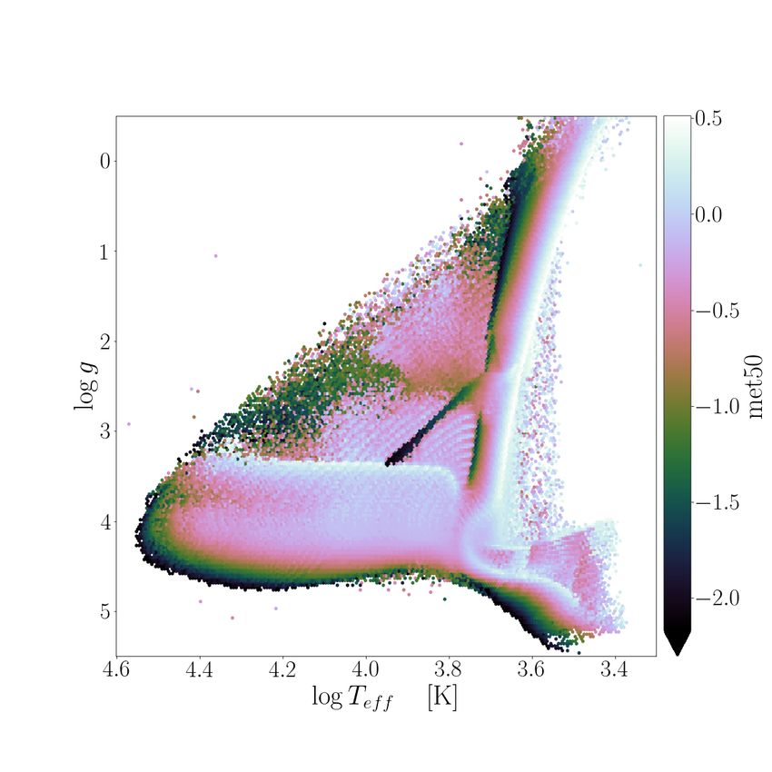
F. Anders et al.: StarHorse parameters for Gaia EDR3 stars

Table 1. Summary of the calibrations and data curation applied to the astrometric and photometric data for this work.

           Parameter             Parameter regime            Calibration choice                     Reference
           $cal                                              Use zpt.py calibration                 Lindegren et al. (2021b)
           σcal
             $                                               uwu(G) · parallax_error                Fit to Fabricius et al. (2021) Fig. 19a&b
           G            astrometric_params_solved = 95       Colour-dependent correction            Gaia Collaboration (2021e) Appendix A
           gPS1               g_mean_psf_mag > 14            g_mean_psf_mag − 0.020
           rPS1               r_mean_psf_mag > 15            r_mean_psf_mag − 0.033
           iPS1               i_mean_psf_mag > 15            i_mean_psf_mag − 0.024                 Scolnic et al. (2015)
           zPS1               z_mean_psf_mag > 14            z_mean_psf_mag − 0.028
           yPS1               y_mean_psf_mag > 13            y_mean_psf_mag − 0.011
           gSM , rSM                                         E(B − V) dependent zero-point shifts   Huang et al. (2021a)
           uSM , vSM                                         Not used in inference                  Schlafly et al. (2016)
           σmag                    Gaia EDR3                 max{σmag,source , 0.02mag}
                                2MASS, AllWISE               max{σmag,source , 0.03 mag}
                               Pan-STARRS1 DR1               max{σmag,source , 0.04 mag}
                                 SkyMapper DR2               max{σmag,source , 0.05 mag}

3. Method: The StarHorse code                                              10 mag, considering that our sample is limited by G < 18.5). The
                                                                           extinction prior is then defined as a very broad Gaussian distri-
StarHorse (Queiroz et al. 2018) is an isochrone-fitting code tai-          bution around the central value (with σAV,prior = max{0.2, 0.33 ·
lored to derive distances d, extinctions (at λ = 542 nm) AV , ages         AVprior }).
τ, masses m∗ , effective temperatures T eff , metallicities [M/H],
and surface gravities log g for field stars. In the absence of spec-
troscopic input data, it takes as input only the measured parallax         3.1.2. Extragalactic priors
$ and a set of observed magnitudes mλ to estimate how close a
stellar model is to the observed data.                                     In A19 we saw that the stellar populations of the Magellanic
     StarHorse also includes priors about the geometry, metal-             Clouds, the Sagittarius (Sgr dSph) galaxy, and a number of rel-
licity and age characteristics of the main Galactic components.            atively nearby globular clusters, whose stellar densities were
The priors adopted here are very similar to those in Queiroz et al.        not accounted for by our priors until now, left a spurious
(2018), A19, and Queiroz et al. (2020): a Chabrier (2003) ini-             imprint on the posterior Galactic density distribution inferred
tial mass function; exponential spatial density profiles for thin          with StarHorse.
and thick discs; a spherical halo and a triaxial bulge/bar com-                 For the new runs we therefore included new extragalactic and
ponent, as well as broad Gaussian distributions for the age and            globular cluster priors in the calculation of the global prior. For
metallicity distribution priors. The normalisation of each Galac-          the extragalactic resolved stellar population we use the updated
tic component, as well as the solar position, were taken from              list (October 2019) of Local Group Galaxies from McConnachie
Bland-Hawthorn & Gerhard (2016).                                           (2012), which comprises sky positions, distances, foreground
                                                                           extinctions, apparent dimensions, central densities, metallicities,
                                                                           masses, and other basic quantities for the Local Group. We man-
3.1. Code updates and improvements                                         ually added M31 to this list, and curated the list for the most
                                                                           prominent objects on the sky: the Magellanic Clouds and the
With respect to A19 and Queiroz et al. (2020), we have imple-              Sgr dSph galaxy. For all but these objects we estimate the mass
mented some changes that help to improve the performance of                of the external galaxy by inverting the mass-metallicity relation
StarHorse in the context of Gaia EDR3.                                     of Panter et al. (2008) (linearly extrapolated below [Fe/H] = −1).
                                                                           For the Galactic globular clusters we used the recent catalogue
3.1.1. A more informative interstellar extinction prior                    of Hilker et al. (2020).
One of the drawbacks of the A19 Gaia DR2 run was the                            The sky distribution of all considered objects is shown in
a priori limit in interstellar extinction to AV < 4 mag                    Fig. 1. If a star’s celestial coordinates coincide with those of an
for sources with low signal-to-noise parallax measurements                 external galaxy or globular cluster within five half-light radii, we
(parallax_over_error < 5). This resulted in poor conver-                   add to the Milky Way foreground prior an additional population
gence or biased results for distant obscured objects in the                corresponding to the characteristics of that object (stellar den-
Galactic plane. For the present EDR3 run we therefore update               sity, distance, metallicity). For the sake of simplicity, the density
our previously uninformative top-hat AV prior to a prior                   profile priors for all objects are assumed to be three-dimensional
that takes into account our knowledge of Galactic interstellar             Gaussians.
extinction.
    For the region of the sky covered by Pan-STARRS1, we use               3.1.3. Update of the bar angle in the priors
the large-scale three-dimensional extinction map of Green et al.
(2019). For the missing part (1/4) of the sky, we use the 2MASS-           Our knowledge about the large-scale parameters of the Milky
derived three-dimensional extinction model by Drimmel et al.               Way is constantly improving. In light of the growing evi-
(2003). To get the range of possible distances for each star               dence for a bar angle around 27 ± 2 deg (see discus-
(needed to query the extinction maps), we invert the EDR3                  sion in Bland-Hawthorn & Gerhard 2016, reinforced also by
zero-point-corrected parallax measurements to estimate a prior             Queiroz et al. 2021), we have updated the angle of the Galactic
extinction value range for each star (using a maximum of AVprior =         bar in our prior to that value.

                                                                                                                                     A91, page 3 of 27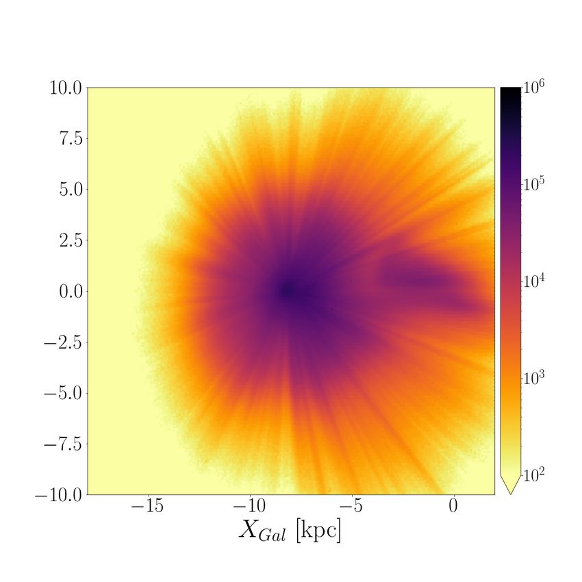
A&A 658, A91 (2022)

Fig. 1. Newly implemented priors in the StarHorse code. Top panel: sky distribution (in Galactic coordinates) of extragalactic and globular-
cluster priors added in the new StarHorse version. The angular extents (5 effective radii) of each of the Local Group priors are shown as circles,
highlighting the most prominent objects: the Magellanic Clouds, the Sgr dSph, and Andromeda. Bottom panel: median prior V-band extinction
per HealPix. The extinction prior is calculated individually for each star from the three-dimensional extinction maps of either Green et al. (2019)
or Drimmel et al. (2003).

3.1.4. Taking into account evolution of surface metallicity                rarer) than main sequence stars, especially in nearby volume-
                                                                           limited samples.
We adopt here the latest version of the PARSEC1.2S + COL-
IBRI S37 stellar evolutionary model tracks (Bressan et al. 2012;
Marigo et al. 2017; Pastorelli et al. 2019). Using these tracks in         3.2. StarHorse setup
conjunction with the new CMD web interface allows us to take               For the EDR3 run we used a grid of PARSEC 1.2S stellar models
into account changes in the surface metallicity of stars during            (Marigo et al. 2017) in the 2MASS, Pan-STARRS1, SkyMap-
stellar evolution. While the effect is typically very small, element       per, Gaia EDR3, and WISE photometric systems available on
diffusion does introduce some small but appreciable decrease               the PARSEC web page3 . The model grid was equally spaced by
in the surface metal content for solar-mass stars before and               0.1 dex in log age as well as in initial metallicity [M/H]. The code
around the turn-off (Fig. 2; see e.g. Bertelli Motta et al. 2018;          explores distances within {1/($cal + 3 · σcal          cal
                                                                                                                                      − 3 · σcal
                                                                                                                        $ ), 1/($            $ )}.
Souto et al. 2019 for observational evidence). The effect is much              For the present Gaia EDR3 run (G < 18.5 mag, 400M stars),
stronger for low-metallicity stars. The opposite (i.e. a strong            the code took on average 0.3 s per star to run (depending slightly
increase in the surface metallicity) happens for a fraction of             on the position in the CMD and the number of photometric mea-
the more evolved stars, such as those in the thermally puls-               surements available). In total, the computational cost for this
ing asymptotic giant branch and Wolf-Rayet phases; this lat-
ter effect, however, is much less relevant to our results given            3
                                                                             http://stev.oapd.inaf.it/cgi-bin/cmd_3.4;                 see    also
that these evolutionary phases are much shorter-lived (and hence           http://stev.oapd.inaf.it/cmd_3.4/faq.html

A91, page 4 of 27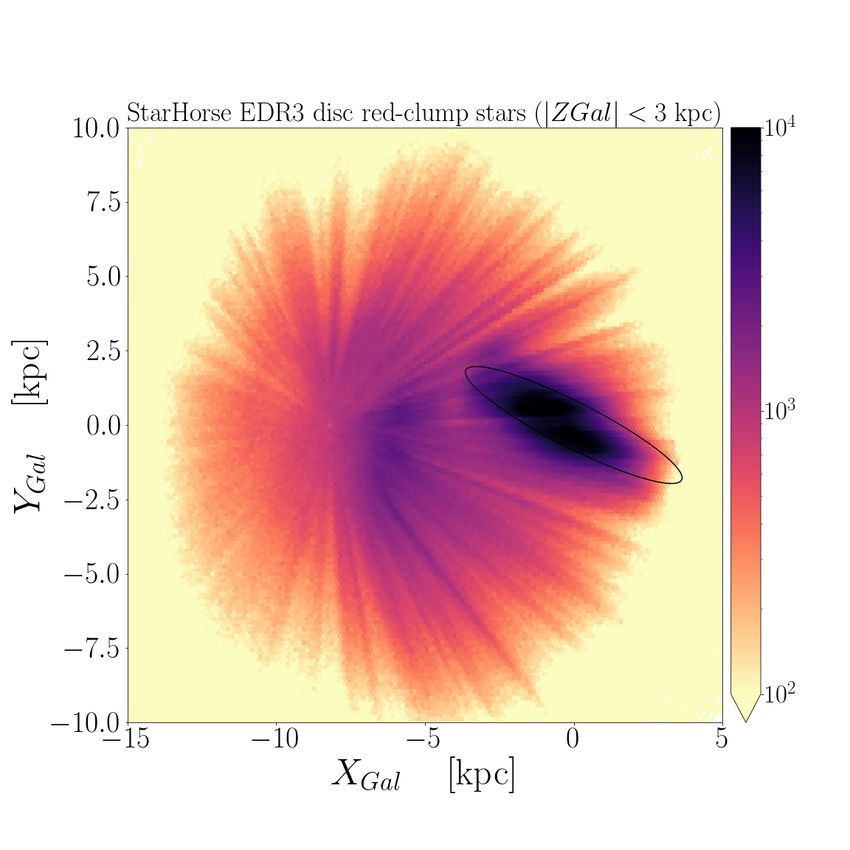
F. Anders et al.: StarHorse parameters for Gaia EDR3 stars

                                                                            on the DR2 recommendations by the Gaia Collaboration (e.g.
                                                                            Lindegren et al. 2018). It contained three digits corresponding
                                                                            to astrometric fidelity (in particular the renormalised unit-weight
                                                                            error, ruwe; Lindegren 2018), the photometric fidelity (indicated
                                                                            by the phot_bp_rp_colour_excess), as well as the DR2-
                                                                            native variability_flag.
                                                                                In this work we make use of the quality criteria estab-
                                                                            lished by Rybizki et al. (2022) and Riello et al. (2021) who have
                                                                            addressed these questions in detail and provide recipes to select
                                                                            high-quality EDR3 measurements. We thus follow their recom-
                                                                            mendations and use the following cuts:
                                                                                Astrometric fidelity: We cross-matched our catalogue with
                                                                            the astrometric fidelity flag defined by Rybizki et al. (2022),
                                                                            based on a neural-network classifier for EDR3 objects. The
                                                                            classifier uses the twelve EDR3 astrometric columns identified
                                                                            by Gaia Collaboration (2021b) as containing most information
                                                                            about the fidelity of the EDR3 parallaxes and proper motions
                                                                            (and their uncertainties). It was trained on a set of bona fide trust-
                                                                            worthy and bona fide bad EDR3 results. Bad astrometric results
                                                                            can be culled by requiring, for example, fidelity > 0.5.
                                                                                Colour excess factor: The corrected version of the
                                                                            EDR3 phot_bp_rp_colour_excess column, C∗ or
                                                                            bp_rp_excess_corr (Riello et al. 2021, see also Appendix
                                                                            B of Gaia Collaboration 2021e), indicates whether the BP/RP
                                                                            photometry of a Gaia source may be affected by background
                                                                            flux from neighbouring objects. When cleaning the StarHorse
                                                                            results for potentially affected BP/RP photometry, we rec-
                                                                            ommend using a cut of |C∗ |/σC ∗ < 5, where σC ∗ is a simple
                                                                            function of the G magnitude, computed according to Eq. (18) in
                                                                            Riello et al. (2021).

                                                                            3.3.2. sh_photoflag
                                                                            As in A19, we define the human-readable sh_photoflag that
                                                                            contains the information about the combination of photometric
                                                                            input data used for each object (Gaia EDR3, PS1, SkyMapper,
Fig. 2. Stellar evolution effects on surface metallicity in the PARSEC      2MASS, AllWISE). For example, if only Gaia EDR3 G, GRP and
1.2S + COLIBRI S37 stellar models. Top: Kiel diagram colour-coded           2MASS HK s magnitudes were available, the flag reads GRPHKs.
by the difference between the surface metallicity and the initial metal-    PS1 and SkyMapper photometry are separated by a slash (/)
licity. The evolution effects of diffusion and dredge-up are clearly vis-   in the sh_photoflag: for example, the flag Gg/riW1W2 means
ible. Bottom: age dependence of the surface metallicity, for two initial    that the object in question has good Gaia G, PS1 g, SkyMapper
metallicities, colour-coded by stellar mass.                                ri, and AllWISE W1W2 measurements, while G/g means that
                                                                            the object has only Gaia G and SkyMapper g.
                                                                                 We note that with respect to A19 we improved the quality
StarHorse run thus was ∼50 000 CPU hours, reducing the CO2                  filters especially for the input AllWISE and 2MASS data, as well
footprint of StarHorse by a factor of 3 with respect to the Gaia            as for the Gaia BP/RP photometry (see Sect. 2).
DR2 run presented in A19, while increasing the number of stars
with reliable output parameters by more than a factor of 2. The
global statistics for our output results are summarised in Table 2          3.3.3. sh_outflag
and discussed in detail in Sect. 4.                                         In A19, we defined a StarHorse output flag, consisting of five
                                                                            digits that informed about the fidelity of the StarHorse output
3.3. Input and output flags                                                 parameters. The first digit served as the main quality indicator
                                                                            and filtered out stars with inconsistent median output parameters.
Along with the output of our code (median statistics of the                 Although the main caveats of the A19 results have been rendered
marginal posterior in distance, extinction, and stellar parame-             obsolete by EDR3, we still define an output flag for convenience.
ters), we provide a set of flags to help the user decide which              It contains the following four digits:
subset of the data to use for their particular science case. These              The first digit flags low number of consistent models. For
flags correspond to the columns defined in the next few subsec-             some targets, the number of stellar models in our model grid
tions.                                                                      found to be 3σ-consistent with the data is low, indicating either
                                                                            very precise results or (more likely) some tension in the input
                                                                            data. We consider a results unproblematic if the number of mod-
3.3.1. Gaia EDR3 quality criteria used in this work
                                                                            els is greater than 30, and apply a (strong) warning flag if this
In the previous StarHorse Gaia DR2 run, we defined a set                    number is between 10 and 30 (below 10): IF nummodels > 30
of input flags (summarised in the column SH_GAIAFLAG) based                 THEN 0 ELIF nummodels > 10 THEN 1 ELSE 2.

                                                                                                                                A91, page 5 of 27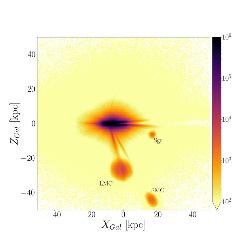
A&A 658, A91 (2022)

Table 2. Global statistics of some of the currently available astrometric and astro-photometric results based on Gaia DR2 and EDR3 data, in
comparison to this work.

            Reference                                Data used              Mag limit        # objects   σd /dG=17    σG=17
                                                                                                                       A        σG=17
                                                                                                                                 T
                                                                                                                        V         eff

            Bailer-Jones et al. (2018b)          DR2 parallaxes              G . 21            1330M       24%           –        –
            Andrae et al. (2018)               DR2 photo-astrometry          G ≤ 17             161M         –           –      324 K
                                                                                                 88M         –       0.46 mag     –
            Anders et al. (2019)             DR2 + 2MASS+AllWISE             G < 18             266M       40 %      0.25 mag   350 K
                 flag-cleaned sample             +Pan-STARRS1                                   137M       18 %      0.23 mag   230 K
            Green et al. (2019)            DR2 + 2MASS+Pan-STARRS1         zPS 1 < 20.9         799M       20 %      0.15 mag     –
            Bai et al. (2019, 2020)            DR2 photo-astrometry          G . 17             133M         –       0.16 mag   350 K
            Bailer-Jones et al. (2021)           EDR3 parallaxes             G . 21            1470M       20 %          –        –
                                              EDR3 photo-astrometry                            1310M       16 %          –        –
            This work                         EDR3 photo-astrometry         G < 18.5      402,431,354
                 StarHorse converged                +2MASS                                362,392,321      15 %      0.15 mag   183 K
                 & fidelity > 0.5                  +AllWISE                               329,646,544
                 & |C ∗ |/σC ∗ < 5               +Pan-STARRS1                             321,131,855
                 & sh_outflag==“0000”             +SkyMapper                              281,501,963

Notes. G=17 For comparability, we report here the median precision for stars at magnitude G ≈ 17.

    The second digit flags negative extinction. Significantly neg-        σAV ). The gridding effect in the metallicity panels of Fig. 3 is
ative extinctions should be treated with care: IF AV95 > 0 THEN           due to the finite resolution of the model grid.
0 ELSE 1.                                                                     Figure 4 shows the sky distribution of the input sample
    The third digit warns about very large uncertainties.                 (400 M stars with G < 18.5), as well as sky maps of the per-
Large uncertainties are not problematic per se, but the cor-              centage of converged sample and the cleaned sample. The figure
responding median values are not usually very informative,                shows that the code convergence is lowest in the densest areas
which is why we provide this flag to be able to filter                    of the sky (the innermost bulge and Galactic plane as well as
out very uncertain results quickly. The definition is as fol-             the centre of the Large Magellanic Cloud), and that cleaning the
lows: IF 0.5 ∗ (dist84 − dist16)/dist50 > 1 OR 0.5 ∗                      Gaia data enhances this effect. For example, the X shape in the
(AV84 − AV16) > 1 OR 0.5 ∗ (teff84 − teff16) > 1000 OR                    inner bulge visible in the bottom panel of Fig. 4 is mainly pro-
0.5 ∗ (logg84 − logg16) > 1 OR 0.5 ∗ (met84 − met16) > 1                  duced by the quality cut in the Gaia EDR3 colour excess factor
OR 0.5 ∗ (mass84 − mass16)/mass50 > 1 THEN 1 ELSE 0.                      (compare to Fig. 21 of Riello et al. 2021).
    The fourth digit flags very small uncertainties. Very small               In the following subsections, we present some immediate
posterior uncertainties are most likely underestimated and prob-          results that can be obtained from our catalogue, focussing on
ably indicate poor convergence. These results should also                 CMDs (Sect. 4.2), Kiel diagrams (Sect. 4.3), stellar density maps
be used with care. The definition is as follows: IF 0.5 ∗                 (Sect. 4.4), and extinction maps (Sect. 4.5).
(dist84 − dist16)/dist50 < 0.001 OR 0.5∗(av84 − av16) <
0.01 OR 0.5 ∗ (teff84 − teff16) < 20. OR 0.5 ∗                            4.2. Extinction-corrected colour-magnitude diagrams
(logg84 − logg16) < 0.01 OR 0.5 ∗ (met84 − met16) < 0.01
OR 0.5 ∗ (mass84 − mass16)/mass50 < 0.01 THEN 1 ELSE 0.                   Since the stellar models used in our Bayesian inference have not
    Unproblematic results from the point of view of StarHorse             changed much with respect to A19, the StarHorse extinction-
can thus be filtered by requiring sh_outflag==“0000”.                     corrected CMDs are also similar. The top row of Fig. 5 shows
                                                                          the CMD of the total sample and two interesting subsamples (the
                                                                          Gaia-cleaned sample and the fully flag-cleaned sample). When
                                                                          comparing these panels to Fig. 5 in A19, we note that some of
4. StarHorse Gaia EDR3 results                                            the previously noted unphysical features have disappeared (most
                                                                          notably, the ‘nose’ between the main sequence and the lower
4.1. Summary
                                                                          red-giant branch). On the other hand, new structure in the top
Table 2 summarises the results of the StarHorse run for Gaia              parts of the full CMDs emerges from the explicit inclusion of
EDR3 as well as previous results available from the recent lit-           the Magellanic Clouds in the priors. For illustration, the bot-
erature. We observe that our new StarHorse results compare                tom row of Fig. 5 shows the populations of the Milky Way disc,
favourably in terms of both sample size and parameter precision.          the Large Magellanic Cloud (LMC), and the Small Magellanic
For example, the results have notably improved in precision (typ-         Cloud (SMC).
ically shrinking the formal uncertainties by a factor of 2) with              The second row of Fig. 5 shows the CMDs for three bins in
respect to A19 (see Sect. 6 for a more detailed comparison).              apparent magnitude. The overall appearance of the magnitude-
    Figure 3 shows the distribution of the StarHorse median               binned CMDs in Fig. 5 resembles those of Fig. 4 in A19, with
posterior output values T eff , log g, [M/H], M∗ , d, and AV and          a few notable differences. For example, in addition to the sharp
their corresponding uncertainties, demonstrating the complex-             features of single-star evolution in the G < 14 panel, we now
ity of the dataset as well as the typical precision (discussed in         also appreciate the unresolved binary sequence right above the
more detail in Sect. 5.1). Even the median output parameters              low-mass main sequence. We also see the impact of the LMC
are highly correlated, either intrinsically (enforced by the stel-        and SMC populations on the CMD, already in the magnitude
lar models, e.g. T eff vs. log g), due to selection effects (e.g. d vs.   bin 16 < G < 17. The rightmost middle panel, corresponding
M∗ ), or because of degeneracies related to our method (σTeff vs.         to 18 < G < 18.5, shows already significant broadening in the

A91, page 6 of 27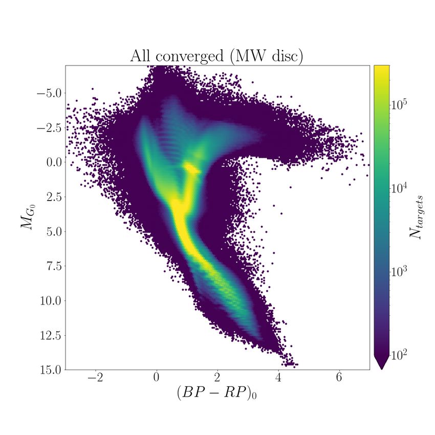
F. Anders et al.: StarHorse parameters for Gaia EDR3 stars

Fig. 3. corner plots showing the correlations and distributions of StarHorse median posterior output values T eff , log g, [M/H], M∗ , d, and AV
(lower-left panels), and their corresponding uncertainties (in logarithmic scale; top-right panels) for all stars in our catalogue. The dashed vertical
lines in the diagonal panels show the 16th, 50th, and 84th percentiles of each parameter.

CMD features. As in A19, this is a result of the growing uncer-              4.3. Kiel diagrams
tainty in the input parameters, especially the parallax. We also
recall that the absolute magnitudes and de-reddened colours dis-             Figure 6 shows Kiel diagrams (T eff vs. log g) for the full Gaia
played in Fig. 5 are not a direct output of StarHorse, but were              EDR3 StarHorse sample. The density plot (left panel) shows
computed from the observed magnitudes and the StarHorse                      that most of the sample is classified as FGK stars, as expected.
median distance, extinction, and effective temperatures4 .                   Also clearly visible (both in the left and the middle panel) are
                                                                             the stripe-like overdensities corresponding to the metallicity res-
4
    https://github.com/fjaellet/gaia_edr3_photutils                          olution of the stellar model grid already noted in Sect. 4.1.

                                                                                                                                    A91, page 7 of 27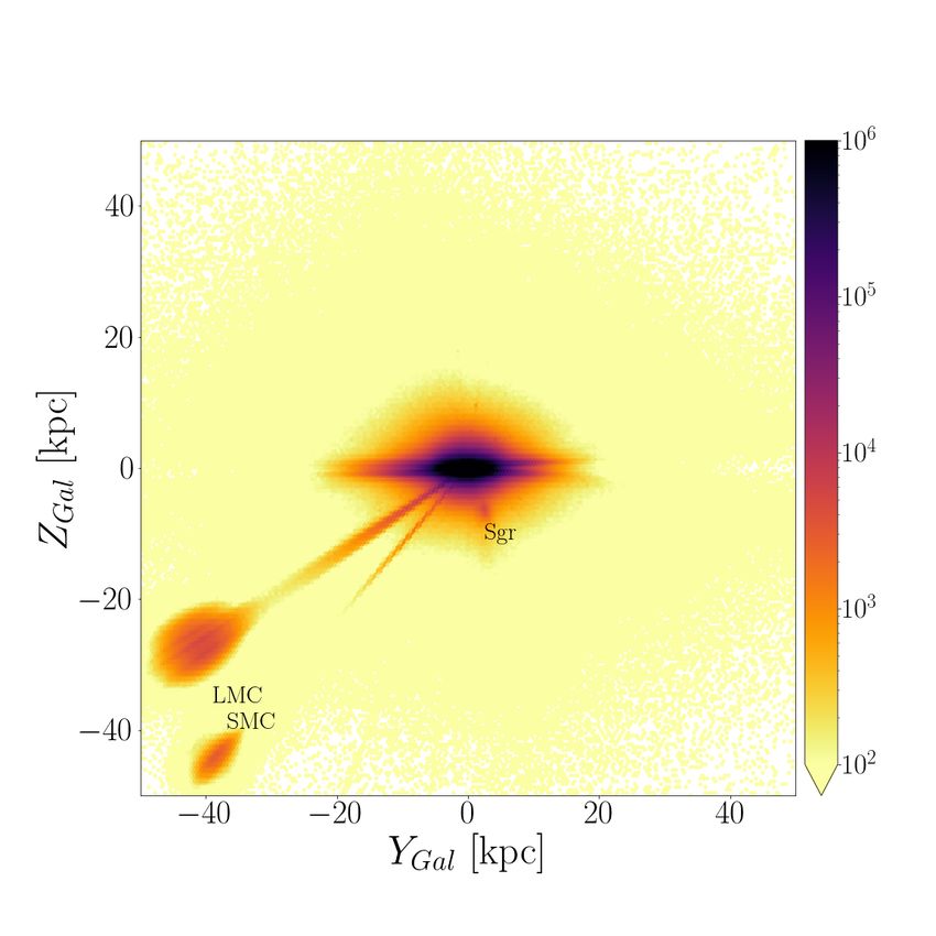
A&A 658, A91 (2022)

                                                                                           which the median StarHorse are unreliable) has diminished
                                                                                           enormously with respect to A19.
                                                                                               Finally, the right panel of Fig. 6 shows the typical distance
      180◦           90◦             0◦     360◦              270◦                 30◦     range sampled for different regions of the Kiel diagram (also
                                                                                           visible in Fig. 3), showing the expected behaviour of large typ-
                                                                                      0◦   ical distances (even >100 kpc) for the most luminous stars and
                                                                                           very small distances for the coolest and least massive dwarf stars
                                                                                   −30◦    ( 7.5 in A19).                                                                    artefacts, such as underdensities of red-clump stars both in front
    The middle panel of Fig. 6 (Kiel diagram colour-coded by                               of and behind the near side of the bar, or an underdense ring-like
metallicity) shows that the posterior metallicity information is                           structure that arose from the quality cuts necessary to clean the
consistent with the stellar model grid through most of the param-                          DR2 StarHorse data.
eter space. The only few outliers from the space spanned by                                    The EDR3 version of that figure, shown in Fig. 8, shows that
the stellar models are stars whose median output parameters lie                            the result of A19 (the detection of the Galactic bar in stellar den-
in-between the main sequence and the giant branch (due to a                                sity) is clearly maintained. The number of red-clump stars has
significantly bimodal posterior). The number of those stars (for                           become greater (13.8M vs. 10.8M), the underdensity artefacts of

A91, page 8 of 27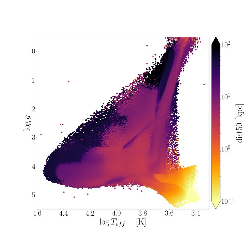
F. Anders et al.: StarHorse parameters for Gaia EDR3 stars

Fig. 5. StarHorse posterior Gaia EDR3 CMDs. Top row, from left to right: all converged objects (362M), Gaia EDR3 cleaned sample (321M),
EDR3- and flag-cleaned sample (282M). Middle row: CMDs for three broad magnitude bins, showing both the increasing mix of stellar populations
(e.g. the giant-star populations of the Magellanic Cloud starting to appear around MG ∼ −3 in the 16 < G < 17 panel) and the decreasing
astrometric quality with increasing magnitude. Bottom row: separate CMDs for the Milky Way disc (left; 339M stars), the LMC (middle; 1.09M
stars), and the SMC (right; 94k stars). The abrupt absolute magnitude cut in the last two panels is caused by the G < 18.5 mag cut.

the map are greatly reduced, and the probed Galactic area now           Castro-Ginard et al. 2021; Zari et al. 2021; Poggio et al. 2021),
extends to regions beyond the (near side of the) bar.                   and the map in Fig. 8 shows the underlying density distribu-
    The apparent bar angle is similar to the one in Fig. 8 of           tion convolved with dust extinction and other selection effects.
A19 and thus still appears to be a few degrees higher than the          The clear overdensity in the (logarithmic) red-clump star count
one assumed in the prior (27 deg; see Sect. 3.1.3). The main            map is, however, a strong feature that deserves further investi-
overdensity of the bar also appears relatively short compared           gation, since the strength of the spiral density signature in an
to recent estimates of &5 kpc. A quantitative analysis of the           intermediate-age population has implications on the modelling
bar’s structural parameters is, however, beyond the scope of this       of the Milky Way’s spiral arms.
paper, as this requires careful modelling (e.g. Wegg et al. 2015;           Recently, Nogueras-Lara et al. (2021) have used the high
Portail et al. 2017) and taking into account selection effects.         angular-resolution infrared photometric survey GALACTICNU-
    Another feature in Fig. 8 is an overdensity appearing around        CLEUS (Nogueras-Lara et al. 2019) to determine the distances,
RGal ∼ 6 kpc that might correspond to the Sagittarius spiral arm        extinctions, and stellar populations of the inner spiral arms
(see e.g. Reid et al. 2019). This feature is much less clear in the     in a small region of the sky containing the Galactic centre.
red-clump stars than in maps of young stellar populations (e.g.         While their data are of clearly superior quality, we suggest that

                                                                                                                           A91, page 9 of 27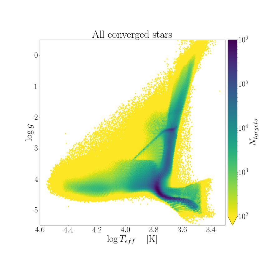
A&A 658, A91 (2022)
Fig. 6. StarHorse-derived Kiel diagrams (before applying any quality cuts). Left: density plot. Middle: colour-coded by median metallicity. Right:
colour-coded by median distance.
similar mapping studies could be carried out using Gaia and of −0.68 dex. This suggests that the little metallicity information
multi-wavelength photometry (and possibly our StarHorse cat- contained the broad-band colours we use in this work is affected
alogue) for the portions of the disc less affected by interstellar by significant systematics, at least for the very dense and com-
extinction. plex regions of the Magellanic Clouds. The declining influence
of the LMC prior biases the resulting median metallicities and
inverts the expected trend (this can possibly be remedied when
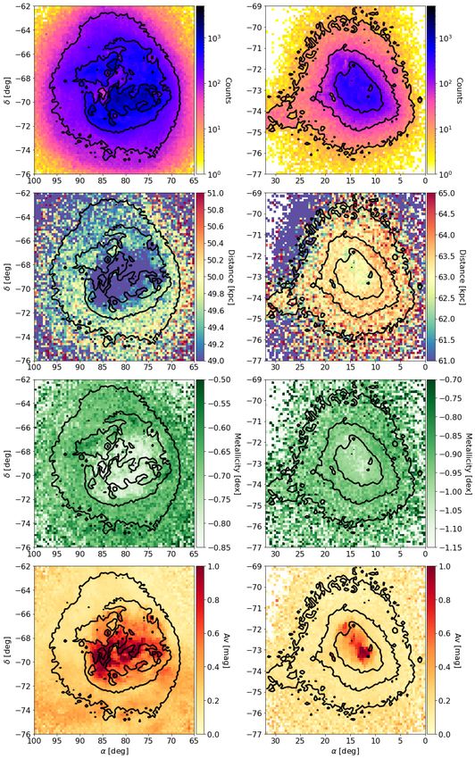
4.4.3. Magellanic Clouds using the full posterior; see Appendix B).
The Magellanic Clouds as our immediate galactic neighbours Analogously, the right column of Fig. 9 shows the corre-
represent a key laboratory to study gravitational interactions and sponding plots for the SMC sample. The sky distribution (top-
their effects on the structure and kinematics of satellite galax- right panel of Fig. 9) highlights the irregular structure of the
ies. In this section, we analyse our results for the region of the SMC and the beginning of the bridge towards the direction of
growing right ascension (and decreasing declination). The dis-
Magellanic Clouds and compare them to the Gaia Collaboration
tance map (second row right panel of Fig. 9) provides a median
(2021d) results.
distance to the SMC of 63.2 kpc (prior: dprior = 63.97 kpc), for
In Fig. 9 we show from top to bottom the sky density map, the sources inside the outermost level, in agreement with pre-
2D distance distribution, metallicity and extinction maps for the vious estimations (e.g. Cioni et al. 2000). The outer ring with
sources around the Large Magellanic Cloud (LMC, left) and closer distances may be partly an artefact due to the vanishing
Small Magellanic Cloud (SMC, right), respectively, in equato- of the prior contribution towards the outer regions. No clear dis-
rial coordinates. tance gradient is visible in the SMC.
For the LMC (left column of Fig. 9), the sky density dis- Two small blobs with slightly smaller distance are visi-
tribution highlights the main components of the galaxy. The ble in the central parts of the SMC, which are also corre-
innermost contour encloses the elongated bar, while the second lated with the metallicity. Again, a small positive metallicity
contour highlights the spiral arm. We notice a small region with gradient from the inner towards the outer parts of the galaxy
low star density between the bar and the spiral arm, in agreement is visible, opposite to the expected behaviour observed with
with the star counts shown in Gaia Collaboration (2021d, e.g.), the Red Giant Branch sources from MCPS and OGLE-III
but much less smooth, because of the relatively low convergence (Choudhury et al. 2018) or Gaia DR2 (Grady et al. 2021). As
rate of StarHorse in that region (due to crowding issues in the in the LMCANDE0890215004, the metallicity and extinction
input data; see Fig. 4). appear to be correlated, being the extinction higher towards the
The distance map (second row of Fig. 9) indicates a median central more crowded region of the galaxy (see bottom-right
heliocentric distance of 49.4 kpc (for comparison, the distance panel of Fig. 9).
used in the prior is dprior = 50.58 kpc; McConnachie 2012), for
the sources inside the outermost contour level, in agreement with 4.4.4. Candidate metal-poor stars
previous estimations (e.g. Pietrzyński et al. 2019). It also shows
the expected distance gradient from the fact that the LMC is The study of metal-poor stars provides a unique window into the
inclined about 34◦ , being the closer side the one towards larger formation and accretion history of our Galaxy, since the bulk of
declinations (Gaia Collaboration 2021d, and references therein). those stars were formed at high redshift and conserve abundance
The LMC metallicity map (third row left panel of Fig. 9) patterns unique to their site of formation (Beers & Christlieb
highlights a problematic result: In the inner parts of the LMC, we 2005).
see a positive metallicity gradient from the bar region towards Although the broad-/intermediate-band photometry used in
the outer disc, opposite to the trend observed with red-giant this work is only marginally sensitive to metallicity (in fact, only
branch (RGB) stars from Magellanic Cloud Photometric Sur- when including optical griz photometry can we expect to detect
vey (MCPS) and OGLE-III (Choudhury et al. 2016), RR Lyrae some metallicity information; see Sect. 5), low metallicities may
stars from OGLE-IV (Skowron et al. 2016), or RGB stars from manifest themselves in the broad-band colours (especially in
Gaia DR2 (Grady et al. 2021). The median metallicity in the bar the ultraviolet; e.g. Norris et al. 1999). We therefore venture to
region (inside the innermost contour level) is of −0.77 dex, while look at candidate metal-poor stars as determined by StarHorse,
at the outer disc (between the innermost and outermost levels) is by defining a candidate metal-poor sample as met84 < −1,
A91, page 10 of 27F. Anders et al.: StarHorse parameters for Gaia EDR3 stars
Fig. 7. StarHorse density maps (from top to bottom: XY, XZ, and YZ) in galactocentric coordinates. Left column: 100 kpc wide cube centred on
the Galactic centre, while right column: zooms into a 20 kpc wide cube centred on the Sun.
corresponding to a 1σ confidence-level cut. This selection yields ous structure, is also visible in the direction of the core of the Sgr
1.58 million objects (without applying any further quality cuts). dSph galaxy (located towards (l, b) ∼ (5, −14)), resulting in an
Figure 10 shows the distribution of the metal-poor candi- elongated overdensity around (RGal , ZGal ) ∼ (0 − 3, −1).
dates in galactocentric cylindrical coordinates (RGal vs. ZGal ). We Apart from these expected features, we also note a very
clearly see the imprint of the globular-cluster priors in this figure: prominent overdensity of local dwarf stars, many of them also
All noticeable point-like overdensities correspond to prominent following a disc-like density profile, and a diffuse overden-
globular clusters, as annotated in the plot. We also note the over- sity in the nearby Galactic halo. The disc-like overdensity is
densities in the direction of the Magellanic Clouds, correspond- likely mostly due to sample contamination, although even very
ing to stars with bimodal distance probability density function metal-poor stars have been found on disc-like orbits recently
(PDFs), resulting in a median distance in-between the inner halo in the Milky Way (Sestito et al. 2020) as well as in simu-
and the Magellanic Clouds (see Sect. 4.4.3). A similar, less obvi- lations (Sestito et al. 2021). The diffuse overdensity at larger
A91, page 11 of 27A&A 658, A91 (2022)
Fig. 8. XY density map, selecting all (13.8M) red-clump stars less than
3 kpc away from the Galactic midplane. The ellipse shows the orienta-
tion (27 deg with respect to the Sun-Galactic centre line) and approx-
imate extent (semi-major axes a = 4.07 kpc and b = 0.76 kpc) of the
Galactic bar assumed in the prior.
heliocentric distances is produced by more distant giant stars
of the inner halo, expected from the combination of our selec-
tion function (G < 18.5) and our halo prior. Its members can
be regarded as potential targets for future/ongoing spectroscopic
surveys. Another possible overdensity is seen in the central parts
of the Galaxy, where indeed many of the Milky Way’s oldest
stars are expected to reside (e.g. Tumlinson 2010; Koch et al.
2016; Starkenburg et al. 2017; Horta et al. 2021; Queiroz et al.
2021).
Although methods explicitly tailored to detect metal-poor
star candidates from combined broad- and narrow-band colours
can be expected to perform much better (e.g. Beers et al. 1985; Fig. 9. Median sky density, distance, metallicity, and extinction
Youakim et al. 2017; Da Costa et al. 2019; Thomas et al. 2019; maps (from top to bottom) of the Magellanic Clouds as seen by
Arentsen et al. 2020; Chiti et al. 2021; Huang et al. 2021b), our StarHorse (in equatorial coordinates and only including objects with
dist50 > 25 kpc). Left panels: centred on the LMC, right panels: on the
approach yields a large number of metal-poor star candidates for SMC. The contour lines in each of the panels are derived from the sky
possible follow-up observations with multi-object spectroscopic density plots in the top panels. For the LMC, the contours are drawn
surveys such as 4MOST (de Jong et al. 2019; Chiappini et al. at stellar densities of [100, 300, 700] per pixel (from outside inwards),
2019; Helmi et al. 2019). with 905 205 sources within the outermost contour. For the SMC, the
contour lines correspond to levels [10, 50, 200], with 195 634 sources
contained inside the outermost contour.
4.4.5. Outer halo and Local Group
Figure 11 focuses on the density distribution of distant stars in
the Galactic halo (defined by |b| > 15 deg, dist50 > 10 kpc). dSph), the more informative extragalactic priors of the new
The two top panels (showing Aitoff projections of the sky in StarHorse results can help to improve membership probabili-
ecliptic coordinates) highlight the long tidal tails of the Sgr dSph ties. For others (e.g. Sculptor dSph, Fornax dSph), the prominent
galaxy, also called the Sgr stream (e.g. Law et al. 2016). This pencil-beams between the halo and the expected location of the
feature, although not included in our priors, appears clearly both respective dwarf galaxy hint a problematic prior (e.g. imprecise
in the density map (top panel of Fig. 11) and the median distance central coordinates or too low galaxy masses in the Local Group
map (middle panel), superseding the extent of the previous mem- tables used) that results in typically bimodal distance posterior
bership maps of the Sgr stream, for example the one produced by PDFs.
Antoja et al. (2020) based on Gaia DR2 proper motions.
The lower panel of Fig. 11 shows that the G < 18.5 sam- 4.5. Extinction maps
ple encompasses also a significant amount of individual stars
in dwarf galaxies of the Local Group other than the Magel- Figure 12 shows the median StarHorse-derived line-of-sight
lanic Clouds and the Sgr dSph. For many of them (e.g. the extinction per HealPix cell in four consecutive distance bins out
Draco dSph, Bootes I, the Carina dSph, or the Ursa Minor to 2.5 kpc (from top to bottom), illustrating the gradual increase
A91, page 12 of 27F. Anders et al.: StarHorse parameters for Gaia EDR3 stars
Fig. 10. Density map for bona fide candidate metal-poor stars
(met84 < –1; 1.58M stars) in galactocentric coordinates. Some promi-
nent overdensities corresponding to Galactic globular clusters and the
direction towards the Magellanic System are annotated.
in interstellar extinction as a function of distance and sky posi-
tion. As expected, these maps are similar to the large-scale
integrated dust extinction maps of, for example, Green et al.
(2019). Since we have used the three-dimensional extinction
maps of Green et al. (2019) and Drimmel et al. (2003) (albeit
convolved with quite broad Gaussians) in our prior, this is not
too surprising.
In principle, our extinction results can be used to infer
precise distances to individual dust clouds (e.g. Wolf 1923;
Zucker et al. 2020) and to infer the three-dimensional distribu-
tion of dust (e.g. Lallement et al. 2019; Leike et al. 2020). The
top panel of Fig. 12 shows the presence of high-latitude dust
within the 500 pc sphere around the Sun, confirming that the
so-called North Polar Spur (the dust filament reaching up to
b ∼ 45 deg at l ∼ 0 deg) is a local structure and not related to
the Fermi bubbles produced by the Galactic centre (see Das et al.
Fig. 11. Distribution of distant halo stars, selected by excluding
2020 for a comprehensive discussion). the Galactic plane and a cut in median distance (|b| > 15 deg,
dist50 > 10 kpc; 2.55M stars). Top panel: sky distribution in ecliptic
coordinates, highlighting the presence of the Sagittarius stream close to
5. Precision and accuracy the ecliptic plane. Middle panel: same projection, colour-coded by the
median distance per HealPix. In both panels the contour overlay shows
5.1. Internal precision the location of the Sagittarius stream candidates from Antoja et al.
Along with the median statistics of each output parameter, (2020). The bottom panel shows a Cartesian projection (XGal vs. ZGal ),
highlighting some of the less prominent Local Group objects included
StarHorse also delivers the corresponding confidence intervals in the priors.
(defined as the 16th and 84th percentile of the marginal poste-
rior). The overall distribution of the output uncertainties (defined
as, for example, σTeff = 0.5 · (teff84 − teff16), etc.) and
the correlations between the output uncertainties are shown in nitude. In Fig. 13 we therefore show the formal uncertainties as
the top-right corner plot of Fig. 3. This plot shows the com- a function of G magnitude for a random sample of 1 million
plete sample of converged stars and demonstrates that the output stars. The orange two-dimensional histogram in the background
uncertainties are typically highly correlated (we note the loga- shows the uncertainty distribution of all objects, while the red
rithmic scaling of the plot axes). The highest correlations are line shows the smoothed median trend. We can appreciate that
seen, as expected, between effective temperature and extinction, the distance uncertainties for stars with G < 14 are typically
and between distance and surface gravity. around 2%, growing to about 8% around G ≈ 16, and reach-
The precision of the results, however, depends first and fore- ing 20% at G ≈ 18. The improvement in precision with respect
most on the quality of the Gaia EDR3 parallaxes and the avail- to our DR2 run (A19, black line in Fig. 13) is mainly due to
ability of multi-band photometry for each source. Both these the improvement in both precision and accuracy brought by the
criteria are, to first approximation, functions of the Gaia G mag- Gaia EDR3 parallaxes.
A91, page 13 of 27A&A 658, A91 (2022)
1. a slight increase of the ‘parallax sphere’ (the region for which
parallaxes are determined with a precision of .20%), 2. the dis-
appearance of the bulk of stars with very high distance uncer-
tainties that had to be flagged because they were compatible
with both dwarf- and giant-star solutions, and 3. a slightly lower
impact of the missing PS1 photometry on the T eff and AV preci-
sions below a declination of −20 deg (YGal < 0, XGal & −10 kpc)
thanks to the use of SkyMapper data (and, in fact, a higher pre-
cision in the region where both catalogues overlap).
The precision of the secondary output parameters (log g,
[M/H], and M∗ ), not shown in Table 2 and Fig. 13, behave sim-
ilarly as a function of G, although the improvement in precision
with respect to the DR2 results is slightly less pronounced (by a
factor of 1.5). At magnitude G ≈ 17, the median uncertainties for
the secondary output parameters amount to σG=17 log g = 0.23 dex,
σ[M/H] = 0.10 dex, and σ M∗ /M∗
G=17 G=17
= 9.5%.
5.2. Comparison to open clusters
Member stars of an OC are expected to have, to first order, the
same age, metallicity, distance, and interstellar extinction. They
thus constitute excellent samples fro evaluating the precision and
accuracy of our astrophysical parameters.
Figure 14 shows comparisons of the StarHorse distance,
extinction, and metallicity scales for the five most populated
and well-studied OCs (NGC 6791, NGC 7789, Collinder 261,
NGC 3532, and NGC 188) in the Gaia DR2 OC catalogue of
Cantat-Gaudin et al. (2020). These OCs are those with the most
identified members, mainly by virtue of being relatively mas-
sive and nearby (but not so nearby that they are extended in the
sky and in proper-motion space, like the Hyades). Each panel
of Fig. 14 shows a StarHorse output parameter as a function
of effective temperature in comparison to the literature values
for the particular cluster. The five clusters are diverse enough in
their physical characteristics to appreciate some first trends as
a function of effective temperature, surface gravity, metallicity,
and cluster age.
For example, for the old metal-rich cluster NGC 6791
the StarHorse-derived metallicities are clearly underestimated
(with respect to the spectroscopically derived cluster metallicity
[Fe/H]; Casamiquela et al. 2017) and show a quite large scatter
(which is, however, both expected and reflected in the quoted
uncertainties). Similarly, the code finds a slightly lower extinc-
tion and distance than derived by Cantat-Gaudin et al. (2020).
A more quantitative comparison for the bulk of the known
Galactic OC population (the 1867 OCs with astrophysical
parameters from the Cantat-Gaudin et al. 2020 catalogue) is
shown in Figs. 15 and 16. Cantat-Gaudin et al. (2020) deter-
mined the distance, extinction, and age of each cluster homoge-
neously with an artificial neural network trained on a set of high-
quality measurements (mostly relying on Bossini et al. 2019).
In Fig. 15 we plot the StarHorse median values per cluster
(for FGK-type stars, 3800 K < T eff < 6000 K) compared with
the Cantat-Gaudin et al. 2020 determinations of the distance and
Fig. 12. All-sky median StarHorse extinction map for four wide dis- extinction. The colour represents the median absolute deviation
tance bins up to 2.5 kpc, as indicated in each of the subplots. (MAD) obtained for the cluster members in SH. Figure 15 shows
that the OCs cover a broad range of physical parameters: 90% of
the clusters are nearer than 4.4 kpc and have less than 2.5 magni-
The bottom row of Fig. 13 show the median formal uncer- tudes of extinction, and the age range (10–90th percentile) cov-
tainties as a function of position in the Galaxy, again for a ers log τ from 7.2 to 9.1.
random set of 1 million stars. Many of the features in these A complementary catalogue of astrophysical parameters for
uncertainty maps can already be appreciated (although at a dif- OCs was recently presented by Dias et al. (2021). It contains
ferent absolute scale) in Fig. 13 of A19. Apart from the overall parameters of 1743 OCs (in their vast majority also contained
precision improvement (by a factor of ∼2) the major changes are: in Cantat-Gaudin et al. 2020) determined by isochrone fitting of
A91, page 14 of 27F. Anders et al.: StarHorse parameters for Gaia EDR3 stars
Fig. 13. StarHorse formal output uncertainties. Top row: uncertainties in distance (relative distance uncertainty; left), extinction (middle), and
effective temperature (right) as a function of G magnitude. In each top panel we show two-dimensional histograms of a random sample of 1 million
Gaia EDR3 stars in orange, along with the running median smoothed by an Epanechnikov kernel (width = 0.2; thick red line). For comparison
we also show the corresponding values obtained from the (unfiltered) Gaia DR2 run A19 in black, as well as the results from Bailer-Jones et al.
(2021) for distances, from Andrae et al. (2018) and Bai et al. (2020) for extinctions, and from Andrae et al. (2018) and Bai et al. (2019) for effective
temperatures. Bottom row: median formal output uncertainties as a function of Galactic position for the same random sample.
Gaia DR2 photometry. We used this catalogue as an additional In Fig. 16 we further investigate possible systematic biases
reference to test if the discrepancies between StarHorse and the depending on sky position and spectral type. We find a rather
Cantat-Gaudin et al. (2020) catalogue can partly be attributed to uniform sky distribution of relative distance differences that is
systematics in the OC catalogues as well. We only show the com- consistent with Fig. 15. The distance systematics are typically
parison with Cantat-Gaudin et al. (2020); the comparison with very small and lightly negative (.5%; see also the last row
the Dias et al. (2021) catalogue leads to the very similar general of Fig. 15). A sky pattern is hardly discernable, but may be
conclusions. related to the parallax bias present in Gaia DR2 (and thus also in
The top row of Fig. 15 shows that the concordance with the the Cantat-Gaudin et al. 2020 and Dias et al. 2021 catalogues),
OC distance scale is reasonable. The majority of both the clus- which has been largely accounted for in EDR3 (using the cor-
ters and the member stars present less than 20% deviation. The rections proposed by Lindegren et al. 2021b).
deviating clusters are mostly distant objects with very few mem- Both the parallax improvement with respect to Gaia DR2
ber stars, partly uncertain membership, and thus a large inter- and the inclusion of a dust map in the new priors allow a
nal dispersion of StarHorse parameters (red dots). We see a slightly smoother distribution of extinction differences than in
trend of negative differences with respect to the OC catalogue: A19. However, we see that extinction is generally 0.1–0.2 mag
on average, our EDR3 distances are shorter by −3.5%. An oppo- higher than the one estimated by Cantat-Gaudin et al. (2020).
site trend of similar magnitude, however, is seen in the com- Our extinction estimates are, on the other hand, slightly lower
parison with the Dias et al. (2021) catalogue: our distances are than the ones in the catalogue of Dias et al. 2021, so that the
larger than theirs by +3.8% on average. No significant trends of absolute scale is far from well defined.
distance difference with neither extinction nor age are found. Furthermore, the top-right panel of Fig. 16 shows signifi-
For extinction, on the other hand, some systematics similar to cant systematic trends of extinction with position the Kiel dia-
those seen in A19 can be appreciated: in particular, a slight sys- gram (being most severe in sparsely populated areas). For exam-
tematic overestimation for nearby, low-extinction objects. This ple, it seems that StarHorse tends to slightly underestimate
may in part be due to the fact that StarHorse treats every object extinctions for metal-rich (redder) giant stars, while it overesti-
as a single star and tries to adjust its parameters to a PARSEC mates extinctions for metal-poor giants. For dwarf stars, extinc-
isochrone. For similar-mass unresolved binaries on the main tion biases are generally low, except for (probable) binary stars
sequence this typically leads to an overestimated effective tem- close to the turn-off phase (see Appendix D.1).
perature, an underestimated log g (moving the object towards StarHorse also tends to severely overestimate the extinc-
the sub-giant or lower red-giant branch), and an overestimated tion of the stars hotter than 7000 K (Pantaleoni González et al.
extinction to compensate for the extra brightness (compared to a 2021). Due to the initial-mass-function prior, stellar models
single star). We also refer to Appendix D. with T eff & 104 K are highly suppressed in the posterior
A91, page 15 of 27You can also read