Population status and trends of Ferruginous Pygmy-owls in
←
→
Page content transcription
If your browser does not render page correctly, please read the page content below
Population status and trends of Ferruginous Pygmy-owls in
  northern Sonora Mexico: A 22 year perspective

                       Final Report

                         Prepared by:

                       Aaron D. Flesch
                      Research Scientist
       School of Natural Resources and the Environment
                    University of Arizona
           The Desert Laboratory on Tumamoc Hill
                    1675 W. Anklam Road
                      Tucson, AZ 85745
                  flesch@email.arizona.edu

                        Prepared for:

                 Tucson Audubon Society &
                   Defenders of Wildlife

                     SUMMER 2021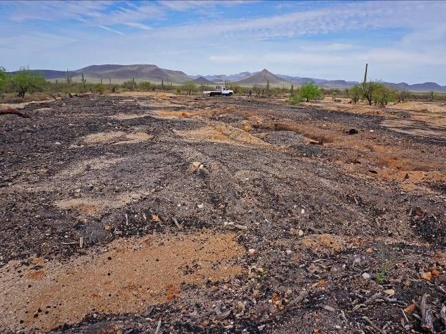
ABSTRACT

Ferruginous Pygmy-Owls (Glaucidium brasilianum) are of major conservation concern in
southern Arizona due to marked declines in distribution and abundance over the past century and
threats driven by climate and landcover change. Populations of pygmy-owls in adjacent northern
Mexico are important for recovery in the U.S. and the focus of extensive long-term monitoring
and research efforts by University of Arizona staff that began in 2000. To assess the current
status and trends of populations, I estimated abundance and territory occupancy across a vast
region of northern Sonora, Mexico immediately south of Arizona in 2021, and evaluated
spatiotemporal trends across as many as 22 years with data gathered between 2000 and 2021.
Although evidence of systematic population declines between 2000 and 2014 was strong, large
increases in abundance and occupancy in 2015-2016 eliminated statistical evidence of declining
linear trends across this time period. In 2021, however, I found that high levels of abundance and
occupancy in years 2015-2016 were not sustained, and documented marked contractions in
distribution and abundance and estimates of these parameters that were low or very low
compared to historical values for these populations. Annual estimates of territory occupancy in
2021 from a top-ranked generalized linear mixed effects model, for example, were the lowest
observed (0.435) among all 16 annual estimates across the study, and 22% lower than the long-
term average (0.560). Trend estimates for occupancy between 2001 and 2021 also provided
suggestive evidence of a systematic linear decline across the broader study area but results
depended on model assumptions. Abundance also declined markedly from levels last observed in
2015-2016, and was 6% lower than the long-term average. Such results indicate complex
population dynamics and the importance of consistently monitoring populations of concern
across time and space so that short-term changes in populations can be distinguished from long-
term declines. In 2021, I also observed a broad range of new landscape disturbances linked to
changes in land use and landcover within or immediately around many territory patches. These
changes occurred within the last ~5 years, and impacted 22% of 93 patches I surveyed in 2021,
with 29% of new disturbances at sites that had no prior impacts. Such disturbances included
vegetation clearing linked to agriculture, grazing, and woodcutting that can eliminate or degrade
pygmy-owl habitat and landscape connectivity. Historically low estimates of occupancy from
2021 together with observed impacts to habitat and anticipated increases in aridity across this
region suggest high potential for future declines of pygmy-owls in this portion of the Sonoran
Desert. Given the value and potential insights offered by long-term datasets, additional
monitoring of historical sites that are part of this program and assessment of factors that are
associated with population dynamics should be priorities for future efforts.

INTRODUCTION

The Ferruginous Pygmy-Owl (Glaucidium brasilianum; hereafter “pygmy-owl”) is an iconic
predator of the Sonoran Desert that is threatened by habitat loss, fragmentation, and degradation
linked to climate and landcover change (USFWS 2011, Flesch 2014, Flesch et al. 2015). In the
late 1800s and early 1900s, pygmy-owls were described as locally common in mesic riparian
areas in the Sonoran Desert of southern Arizona (Bendire 1888, Fisher 1893, Breninger 1898,
Gilman 1909, Bent 1938), and also occurred in woodlands along dry washes and adjacent desert
scrub (Brandt 1951, Phillips et al. 1964). By the mid-1900s, vegetation clearing for agriculture,
water diversion, and other changes in land use and landcover in wooded bottomlands drove

                                                2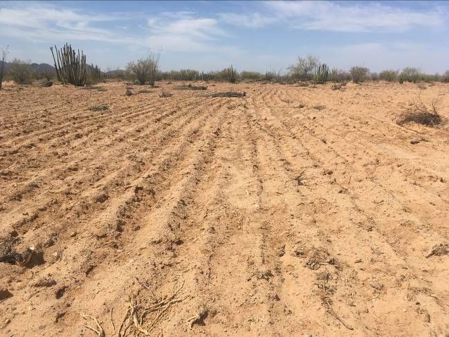
widespread habitat loss, and associated declines in distribution and abundance (Johnson et al.
2003). As a result, the Arizona population of pygmy-owls was listed as endangered by the U.S.
Fish and Wildlife Service (USFWS) in 1997, but then delisted for reasons unrelated to recovery
in 2006 (USFWS 2011). Following over a decade of litigation, populations of pygmy-owls are
now being considered for re-listing by USFWS and an ongoing species status assessment is
underway. This report includes new information on the status of pygmy-owls in the northern
Sonoran Desert that is relevant to this assessment.

Following listing and subsequent de-listing in Arizona, past monitoring suggests populations of
pygmy-owls continued to decline, but few quantitative estimates of population trends or factors
that influence them are available due to a lack of consistent and standardized monitoring. Recent
information from Arizona indicates that population units in two of the three easternmost
watershed regions in which pygmy-owls have recently occurred, in the southern Altar Valley and
near Tucson, have declined to extirpation, whereas populations in the northern Altar and Avra
valleys were stable or increasing through 2016 (Flesch et al. 2017, Flesch in revision). To my
knowledge, more recent efforts from 2020 and 2021 indicate no recent evidence of occupancy
near Tucson or in the southern Altar Valley (Arizona Game and Fish Department pers. comm.),
suggesting populations in both of these watershed regions remain extirpated. Moreover,
populations to the west in Organ Pipe Cactus National Monument seem to have also declined
recently given there were no observations of pygmy-owls between 2016 and 2020 and just two
non-breeding individuals observed in spring 2021 despite intensive survey effort by myself and
by National Park Service biologists that surveyed virtually all historical sites across the
monument (Flesch unpublished data, Flesch in prep., N.P.S. pers. comm.). Finally, recent
monitoring on Pima Country Conservation Lands in the northern Altar and adjacent Avra valleys
suggest a largely stable population on these lands, but more effort is needed to assess these
patterns given inferences are based on data from just two years (e.g., 2017, 2020; Flesch 2021).
Extensive pygmy-owls surveys by the Arizona Game and Fish Department were funded by
USFWS in years 2020 and 2021 in Arizona, and may provide quantitative inferences on the
status and trends of populations. Regardless, more field effort and especially analyses of past
survey data is required to better understand the recent status and trends of pygmy-owls in
southern Arizona.

In adjacent northern Sonora, Mexico, pygmy-owls are more common, occupy similar
environments, and systematic monitoring efforts that began in 2000 provide strong evidence that
drought and extreme temperatures are associated with marked declines in abundance (Flesch
2003, Flesch and Steidl 2006, Flesch 2014). Between 2000 and 2011, for example, abundance in
four randomly-selected watershed regions in northern Sonora declined by an estimated 19-27%,
with 75% of temporal variation in abundance explained by precipitation and temperature (Flesch
2014). Additionally, abundance was lower and varied more across time in areas with higher land-
use intensity, but abundance was higher and less variable in areas that supported more potential
nest cavities and riparian vegetation, suggesting these factors are important drivers of population
dynamics. Such patterns have alarming implications for population persistence and recovery, and
hence, data on current status and threats are critical for conservation and management.
Auspiciously, more recent monitoring in 2015 and 2016 in northern Sonora indicated substantial
increases in abundance and occupancy in these years that largely eliminated statistical evidence
of past declines (Flesch et al. 2017). Nonetheless, information on whether these levels of

                                                3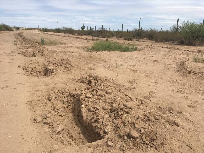
abundance persist today was unavailable, but is addressed in detail in this report. Moreover,
pygmy-owls surveys by the Arizona Game and Fish Department were funded by USFWS in year
2021 in Sonora, but the results of this work, how it was designed and implemented, and whether
it was linked to any baseline data, remain unknown, but could provide additional insights on the
status and trends of populations in the future.

With support from Tucson Audubon Society and Defenders of Wildlife in 2020, I extended
monitoring efforts for pygmy-owls in northern Sonora across one additional year so that data
now span a period of 22 years. Although planned field efforts in spring 2020 in Mexico were
cancelled due to the global pandemic, results of surveys in spring 2021 are summarized here.
Complex access and limited funding precluded surveys of all historical territories in northern
Sonora, but I surveyed all past abundance transects and a large sample of territories in April and
May 2021. Limited funding also precluded assessments of how recent changes in weather,
habitat, and landscape disturbance influenced population attributes, but I noted the presence and
type of any new changes in land use and landcover observed at and around each historical
territory patch to help evaluate current threats to habitat. Although monitoring data for pygmy-
owls had not been gathered since 2016 in northern Sonora, field work in 2021 was timely given
an ongoing status assessment of populations and threats across the northern portion of the
pygmy-owl’s range. Here I summarize information on population trends and spatiotemporal
variation in abundance and territory occupancy of pygmy-owls at the same sites between 2000
and 2021 in northern Sonora, and describe the presence and type of recent changes in land use
and landcover.

METHODS

Study Area and System—I considered populations of pygmy-owls in an approximately 20,000
km2 region of northern Sonora within approximately 125 km of Arizona (Figure 1). In Sonora, I
considered 11 watershed regions between the upper Río San Miguel watershed near Cucurpe
west to the upper Río Sonoyta watershed near Sonoyta (Figure 1). In these arid environments,
pygmy-owls are generalist predators and non-migratory residents in woodlands associated with
saguaro cacti (Carnegiea gigantea) that provide nest cavities. The study region included both
major vegetation communities occupied by pygmy-owls in the northern Sonoran Desert: the
Arizona Upland subdivision of the Sonoran Desert and semi-desert grassland (Brown 1982).
Arizona Uplands are dominated by woodlands and scrub of short leguminous trees such as
mesquite (Prosopis velutina) and saguaros. Semi-desert grasslands are dominated by open
mesquite woodlands and savannah, bunchgrasses, sub-shrubs, and saguaros are often uncommon.
Riparian areas in both communities are dominated by mesquite woodlands. Annual precipitation
in the region is bimodal and dominated by a summer monsoon in late June-Sept and winter
storms that are most intense during the warm phase of the El Niño Southern Oscillation.
Summers are hot with maximum temperatures >40°C and winters are cool with minimum
temperatures near 0°C. Throughout their range, pygmy-owls are diurnal and crepuscular
generalists that in our region prey largely on lizards during the warm season. In the Sonoran
Desert, pygmy-owls establish breeding territories in January-March, and typically lay eggs in
April and brood in May-June.

                                                 4
Figure 1. Study area in northern Sonora, Mexico showing distribution of territory patches used by Ferruginous Pygmy-
Owls. Territory patches were located in two major vegetation communities across 11 watershed regions: San Miguel,
upper Magdalena, Magdalena-Coyotillo, Busani, upper Altar, lower Altar, upper Sasabe, lower Sasabe, upper Plomo,
lower Plomo, and Sonoyta). Territory patches were 50 ha in area and are not shown to scale. Fewer watershed regions
were considered for abundance monitoring and included upper Altar, upper Sasabe, lower Sasabe, and upper Plomo.
Figure from Flesch et al. (2015).

Design and Survey Methods—Design and survey methods used during this effort have been
extensively peer reviewed and used to develop a broad range of inferences published in scholarly
journals (see Literature Cited). I estimated abundance in Sonora by repeatedly surveying the
same transects across time. In spring 2000, I surveyed 71 transects that were selected at random
in northern Sonora (see Flesch and Steidl 2006). After these initial surveys, I selected 18
transects in landscapes that were occupied by pygmy-owls at random and surveyed each transect
in spring for 15 of the next 16 years (all years except 2012) and again in 2021. All transects were
within 75 km of the U.S.-Mexico border and placed along drainage channels. To survey
transects, I placed 5-10 calling stations spaced 400 m apart along transects and broadcast
recorded, territorial vocalizations of pygmy-owls to elicit responses from owls. This method
combined with a minimum of eight minutes of survey effort at each station, the arrangement of
stations, and timing of surveys yields nearly perfect detection probability of territorial males
(Flesch and Steidl 2007). To minimize chances of double-counting individual owls that often

                                                         5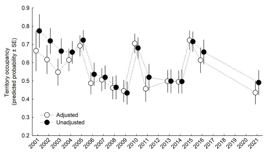
move toward broadcasts, station spacing was increased to 550-600 m after initial detection of
each male. For each owl detected, I recorded the time, distance and direction to the initial point
of detection, and the sex based on vocalization type. To estimate the number of pygmy-owls
along each transect, I used distance, timing, and direction of responses to differentiate among
multiple individuals that did not respond simultaneously. In some cases, I remained at stations
for longer than eight minutes to estimate number of respondents and returned to stations for
follow-up efforts to confirm the number of estimated individuals. As an index of abundance, I
calculated the number of territorial males along each transect in each year. All transects were
surveyed between April and early June from 1 hour before to 3 hours after sunrise. All 18
transects combined totaled 54 km in length (mean = 3.0 km, range = 2.3-3.9 km) and were
located between 740 and 1,035 m elevation.

To assess territory occupancy, I delineated individual territory patches based on patterns of space
use by owls, which I estimated with repeated surveys and nest searches (see Flesch et al. 2015).
The basic units of inference were individual territory patches that could each be occupied by
single territorial individuals or breeding pairs. To delineate territories, I surveyed transects near
random and non-random points in spring of 2000-2004, and searched for nests along occupied
transects until I located the nests of most individuals. From 2001 to 2011, 2013 to 2016, and in
2021, I surveyed areas within 300 m of most nests (or occupied areas if nests were not found
initially) known from prior years by broadcasting recorded, territorial vocalizations of pygmy-
owls in the manner described above, and through 2010 searched for nests exhaustively at nearly
all occupied sites. New territories I discovered were added to the study mainly before 2004. To
delineate territories, I plotted nest coordinates across time, identified clusters of use in space, and
placed 399-m radius circles (50 ha) around the average coordinates of each cluster, which is
similar in area to a breeding territory (Flesch et al. 2015). This approach allowed easy
identification of breeding territories because the spatial arrangement of potential nest cavities
was clumped, owls used the same general areas over time, and owl abundance peaked in early
years (Flesch 2014) when presumably most habitat was occupied.

Land-use and Landcover Change—In 2016 with help of USGS, I estimated the aerial cover of
landscape structures linked to anthropogenic land uses and landcover (see Flesch at al. 2017).
This included areas used for agriculture, housing and urban development, roadways, and other
vegetation clearings that create soil and vegetation disturbance. To estimate the location and size
of these areas, I digitized them in Google Earth during each successive year that new structures
appeared by evaluating all available imagery. I considered structures within 1 km of the center of
each territory patch to quantify land-use and landcover change both within estimated owl
territories and adjacent landscapes. To represent land use and landcover in a given year, I
considered structures that appeared between May of the prior year through April of the current
year to match the approximate phenology leading up to the breeding season. Limited support for
field work and analyses in 2021 precluded updated quantitative measures of new landscape
structures linked to anthropogenic land uses and landcover. In 2021, however, I noted the
presence and type of any new structures observed during site surveys that had occurred 5-6 years
after the last surveys, and summarized these data to evaluate changes in land use and landcover,
which could impact the quantity and quality of habitat for pygmy-owls. Because not all areas of
all territories were observed, these estimates are likely biased low.

                                                   6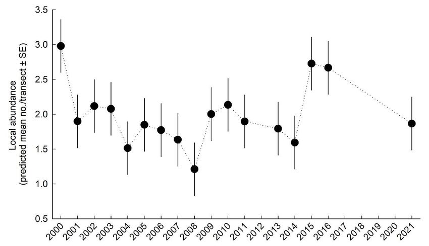
Analyses—To evaluate spatiotemporal dynamics in abundance, I used linear mixed-effects
models. I fit three models to represent different potential patterns of population dynamics and
used model selection to evaluate support among models. Each of these three models assessed a
different hypothesis regarding population dynamics. The first included a single fixed effect for
year fit across data for all four watershed regions combined to represent a single trend for the
entire population. The second included a year by watershed region interaction as fixed effects to
assess regional variation in trends. The third was an intercepts only model with no trend
parameter to represent random or other more complex variation in dynamics. To assess spatial
variation in observation error, I considered models that estimated observation variances for each
region, which was supported based on model selection. To adjust for temporal autocorrelation, I
fit first-order autoregressive correlation structures. All models included a random intercept for
transect identify because each of the 18 transects were repeatedly measured across time. As a
response variable, I log transformed estimates of the number of territorial males along each
transect. Model selection was based on Akaike information criterion adjusted for small sample
sizes (AICc) and models within 2 AICc points considered competitive for all analyses (Burnham
and Anderson 2002).

To evaluate spatiotemporal trends in territory occupancy across the broader study area, I fit
generalized linear mixed-effects models. These models fit occupancy as a binary response
variable (occupied or unobserved) with a logit link function, and different fixed effects to
represent the same three potential patterns of population dynamics assessed for abundance. This
included models with: 1) a single fixed effect for year across data for territories across all 11
watershed regions combined to represent a single trend for the entire population, 2) a model that
considered variation in trends among watershed regions with year, watershed region, and time by
region interactions fit as fixed effects, and 3) an intercepts only model with no trend parameter to
represent random or other more complex variation in dynamics. When modeling occupancy, I
included a fixed autoregressive term for occupancy state in the prior time step to account for
Markovian dependencies inherent in occupancy data. This factor adjusted for the tendency of
territories having the same occupancy status as was observed in the prior time step, which is
especially relevant in this system given site fidelity and fairly long life span of adult male
pygmy-owls. Because territories must be occupied to be discovered and included in the study, I
also censored data from the initial year each territory was discovered. Because there were gaps in
monitoring with no data gathered in 2012 and 2017-2020, 17% of observations had gaps greater
one year from the prior time step. For comparison, I also report results from models fit without
the autoregressive term for occupancy state in the prior time step. To adjust for correlations in
repeated measurements of the same territories across time and of territories embedded in the
same landscapes, I considered two potential forms of the random effects: 1) random intercept for
territory identity, and 2) random intercepts for territory and landscape identities. I based
landscapes identities (n = 39) on the proximity of territories in space, and assigned territories
located within approximately 5 km to the same landscapes, and used model selection procedures
and AICc to compare models. Annual estimates were based on least square means adjusted for all
fixed and random effects. To evaluate models and validate fit, I plotted scaled residuals against
fitted values and assessed patterns in the mean and variance of those values and presence of
outliers with large influence. Additionally, I plotted histograms of residuals and q-q plots to
visually confirm normality, and confirmed estimates of random effects variances were greater
than zero. When modeling occupancy, I assumed perfect detection probability based on evidence

                                                 7
from experimental trials (Flesch and Steidl 2007). Models for abundance were fit with nlme
library in R and those for occupancy fit with the lme4 library (Bates et al., 2015; R Core Team,
2020).
RESULTS
Effort and Observations—I surveyed abundance transects (n = 18) 306 times across 17 years that
spanned a period of 22 years from 2000 to 2021. I observed a total of 607 estimated territorial
males during these surveys and an average of 2.0 ± 0.1 males per individual transect (± SE)
survey (range = 0-8 males). With regard to territory monitoring, I surveyed an average of 90 ± 5
territory patches each year over 16 years (range = 31-108) between 2001 and 2021 for a total of
1,440 occupancy surveys across time. Effort was lowest in 2001 (31 patches) because few
patches had been identified during the initial year of study, but increased markedly each year to
2004 after which 98-108 patches were surveyed per year except in 2011 and 2016 (77) and 2021,
when I surveyed 93 patches. Raw estimates of observed territory occupancy averaged 59.1 ±
2.5% among years and ranged from a maximum of 81.6% in 2001 to a minimum of 45.3% in
2009. In 2021, observed occupancy was 50.5% or the fourth lowest value observed since 2001.
Abundance Dynamics—The intercepts only model that did not include a linear trend parameter
was the top-ranked model (Table 1). In comparison, there was limited support (ΔAICc = 1.70) for
a model that included a linear trend across time, and as in past assessments, no support for a
model with regionally varying trends (Table 1). A linear trend estimate for annual change in
abundance across time was estimated as a 0.26 ± 0.40% decline per year and was neither
statistically or biologically significant. Regardless, abundance varied widely across time and was
high initially in 2000 (least square mean = 3.0 males/transect on average), declined steadily to
2008 (1.2 males/transect), increased in 2009 and 2010 (2.0-2.1 males/transect), declined again
from 2011-2014, then increased markedly to near initial levels in 2015-2016 (2.7 males/transect;
Figure 2). In 2021, abundance declined markedly from levels last observed in 2015-2016 and
was 6% lower than the long-term average estimate of 2.0 males/transect (Figure 2).
Territory Occupancy Dynamics—Across a much broader area of 11 watershed regions,
occupancy dynamics were fairly similar to those for abundance, but results depended somewhat
on model assumptions. The intercepts only model that did not include a linear trend parameter
was the top-ranked model but only when an autoregressive parameter for occupancy state in the
prior time step was considered (Table 1). In comparison, there was also some support (ΔAICc =
0.65) for a model that included a linear trend across time, but in contrast to past assessments, no
support for a model with regionally varying trends (Table 1). After adjusting for occupancy state
in the prior time step, a trend estimate for change in the odds of occupancy was estimated as a
1.4 ± 1.2% decline per year, but was not statistically significant (P = 0.24). Occupancy state in
the prior time step had major impacts on observed occupancy in the current year and reduced
AICc by ~60 points; odds of occupancy were 3.1 ± 1.2 times higher when a territory was
occupied in the prior time step. In general, including occupancy in the prior time step as a
covariate adjusted annual estimates of occupancy probability down but mainly just during the
first three years of study, which is when most new territories were added to the study. When
occupancy in the prior time step was not included, evidence of a decline in occupancy increased
8Table 1: Rankings and descriptions of models of spatiotemporal variation in abundance and territory
occupancy of Ferruginous Pygmy-Owls in northern Sonora, Mexico between 2000 and 2021. Abundance
models consider data from 18 transects in four watershed regions gathered between 2000 and 2021, and are
based on linear mixed effects models with abundance (log no. of territorial males) fit as the response variable
and transect identity fit as a random intercept. Occupancy models consider data from 112 territories across 30
landscapes in 11 watershed regions gathered between 2001 and 2021 and are based on generalized linear
mixed effects models with occupancy (occupied or unoccupied) fit as the response variable and territory and
landscape identity fit as random intercepts. Each set of models consider different fixed effects including year,
watershed region, and their interaction fit as fixed effects, and a null model with intercepts only. One set of
occupancy models includes an autoregressive parameter for occupancy state in the prior time step to adjust
for Markovian dependencies inherent in occupancy data.
Parameter
Model {terms} K AICc ΔAICc wi
Abundance
Null model {intercepts only} 7 244.90 0.00 0.70
One population with equal trend {Year} 8 246.61 1.70 0.30
Regional variation in trends {Year + Region + Region × Year} 14 256.46 11.56 0.00
Occupancy with autoregressive parameter
Null model {intercepts only} 4 1700.91 0.00 0.58
One population with equal trend {Year} 5 1701.56 0.65 0.42
Regional variation in trends {Year + Region + Region × Year} 25 1713.29 12.38 0.00
Occupancy without autoregressive parameter
One population with equal trend {Year} 4 1765.24 0.00 0.52
Regional variation in trends {Year + Region + Region × Year} 24 1766.18 0.94 0.32
Null model {intercepts only} 3 1767.61 2.37 0.16
greatly (Table 1), and a trend estimate for change in the odds of occupancy was estimated as a
2.4 ± 1.2% decline per year, which was statistically significant (P = 0.035). Annual occupancy
probabilities across all territories varied widely across time and were high initially in 2001,
generally declined to 2009, increased in 2010, were much lower from 2011-2014, then increased
markedly to near initial levels in 2015 and 2016 (Figure 3). In 2021,occupancy probability
declined markedly from levels last observed in 2015-2016 (Figure 3). After adjusting for the
effects of occupancy state in the prior time step, annual estimates of occupancy probability in
2021 were the lowest observed (e.g., 0.435 ± 0.063) across all 16 years of study, and 22% lower
than the long-term average estimate of 0.560. When unadjusted for occupancy state in the prior
time step, annual estimates of occupancy probability in 2021 were the third lowest observed
(e.g., 0.490 ± 0.066) across all 16 years of study, and 18% lower than the long-term average
estimate of 0.597. On the raw observed scale, annual occupancy probability in 2021 (0.505) was
15% lower than the long-term average estimate of 0.591. Interestingly, estimates of occupancy
were only moderately correlated with estimates of abundance (r = 0.50, P = 0.05), likely because
the study area in which I measured occupancy was much larger than that for abundance.
9Figure 2: Trends in abundance of Ferruginous Pygmy-Owls along 18 transects (54 km) in northern Sonora, Mexico, 2000-
2021. Estimates are mean number of males per transect and are least square means form a linear mixed effects model of
log abundance that were back-transformed.
Figure 3: Trends in territory occupancy of Ferruginous Pygmy-Owls in northern Sonora, Mexico, 2001-2021. Estimates
are least-square means from a generalized linear mixed effects model that fit year as a nominal factor. Between 31 and
108 territory patches were surveyed each year. Adjusted estimates consider the effects of a first-order autoregressive
term for occupancy state in the prior time step.
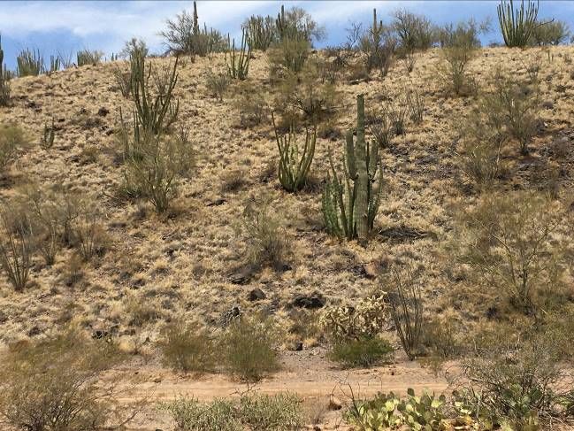
10Figure 4: Examples of landcover change and landscape disturbance at and around territories of Ferruginous Pygmy-
Owls I monitoring in northern Sonora, Mexico, 2001-2021. Clockwise from top left show clearing and plowing of desert-
scrub, presumably to encourage grass growth for grazing, remains of a charcoal operation that involves clearing and
burn pits, buffelgrass invasion on hillside among succulents, and clearing and “pitting” for pipeline installation along
Mexico Route 2.
Land-use and Landcover Change—In 2021, I observed new changes in land use or landcover
within or immediately around 20 of the 93 (21.5%) territory patches I surveyed. These changes
occurred sometime since the last survey of territory patches in 2015 or 2016 that averaged 5.2 ±
0.1 years. Territories that experienced new changes in land use and landcover since 2015 or 2016
were not always those that had the greatest levels of prior disturbance (P ≥ 0.39, t-tests),
indicating a range of less disturbed sites experienced new disturbances. Nine of the 20 territories
that experienced new changes in land use or landcover, for example, had no prior disturbances
when last surveyed across a period of more than a decade of surveys. Moreover, 31 of 93
territories we surveyed in 2021 had no prior disturbances, and 9 of these experienced new
changes in land use or landcover. Most new changes in land use or landcover were characterized
by general vegetation clearing (n = 11 territories or 58%), with lesser frequencies of new more
intensive grazing activities and grazing infrastructure (16%), mining (11%), woodcutting (11%),
or water diversion (5%). More specifically, new vegetation clearings I observed were linked to a
variety of land uses including agriculture (n = 2 territories), clearing for unknown reasons (n =
112), buffelgrass planting (n = 1), or pipeline (n = 1), check-dam type water catchment (n = 1), or
intensive woodcutting (n = 1). Examples of some of the types of landcover change I observed in
2021 at and around territories are shown in Figure 4.
DISCUSSION
Population monitoring is an essential component of wildlife conservation and management,
especially for species of conservation concern such the Ferruginous Pygmy-Owl. This report
summarizes efforts to monitor populations of Ferruginous Pygmy-Owls in northern Sonora,
Mexico that began in 2000 and continued in 2021 following a 4-year gap in field work from
2017 to 2020. Although past monitoring through 2014 indicated marked systematic declining
trends in abundance and occupancy that conform generally to findings after years 2005 and 2011
(Flesch and Steidl 2006, Flesch 2014, 2015), results after the 2015-2016 breeding seasons found
little evidence of a declining linear trend across a vast area of northern Sonora, Mexico between
2000 and 2016 (Flesch et al. 2017). This more auspicious pattern was driven by large increases
in abundance and territory occupancy in 2015 and 2016, which in a statistical sense largely
eliminated evidence of a declining linear trend model over the entire time period. Results
summarized here that include data from the 2021 breeding season, however, show marked
declines of similar magnitude in both abundance and occupancy probability in year 2021
compared to estimates from 2015 and 2016, and were generally low in a historical sense for
these populations, especially for occupancy. For example, estimates of territory occupancy based
on a model with the highest observed support, were the lowest observed across all 16 years of
study (e.g., 0.435) and 22% lower than the long-term average. Moreover, trend estimates for
occupancy provided some suggestive evidence of declines, but this model did not account for
autocorrelation in successive occupancy estimates across time, which is an important property of
these time-series data. Abundance also declined markedly from levels last observed in 2015-
2016 and was 6% lower than the long-term average. Such results indicate complex population
dynamics and the importance of consistently monitoring populations of conservation concern
across time and space so that short-term changes in populations can be distinguished from
systematic long-term declines. Additional survey work commissioned by USFWS in Sonora
2021, which may or may not be available in the future, may shed additional light on the status of
pygmy-owl populations in northern Sonora, but lacking any baseline for comparison is unlikely
to provide any inferences on population trends.
Despite limited evidence of statistically significant declining linear trends in abundance or
occupancy across the study region and time period considered here, such declines are likely to
develop in the future. This is because populations are expected to respond to increases in habitat
loss and degradation, including those documented here, and because aridity is predicted to
increase across much of the region (Cook et al. 2015, Pascale et al. 2017, Williams et al. 2020).
These stressors both individually and in combination can have negative impacts on populations
(Flesch 2014, Flesch et al. 2015, 2017). Additional monitoring and research are needed to assess
whether these anticipated declines materialize, and to apply the more than two decades of
monitoring from northern Mexico into an analytical framework to assess the drivers of
population dynamics.
12Although beyond the scope of this report, understanding factors that explain spatiotemporal
variation in abundance and territory occupancy is fundamental for guiding management and
conservation, and for evaluating why population parameters were generally low in 2021. Recent
studies of population dynamics (e.g., Flesch 2014, Flesch et al. 2017) and reproductive output
(e.g., Flesch et al. 2015) of pygmy-owls provide strong evidence that precipitation and
temperature are major drivers of carrying capacity and population processes in this system. This
is because in arid environments, precipitation can drive rapid increases in plant biomass, seed
production, and insect abundance, and create resource pulses that directly bolster food
availability for small vertebrates and subsequently for predators such as pygmy-owls (Lima et al.
2002, Holmgren et al. 2006). Predator populations such as pygmy-owls often respond indirectly
to these resources pulses at somewhat longer lag times of two or more years (Jaksic et al. 1992,
Dennis and Otten 2000, Letnic et al. 2005, Flesch 2014). Moreover, hot temperatures can have
indirect effects on populations of pygmy-owls by affecting activity or abundance of food
resources such as lizards, or direct physiological effects such as heat stress. Marked increases in
pygmy-owl populations I observed in 2015 and 2016, for example, were likely due to relatively
high levels of precipitation during the 2014 monsoon seasons and in fall 2014 when several
tropical storms of Pacific origin made landfall in the region. Much lower estimates in 2021 are
likely due, in part, to average precipitation in late 2019 through mid-2020 and to extreme
drought in late 2020 and early 2021. These recent droughts may continue to negatively impact
pygmy-owl populations into the 2022 breeding season and beyond, especially given lagged
effects observed during prior work (Flesch 2014). More broadly and of long-term concern,
observed negative effects of high temperature and low precipitation have alarming implications
for pygmy-owl in the Sonoran Desert given future forecasts associated with climate change. This
is because drought is predicted to dominate future climates of southwestern North America
(Seager et al. 2007, Cook et al. 2015, Pascale et al. 2017, Williams et al. 2020), which could
drive prolonged ecological crunches that augment extinction risk for pygmy-owls, especially in
landscapes where habitat loss and degradation are high (Maron et al. 2015, Flesch 2014, Flesch
et al 2017).
In 2021, I observed a broad range of new landscape disturbances linked to changes in land use
and landcover within or immediately around territory patches, which had occurred within the last
approximately five years. These new disturbances affected a relatively large number of territory
patches I considered during 2021 (e.g., 22% of 93 patches) despite the relatively short time
period, and fact that much of the study area includes vast open space with very low human
population densities. Such impacts were not limited only to areas that had histories of prior
disturbance, with only 29% of new impacts at sites that had evidence of past disturbances. Many
of these impacts included vegetation clearing linked to agriculture, grazing, and woodcutting.
Discussions with local landowners indicated that the ongoing drought has affected traditional
livelihoods and incomes in the region, and driven a need for new sources of income. Hence,
evidence of new more extensive woodcutting and charcoal production, new grazing
infrastructure, and efforts to clear native vegetation, which is thought to increase grass
production, seem to be a result of climate change. Such impacts are likely to have compounding
negative effects on habitat and pygmy-owl populations given a range of past observations. For
example, past work in this system has found that occupancy declines markedly as territories and
the landscapes surrounding them became increasing dominated by anthropogenic land uses and
landscape disturbance (Flesch et al. 2017, Flesch in revision). Such patterns are not surprising
13given well-known impacts of land-use and landcover change on the quantity, quality, and
connectivity of habitats, which simultaneously influence both abundance and movement of
potential colonists, reduce colonization rates, and promote edge effects and other stressors that
augment extinction risk (Hanski and Gaggiotti 2004, Fischer and Lindenmayer 2007,
Lindenmayer and Fischer 2013). Moreover, such impacts can directly interact with other
stressors such as climate change. For example, occupancy of pygmy-owl territories imbedded in
increasingly disturbed landscapes declined at greater rates with warming winter air temperatures,
which had little effect in intact landscapes suggesting they buffer the impacts of climate warming
on populations (Flesch et al. 2017, Flesch in revision). Due likely to a combination of these
stressors, populations of pygmy-owls in regions that have experienced the greatest increases in
anthropogenic disturbance in Arizona have declined to extinction (Flesch et al. 2017). Such
patterns mirror past population declines that occurred across a much larger region of southern
Arizona over the past century (Johnson et al. 2003, USFWS 2011), during which the northern
edge of the range of pygmy-owls contracted south by approximately 150 km. Monitoring
changes in land use and landcover within pygmy-owl habitat in this region is important for
understanding likely future changes to pygmy-owl populations and recovery potential. Future
work should quantify these changes using satellite imagery and integrate these data into models
of population dynamics.
Population trends of pygmy-owls in northern Sonora, Mexico have important management and
recovery implications in Arizona where pygmy-owls are of major conservation concern. Natural
or facilitated dispersal of juveniles and adult pygmy-owls from Mexico was identified among the
preferred alternatives for recovery compared to captive propagation (USFWS 2003, pg. 123).
This later technique was considered feasible only after all other techniques to maintain or
improve populations had failed (USFWS 2003, pg. 123), but inexplicably continues to be a
major focus of state and federal agencies despite little or no evidence of success and high cost. If
populations of pygmy-owls in northern Sonora decline, recovery strategies that rely on
individuals from Mexico may be jeopardized. Efforts to conserve, enhance, and create habitat for
pygmy-owls will likely have much higher potential for success. This is especially the case when
efforts are focused in areas with nearby populations within dispersal range, or when combined
with facilitated dispersal of wild birds. Such efforts and others can be guided by broad sets of
detailed inferences on habitat quality, population dynamics, habitat selection, dispersal, and
movement gathered by University of Arizona researches for nearly two decades (see Literature
Cited). To this end, promoting abundances of potential nest cavities, structural complexity and
cover of riparian woodlands, reducing deleterious changes in land use and landcover, and
promoting landscape connectivity through high levels of woody vegetation cover and large
unfragmented woodlands will enhance reproductive performance, movement, and population
growth by pygmy-owls (Flesch 2014, 2017, Flesch et al. 2010, 2015, Flesch and Steidl 2010).
ACKNOWLEDGEMENTS
I thank Tucson Audubon Society and Defenders of Wildlife for supporting field work in Mexico
and trends analyses in 2021. In past years, the U.S. National Park Service, Desert Southwest
Cooperative Ecosystem Studies Unit, U.S. Geological Survey, Tucson Audubon Society,
Defenders of Wildlife, Arizona Department of Transportation, U.S. Fish and Wildlife Service
14(2000-2002 only), T&E Inc., Center for Biological Diversity, Shared Earth Foundation, Arizona
Zoological Society, and Sierra Club provided support for population monitoring in Sonora. I
thank the many field assistants that helped with surveys in Sonora over many years and biologist
Gregorio Belmonte Herrera for assisting in 2021. Bryan Bird, Rob Peters, and Carol Beidleman
of Defenders of Wildlife provided helpful reviews and comments on a draft of this report. I thank
Christina McVie of Tucson, Arizona for helping me find funding to support this effort in 2020
after we learned U.S. Fish and Wildlife Service was initiating a species status assessment for the
pygmy-owl and had commissioned monitoring work in Sonora that included no support for this
long-term effort. Without that support, 2021 efforts would not have been completed.
LITERATURE CITED
Bendire, C.E. 1888. Notes on the habits, nests, and eggs of the genus Glaucidium Boie. Auk 5,
366-372.
Bent, A.C. 1938. Life histories of North American birds of prey, part 2. U.S. National Museum
Bulletin 170.
Brandt, H. 1951. Arizona and its bird life. The Bird Research Foundation, Cleveland, OH.
Breninger, G.F. 1898. The ferruginous pygmy-owl. Osprey 2, 128.
Brown, D.E. (editor). 1982. Biotic communities of the American Southwest: United States and
Mexico. Desert Plants 4, 1–342.
Burnham, K.P., and D.R. Anderson. 2002. Model selection and multimodel inference: a practical
information-theoretic approach. Springer-Verlag, New York.
Cook, B. I., Ault, T. R., & Smerdon, J. E. 2015. Unprecedented 21st century drought risk in the
American Southwest and Central Plains, Science Advances, 1, 1-7, e1400082.
Cook, B.I., Ault, T.R., and Smerdon J.E. 2015. Unprecedented 21st century drought risk in the
American Southwest and Central Plains, Science Advances, 1, 1-7, e1400082
Dennis, B, and M.R.M. Otten. 2000. Joint effects of density dependence and rainfall on
abundance of San Joaquin kit fox. Journal of Wildlife Management 64, 388-400.
Fischer, J. and Lindenmayer, D.B. 2007 Landscape modification and habitat fragmentation: a
synthesis. Global Ecology and Biogeography, 16, 265-280.
Fisher, A.K. 1893. The hawks and owls of the U.S. in relation to agriculture. U.S. Department of
Agriculture Division of Ornithology and Mammalogy Bulletin 3, 1-210.
Flesch, A.D., 2003. Distribution, abundance, and habitat of cactus ferruginous pygmy-owls in
Sonora, Mexico. M.S. Thesis, University of Arizona, Tucson, AZ.
15Flesch, A. D. 2014. Spatiotemporal trends and drivers of population dynamics in a declining
desert predator. Biological Conservation 175:110-118.
Flesch, A. D. 2015. Extinction risk and conservation guidelines for endangered pygmy-owls in
the Sonoran Desert. Final unpublished report to Shared Earth Foundation.
Flesch, A.D. 2021. Cactus Ferruginous Pygmy-Owl monitoring and habitat on Pima County
Conservation Lands. Report to Pima County Office of Sustainability and Conservation,
University of Arizona, School of Natural Resources and the Environment. Contract No. CT-
SUS-20-195.
Flesch, A. D., and R. J. Steidl. 2006. Population trends and implications for monitoring cactus
ferruginous pygmy-owls in northern Mexico. Journal of Wildlife Management 70:867-871.
Flesch, A.D., and R. J. Steidl. 2007. Detectability and response rates of ferruginous pygmy-owls.
Journal of Wildlife Management 71: 981-990.
Flesch, A.D., C.W. Epps, J.W. Cain, M. Clark, P.R. Krausman, and J.R. Morgart. 2010. Potential
effects of the United States-Mexico border fence on wildlife. Conservation Biology 24, 171-
181.
Flesch, A.D., and R. J. Steidl. 2010. Importance of environmental and spatial gradients on
patterns and consequences of resource selection. Ecological Applications 20:1021-1039.
Flesch, A. D., R.L. Hutto, W. J. D. van Leeuwen, K. Hartfield, and S. Jacobs. 2015. Spatial,
temporal, and density-dependent components of habitat quality for a desert owl. PLOS ONE
10(3): e0119986
Flesch, A.D, P. Nagler, and C. Jarchow. 2017. Population trends, extinction risk, and
conservation guidelines for ferruginous pygmy-owls in the Sonoran Desert. Final report for
Science Support Partnership Project for U.S. Geological Survey and U.S. Fish and Wildlife
Service. Cooperative Agreement No. G15AC00133
Gilman, M.F. 1909. Some owls along the Gila River of Arizona. Condor 11, 145-150.
Hanski I., and Gaggiotti O.E. 2004. Ecology, genetics and evolution of metapopulations.
Elsevier Academic Press.
Holmgren, M., Stapp, P., Dickman, C.R., Gracia, C., Graham, S., Gutiérrez, J.R., Hice, C.,
Jaksic, F., Kelt, D.A., Letnic, M. and Lima, M. 2006. Extreme climatic events shape arid and
semiarid ecosystems. Frontiers in Ecology and the Environment 4, 87-95.
16Jaksic, F.M., J.E. Jimenez, S.A. Castro, and P. Feinsinger. 1992. Numerical and functional-
response of predators to a long-term decline in mammalian prey at a semiarid Neotropical
site. Oecologia 89, 90-101.
Johnson, R.R., Cartron, J.L.E., Haight, L.T., Duncan, R.B. and Kingsley, K.J., 2003. Cactus
ferruginous pygmy-owl in Arizona, 1872–1971. The Southwestern Naturalist, 48, 389-401.
Letnic, M., B. Tamayo, and C.R. Dickman. 2005. The responses of mammals to La Niña-
associated rainfall, predation, and wildfire in central Australia. Journal of Mammalogy 86,
689-703.
Lima, M., N.C. Stenseth, and F.M. Jaksic. 2002. Food web structure and climate effects on the
dynamics of small mammals and owls in semi-arid Chile. Ecology Letters 5, 273-284.
Lindenmayer, D.B. and Fischer, J., 2013. Habitat fragmentation and landscape change: an
ecological and conservation synthesis. Island Press.
Maron, M., McAlpine, C. A., Watson, J. E., Maxwell, S., & Barnard, P. 2015. Climate‐induced
resource bottlenecks exacerbate species vulnerability: a review. Diversity and Distributions
21:731-743.
Pascale, S., Boos, W.R., Bordoni, S., Delworth, T.L., Kapnick, S.B., Murakami, H., Vecchi,
G.A. and Zhang, W., 2017. Weakening of the North American monsoon with global
warming. Nature Climate Change. doi:10.1038/nclimate3412.
Phillips, A.R., J.T. Marshall, Jr., and G. Monson. 1964. The birds of Arizona. University of
Arizona Press, Tucson, Arizona.
Seager, R., Ting, M., Held, I., Kushnir, Y., Lu, J., Vecchi, G., Huang, H.P., Harnik, N., Leetmaa,
A., Lau, N.C. and Li, C. 2007. Model projections of an imminent transition to a more arid
climate in southwestern North America. Science 316, 1181-1184.
Stenseth, N.C., A. Mysterud, G. Ottersen, J.W. Hurrell, K.S. Chan, and M. Lima. 2002.
Ecological effects of climate fluctuations. Science 297, 1292–1296.
U.S. Fish and Wildlife Service. 2003. Cactus ferruginous pygmy-owl (Glaucidium brasilianum
cactorum) draft recovery plan. Albuquerque, New Mexico, USA.
U.S. Fish and Wildlife Service. 2011. 12-Month finding on a petition to list the Cactus
Ferruginous Pygmy-Owl as threatened or endangered with critical habitat; proposed rule,
October 5, 2011. Federal Register 76:61856–61894.
Williams, A. P., Cook, E. R., Smerdon, J. E., Cook, B. I., Abatzoglou, J. T., Bolles, K., ... &
Livneh, B. 2020. Large contribution from anthropogenic warming to an emerging North
American megadrought. Science, 368(6488), 314-318.
17You can also read