Post-flight analysis of detailed size distributions of warm cloud droplets, as determined in situ by cloud and aerosol spectrometers
←
→
Page content transcription
If your browser does not render page correctly, please read the page content below
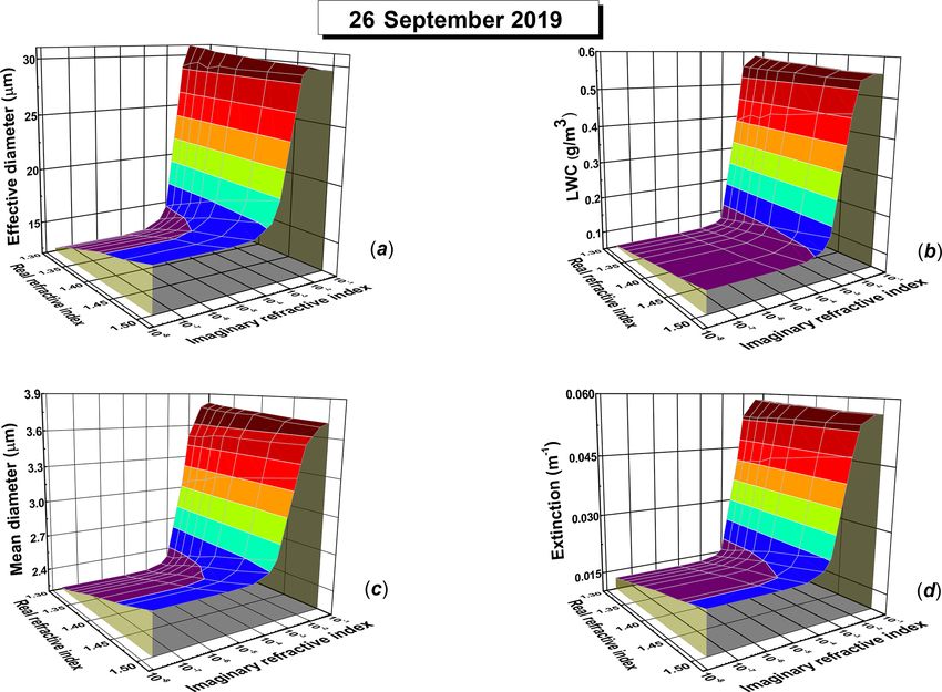
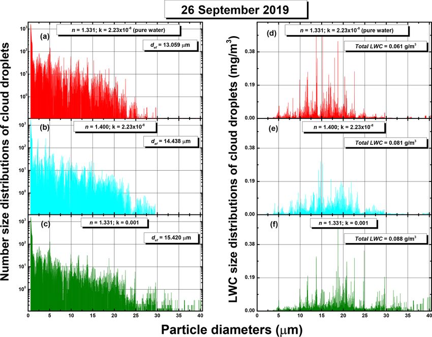
Atmos. Meas. Tech., 14, 6777–6794, 2021
https://doi.org/10.5194/amt-14-6777-2021
© Author(s) 2021. This work is distributed under
the Creative Commons Attribution 4.0 License.

Post-flight analysis of detailed size distributions of warm cloud
droplets, as determined in situ by cloud and aerosol spectrometers
Sorin Nicolae Vâjâiac1 , Andreea Calcan1 , Robert Oscar David2 , Denisa-Elena Moacă1,3 , Gabriela Iorga3,4 ,
Trude Storelvmo2 , Viorel Vulturescu5 , and Valeriu Filip1,6,7
1 Flow Physics Department, National Institute for Aerospace Research “Elie Carafoli”, Bucharest, Romania
2 Department  of Geosciences, University of Oslo, Oslo, Norway
3 Faculty of Physics, University of Bucharest, P.O. Box MG-11, Magurele, 077125, Bucharest, Romania
4 Faculty of Chemistry, Department of Physical Chemistry (Physics Group), University of Bucharest,

Bd. Regina Elisabeta 4–12, 030018, Bucharest, Romania
5 Theory of Mechanisms and Robots Department, Politehnica University of Bucharest,

Faculty of Industrial Engineering and Robotics, Bucharest, Romania
6 Graduate School of Physics, University of Bucharest, Bucharest, Romania
7 Research Center for Surface Science and Nanotechnology, University POLITEHNICA of Bucharest, Bucharest, Romania

Correspondence: Sorin Nicolae Vâjâiac (vajaiac.sorin@incas.ro) and Valeriu Filip (vfilip@gmail.com)

Received: 24 June 2021 – Discussion started: 30 July 2021
Revised: 7 September 2021 – Accepted: 20 September 2021 – Published: 21 October 2021

Abstract. Warm clouds, consisting of liquid cloud droplets,      diameter values. The optimal resolution required for con-
play an important role in modulating the amount of incoming      structing the diagram of this relationship is therefore ana-
solar radiation to Earth’s surface and thus the climate. The     lyzed. Cloud particle statistics are further assessed using a
size and number concentration of these cloud droplets control    fine grid of particle diameters in order to capture the finest
the reflectance of the cloud, the formation of precipitation     details of the cloud particle size distributions. The possibil-
and ultimately the lifetime of the cloud. Therefore, in situ     ity and the usefulness of using coarser size grids, with ei-
observations of the number and diameter of cloud droplets        ther uneven or equal intervals, is also discussed. For coarse
are frequently performed with cloud and aerosol spectrom-        equidistant size grids, the general expressions of cloud mi-
eters, which determine the optical diameters of cloud par-       crophysical parameters are calculated and the ensuing rela-
ticles (in the range of up to a few tens of micrometers) by      tive errors are discussed in detail. The proposed methodol-
measuring their forward-scattering cross sections in visible     ogy is further applied to a subset of measured data, and it
light and comparing these values with Mie theoretical com-       is shown that the overall uncertainties in computing various
putations. The use of such instruments must rely on a fast       cloud parameters are mainly driven by the measurement er-
working scheme consisting of a limited pre-defined uneven        rors of the forward-scattering cross section for each particle.
grid of cross section values that corresponds to a theoreti-     Finally, the influence of the relatively large imprecision in
cally derived uneven set of size intervals (bins). However, as   the real and imaginary parts of the refractive index of cloud
more detailed structural analyses of warm clouds are needed      droplets on the size distributions and on the ensuing cloud
to improve future climate projects, we present a new nu-         parameters is analyzed. It is concluded that, in the presence
merical post-flight methodology using recorded particle-by-      of high atmospheric loads of hydrophilic and light-absorbing
particle sample files. The Mie formalism produces a com-         aerosols, such imprecisions may drastically affect the relia-
plicated relationship between a particle’s diameter and its      bility of the cloud data obtained with cloud and aerosol spec-
forward-scattering cross section. This relationship cannot be    trometers. Some complementary measurements for improv-
expressed in an analytically closed form, and it should be       ing the quality of the cloud droplet size distributions obtained
numerically computed point by point, over a certain grid of      in post-flight analyses are suggested.

Published by Copernicus Publications on behalf of the European Geosciences Union.
6778                                                    S. N. Vâjâiac et al.: Post-flight analysis of detailed size distributions

1   Introduction                                                   value of the cross section corresponds in most cases to sev-
                                                                   eral diameters. Partly to alleviate this drawback, and partly to
Understanding the microphysics of clouds is a key compo-           accelerate the (in-flight) comparison step, the size distribu-
nent both in assessing future climate change and in opera-         tion is commonly constructed over a limited partition of un-
tional weather forecast, with vast implications for modern         even widths called bins. The limits of each size bin should be
domestic activities ranging from agriculture to energy har-        established unambiguously, in the sense that to each bound-
vesting and aviation. The cloud droplet size distribution has      ary corresponds a FWSCS value, or threshold, which cannot
long been recognized as particularly important for the Earth’s     be assigned to any other diameter of a pure water sphere. The
energy balance through the so-called cloud albedo effect           user has some freedom in setting the limits of the size bins,
(Twomey, 1977). The in-cloud microphysical processes in-           but the choice should be made in such a way that the cor-
volved in this effect are strongly influenced by the spatiotem-    responding thresholds of FWSCS are all unambiguous. The
poral variation in the detailed shape of the cloud droplet size    result is a partition of the FWSCS range in an equal num-
distribution (see, for example, Feingold et al., 1997; Liu and     ber of uneven intervals, or cross section bins, associated with
Daum, 2002; Iorga and Stefan, 2007; Liu et al., 2008; Chen         the chosen structure of the size bins. During the in-flight data
et al., 2016). It is currently recognized that in situ measure-    acquisition, the measured values of FWSCS for qualifying
ments are required to properly characterize the highly com-        cloud droplets are readily “sifted” through the grid of cross
plex microphysical processes occurring in clouds in order to       section bins and then assigned and counted in the suitable di-
efficiently apply various models for resultant cloud albedo.       ameter bins. To optimize the statistical analysis of the cloud
In this context, as in situ investigations continue to offer       droplets, the operator should choose the limits of the diam-
the best spatiotemporal accuracy of cloud droplet measure-         eter bins according to the range of droplet sizes expected in
ments, one of the most useful types of airborne instruments        the sampled cloud. If, for example, the main focus is on small
is the cloud and aerosol spectrometer (CAS), which is ac-          (few micrometers) droplets, then more size bins should be
tually a generic name. An older name for CAS instruments           designated in the range of such diameters. For reasons that
was forward-scattering spectrometer probe (FSSP). Such de-         will become clear in the next sections, the number of bin lim-
vices, under various versions, are essentially a variant of the    its having unambiguous FWSCS thresholds tends to be larger
so-called optical particle counters (OPCs). The OPCs sort out      in this case. However, for counting mainly droplets that are
cloud droplets based on their optical diameters, by measur-        larger than 10 µm the dependence of the FWSCS on the par-
ing the forward-scattering cross section (FWSCS) of a laser        ticles’ diameters becomes so riddled that fewer size bins with
beam of known wavelength from cloud droplets entering the          valid thresholds can be assigned. With wider bins, the ensu-
sample volume of the instrument (Baumgardner et al., 2001).        ing size distributions obviously become less accurate. The
The standard CAS measurement procedure can be split into           sizing precision can be improved if each particle’s FWSCS
two distinct phases, an instrumental and a numerical phase.        response is considered separately and its finite set of possible
The instrumental phase deals with a broad range of problems        values for the optical diameter is sorted out. However, such a
such as bringing the studied particles into the laser beam         feat would entail quite intensive and time-consuming compu-
(within an air stream flowing with a known rate), selecting        tations, which are usually not at hand for in-flight data acqui-
valid particles, collecting the scattered light on specialized     sition. Also, retaining the FWSCS response for all detected
sensors, and amplifying and recording the electrical output,       cloud particles proves impractical given the overwhelming
etc. The net product of this process is the measured value of      file sizes that would be produced during a normal session of
the FWSCS for the qualified cloud particle.                        measurements. For these reasons, it is common to discard the
   Meanwhile, the numerical phase of a CAS measurement             individual particle data once they are assigned to a size bin.
crucially involves the comparison of this measured value to           Nevertheless, certain CAS configurations allow for some
the theoretical scattering cross section of pure water spheres     sampling of the full particle-by-particle (PbP) data to be
(computed within the classical Mie formalism).                     retained in dedicated output files. More precisely, the in-
   The instrumental phase of the CAS measurement proce-            flight measurements are structured in finite time intervals
dure is well documented in the literature (Baumgardner et          called sampling instances, most conveniently 1 s long. In nor-
al., 1985; Baumgardner and Spowart, 1990; Baumgardner et           mal clouds, large numbers (frequently several thousands) of
al., 1992, 2001; Baumgardner and Korolev, 1997; Glen and           droplets can be detected and measured during such sampling
Brooks, 2013) and will not be discussed in the present study.      instances. The in-flight processing software may allow the
Instead, the focus will be on the numerical phase leading to       storage of the FWSCS data for the first few hundreds (e.g.,
the optical sizing of the cloud particles.                         the first 292) of each sampling instance. A separate PbP
   The typical range of particle diameters that can be ana-        output file containing these data is subsequently generated.
lyzed by a CAS is between 0.5–50 µm. However, the compar-          Apart from being the first in each sampling instance’s row
ison step is often ambiguous due to the complicated oscilla-       of measured particles, the selection of those contributing to
tory dependence of the scattering cross section on the diam-       the PbP data file appears to be completely random. Conse-
eter of the target sphere. Owing to this behavior, a measured      quently, their set can be considered statistically representa-

Atmos. Meas. Tech., 14, 6777–6794, 2021                                             https://doi.org/10.5194/amt-14-6777-2021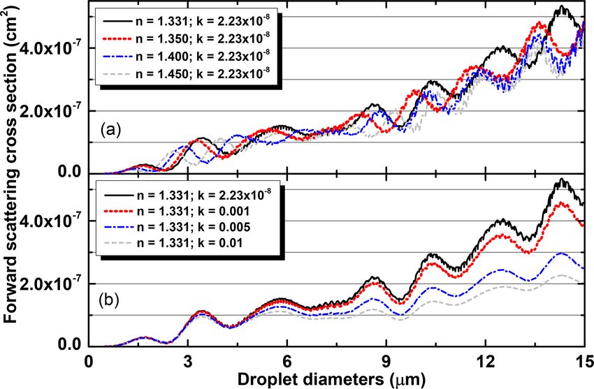
S. N. Vâjâiac et al.: Post-flight analysis of detailed size distributions                                                     6779

tive for the entire set of detected particles during a measure-     2   The detailed shape of the FWSCS-diameter diagram
ment session. This assumption is fundamental for our pro-
posed use of PbP data in detailed post-flight analyses.             According to Mie theory, the differential scattering cross sec-
   In the following sections we present a methodology for ob-       tion of light on dielectric spheres with given complex refrac-
taining detailed droplet size distributions from such PbP sam-      tive indices is a complicated function of both the scattering
ple files. This study relies on an analysis of a “most detailed”    angle and the diameters of the scatterers. The details of this
shape of the FWSCS-diameter diagram for pure water. As all          formalism can be found in any classic book on the subject
local “ripples” of this diagram may play a role in sizing cloud     (e.g., Bohren and Huffmann, 1983), so its derivation is omit-
droplets, it is concluded that the size distributions of various    ted in this paper. As the intensity of the scattered light can-
cloud parameters, as well as their bulk values, are most accu-      not be determined at a specific value of the scattering angle,
rately expressed in post-flight analyses by using “the finest”      any instrument used for such measurements is designed to
equidistant division (or mesh points) of the range of particle      capture the scattered light in a certain angular interval. The
diameters. Nevertheless, for certain purposes, droplet distri-      standard CAS collects the forward-scattered light. Therefore,
butions over coarser size grids (which are readily available        its sensors usually cover a small (around 10◦ ) angle near the
from the “basic” ones obtained over the finest set of equidis-      direction of the incident laser beam. It follows that the CAS
tant mesh points) may prove more practical. An obvious ex-          is actually measuring an integral of the differential scattering
ample is the design of unambiguous divisions of the whole           cross section over that specific angular interval. The value of
range of diameters into uneven size bins for use in in-flight       this integral is what we call the FWSCS. We mention here in
recordings. Also, coarser equidistant size grids can be very        passing that the FWSCS still retains a quite strong sensitivity
convenient in post-flight error evaluation of resulting cloud       on the limits of the collecting angular interval, especially on
parameters.                                                         its upper bound (Baumgardner et al., 2017), so the accurate
   The proposed methodology is illustrated on short (a few          knowledge of these constructive parameters is of utmost im-
minutes) selections of data recorded during previous mea-           portance for an objective use of the instrument. Our computa-
surement campaigns of water clouds with an airborne CAS             tions of the FWSCS have been performed through integration
instrument. Error assessment is also performed in detail for        over the fixed angular interval stretching from 4.0 to 13.5◦ .
the results obtained with the considered example data.              It is also worth mentioning here that the wavelength used in
   Additionally, some possible influences of atmospheric            FWSCS calculations was λ = 658 nm at which our instru-
aerosols on the outcomes of the CAS measurements are dis-           ment operates, according to its technical specifications. At
cussed, with emphasis on the possible alteration of the opti-       this wavelength, pure water is almost non-absorptive (more
cal properties of cloud droplets by the dissolving or the in-       precisely, the real and imaginary parts of the refractive index
clusion (starting from the nucleation step) of sub-micrometer       are n = 1.331 and k = 2.23 × 10⁻⁸ , respectively).
particles of hygroscopic or hydrophilic aerosol. The impor-            Turning now to the FWSCS-diameter diagram, any type
tance of the optical properties of measured particles has been      of CAS instrument determines the size of cloud particles
long addressed in the literature (Liu et al., 1974; Dye and         through comparison between measured and theoretical val-
Baumgardner, 1984; Baumgardner et al., 1992; Johnson and            ues of FWSCS, thus attempting an inversion of the FWSCS-
Osborne, 2011; Rosenberg et al., 2012; Granados-Muñoz et            diameter functional dependence. The characteristics of this
al., 2016). The wavelength of the light provided by a CAS           dependence are therefore of paramount importance in the nu-
light source is normally chosen in a range where pure water         merical phase of the CAS sizing process. Nevertheless, the
has virtually no absorption. The whole sizing procedure as-         theoretical FWSCS-diameter relationship is too complicated
sumes that any measured particle is a droplet of pure water,        to be cast in a closed analytical form and it should be cal-
and the FWSCS-diameter diagram, which is the basic com-             culated point by point for a certain set of diameter values.
parison tool, is constructed for the specific case of pure water.   As mentioned before, the typical range of diameters of par-
It follows that a significant increase in the absorption and/or     ticles detected by CAS is 0.5–50 µm. The FWSCS diagram
refractivity properties of “contaminated” cloud droplets may        can be computed within this fixed range, at a certain num-
induce drastic changes in their sizing from comparisons with        ber of equidistant mesh points, Nd . Constructing the FWSCS
the pure water diagram. These changes, if very numerous,            curve for increasing values of Nd uncovers more and more
may further degrade the objectivity of CAS measurements,            ripples of it, as illustrated in Fig. 1, which shows a closeup
the ensuing size distributions of cloud droplets and the values     of the dimensional range of scatterers between 37 and 40 µm.
of important bulk cloud properties. To improve the reliabil-        The figure’s main panel contains the corresponding segment
ity of such results, some complementary measurements are            of the FWSCS-diameter curve plotted for three increasing
suggested.                                                          values of Nd (and thus for three increasing densities of mesh
                                                                    points on the abscissa). It can be seen that, once Nd increases,
                                                                    the curves look increasingly oscillatory at the local level. The
                                                                    presence of ripples clearly constitutes a difficulty in the pro-
                                                                    cess of retrieving a particle’s size from a specific value of

https://doi.org/10.5194/amt-14-6777-2021                                              Atmos. Meas. Tech., 14, 6777–6794, 2021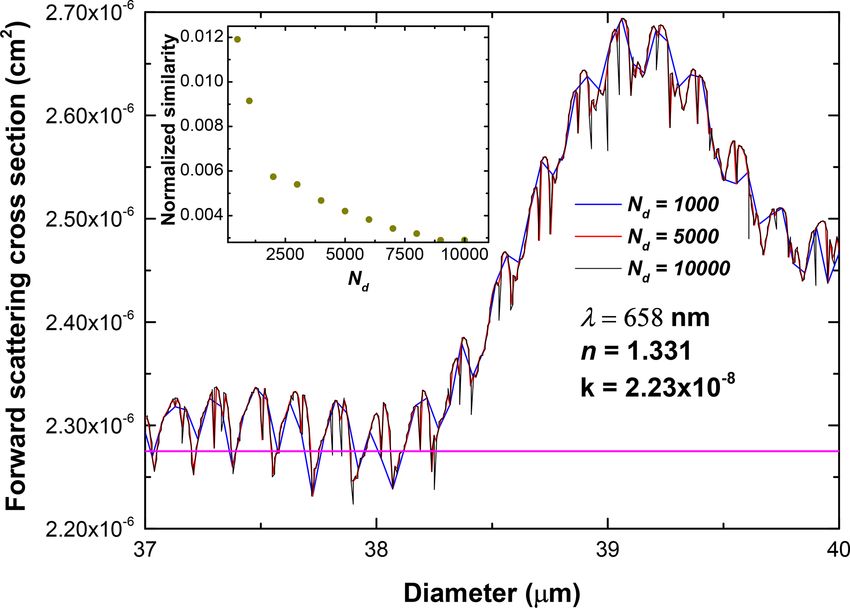
6780                                                          S. N. Vâjâiac et al.: Post-flight analysis of detailed size distributions

                                                                         found that, with increasing Nd , the shapes of the resulted di-
                                                                         agrams change and become more detailed and increasingly
                                                                         similar. In quantitative terms, the similarity of two such dia-
                                                                         grams can be measured by the area enclosed between them.
                                                                         For convenience, these areas have been normalized to the
                                                                         area under the finest plot in the sequence (namely that cor-
                                                                         responding to Nd = 10 000) and called “normalized similar-
                                                                         ities”. Thus, for each FWSCS plot in the sequence the nor-
                                                                         malized similarity with the preceding one in the sequence
                                                                         has been computed. The normalized similarities have then
                                                                         been represented against their Nd values, and the result is
                                                                         presented in the inset of Fig. 1. It can be seen that the dif-
                                                                         ference in shape between two successive FWSCS diagrams
                                                                         drops close to zero for over 9000 mesh points. As a conse-
                                                                         quence, a reference value of Nd = 10 000 equidistant mesh
Figure 1. Detail of the FWSCS vs. particle diameter diagram plot-
                                                                         points on the abscissa has been used in all following compu-
ted for three different values of the mesh point number, Nd , on the     tations.
abscissa (the blue, red and black lines on the main panel). The wave-
length of the radiation, λ, as well as the corresponding real (n) and
imaginary (k) parts of the refractive index of pure water are indi-      3   Retrieving particle diameters from the comparison
cated in the main panel. Increasing densities of these mesh points re-       with the FWSCS diagram
veal more rippling in the structure of the curve. This, in turn, makes
the particle sizing increasingly ambiguous. The pink horizontal line     As mentioned in the above discussions, the non-
corresponds to a single measured value of 2.275 × 10⁻⁶ cm2 which         monotonicity of the FWSCS-diameter dependence induces
intersects the FWSCS diagram multiple times. Thus, assigning a           an important difficulty when extracting a particle’s size
unique value for the diameter is impossible. The inset illustrates the
                                                                         from the FWSCS value it generates in a CAS instrument.
analysis of the shape convergence of the FWSCS plots for increas-
ing mesh point density on the abscissa.
                                                                         To be more precise, while there is an overall increase in
                                                                         the FWSCS values for larger scatterers, the dependence is
                                                                         quite oscillatory, and, at the local level, it shows a very noisy
                                                                         structure of small ripples. Therefore, as shown before in
the FWSCS. For example, when assuming a measured value                   Fig. 1, this makes the particle sizing highly ambiguous. A
of 2.275 × 10⁻⁶ cm2 (indicated by the pink horizontal line in            way to get around this difficulty would be to use a coarser
Fig. 1), there are multiple possible values for the diameter             and uneven partition of size bins over the whole measurable
of the scattering particle that produces such a response. That           range of particle diameters. As mentioned before, the bin
number is obtained by counting all of the intersections of the           limits should be designed unambiguously, in the sense
horizontal line in the FWSCS diagram. This number obvi-                  that the corresponding FWSCS thresholds have unique
ously increases when the diagram is computed in greater de-              intersections with the diagram. For practical purposes,
tail. This aspect, which generates sizing ambiguities through            partitions of the diameters’ range in uneven size bins have
FWSCS measurements, has been known and analyzed for a                    been previously proposed in the literature (Pinnick et al.,
long time in the literature (Pinnick et al., 1981; Baumgardner           1981; Dye and Baumgardner, 1984). Such procedures are
et al., 1992; Brenguier et al., 1998). More recent studies on            actually fitting of the exact FWSCS-diameter diagram with
OPCs (Rosenberg et al., 2012) consider in greater detail the             a discrete monotonic plot of response thresholds, each
consequences of the non-monotonicity of the FWSCS vs. di-                corresponding to a size bin limit. The fitting should be made
ameter correspondence but focus mainly on the issues related             so that the differences between the threshold plot and the
to the instrument calibration.                                           exact Mie diagram can be assimilated to the resultant of
   There is an obvious practical question that arises in con-            the various errors generated in the FWSCS measurement
nection to the local irregularities of the FWSCS curve: how              process (Brenguier et al., 1998; Granados-Muñoz et al.
fine should the division of points on the abscissa be to re-             2016).
veal all the local features of its size dependence? In other                Due to the high density of ripples in the FWSCS curve,
words, one should settle on a sufficiently large value of the            the possibilities of constructing strictly unequivocal (but still
number Nd in order to have a reliable theoretical FWSCS-                 meaningful) divisions of bins are limited (but not unique).
diameter diagram that displays the full “noisiness” of this de-          This fact may become a problem when there is an interest
pendence. In order to answer this problem, the diagram has               in detailing regions of the cloud droplets’ dimensional spec-
been computed in the same range of diameters (0.5–50 µm),                trum, which fall in the noisiest parts of the FWSCS diagram.
for an increasing sequence of mesh point numbers. It was                 A straightforward possibility to overcome this hurdle would

Atmos. Meas. Tech., 14, 6777–6794, 2021                                                   https://doi.org/10.5194/amt-14-6777-2021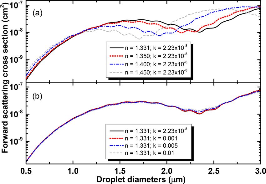
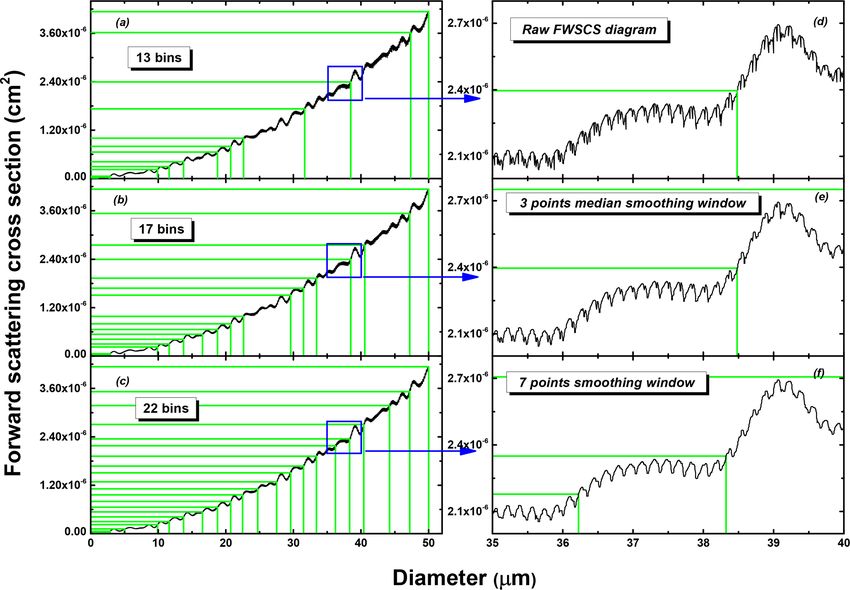
S. N. Vâjâiac et al.: Post-flight analysis of detailed size distributions                                                             6781

Figure 2. Size and FWSCS bin structures induced on the FWSCS-diameter diagram. Green lines in panels (a), (b) and (c) indicate the size
bins (on the abscissa) and the FWSCS bins (on the ordinate), for three degrees of smoothness, as indicated in panels (d), (e) and (f), where
one same detail of the diagram is magnified for clarity.

be to use various smoothed versions of the FWSCS-diameter               then the bin was merged with its next adjacent neighbor).
diagram. Numerical smoothing of a dataset can be achieved               In this way, a one-to-one correspondence is established be-
in several ways, but only the resulting shape is relevant. The          tween the FWSCS thresholds and the limits of the size bins.
smoothing should be performed in a balanced degree, such                It should be noted that certain maximal bins can be split in
that it does not alter the main features of the functional de-          smaller (but relevant) ones, with unequivocal limits. Figure 2
pendence described by the diagram.                                      illustrates how the degree of smoothing of the FWSCS dia-
   An illustration of this requirement is presented in Fig. 2.          gram influences the bin width and spacing. When applying
Here we consider three versions of the FWSCS diagram and                the bin construction method to the raw FWSCS diagram, a
select the maximum number of bins for each of them. The                 number of 13 maximal bins is obtained (shown in Fig. 2a and
first diagram (Fig. 2a) is the “raw” FWSCS curve (com-                  detailed in Fig. 2d), which can be too coarse, especially for
puted at 10 000 mesh points on the abscissa), and the other             obtaining meaningful information about particles of larger
two (Fig. 2b, c) are smoothed versions of it constructed by             sizes.
the so-called median smoothing method which averages the                   By applying a three-point smoothing window, the number
FWSCS values at a certain (odd) number of consecutive                   of maximal bins increases to 17 (Fig. 2b and e). Moreover, if
points on the abscissa. The number of points over which the             the smoothing window is increased to seven points, the num-
average is performed is called the smoothing window. The                ber of maximal bins becomes more representative across the
maximal bin configuration has been established for each case            entire measurable particle range (22 in Fig. 2c), and more de-
according to two constraints. First, as already mentioned, it           tailed information about the larger particles is retained. This
was required that the horizontal lines drawn for each FWSCS             improvement, however, is obviously obtained at the expense
threshold intersect the diagram at a single point. The second           of distorting the local structure of the FWSCS-diameter dia-
requirement was that the width of a size bin was not irrele-            gram (Fig. 2f). If the degree of smoothing is pushed further,
vantly small (for example, if the width of a size bin turned out        even larger-amplitude undulations of the curve are wiped out,
to be lower than 5 % of the value assigned to its upper limit,          and its deviation from the raw diagram is enhanced.

https://doi.org/10.5194/amt-14-6777-2021                                                   Atmos. Meas. Tech., 14, 6777–6794, 2021
6782                                                      S. N. Vâjâiac et al.: Post-flight analysis of detailed size distributions

   The splitting of the range of cloud particle diameters into       tersections of the measured value with the FWSCS diagram),
relatively large and uneven size bins is clearly very helpful        each one of which is a possible optical diameter of the parti-
in practical in situ measurements as it both allows for rapid        cle that produced the measured FWSCS response. As we lack
in-flight counting and sizing of cloud particles and saves stor-     information on which of these alternatives is more probable,
age memory by generating relatively small data files. The            we are forced to assume that any of them is equally possi-
process of generating the size bin structure automatically           ble. In other words, given the measured value of the FWSCS,
produces the corresponding FWSCS grid of maximal bins,               we count n10 for each diameter where the computed diagram
which can eventually be supplemented with smaller unam-              takes on that value. In this way, we replace integer particle
biguous divisions. This technique, in principle, allows for the      counts in unequivocal (but large and uneven) size bins with
rapid sizing of every valid particle that was sampled by the         fractional particle counts associated with each mesh point of
instrument, with no need to retain the particular value of the       the dense, equidistant grid of diameters. Detailed pointwise
FWSCS it produced. The resulting statistics are usually ex-          size distributions can thus be constructed. They can be used
pressed in various histograms (normalized or not) over the           as they are but can also be grouped in any structure of bins,
pre-established structure of size bins. Nevertheless, the prac-      including that resulting from the smoothing of the FWSCS
tical procedure is not so simple as the FWSCS of a particle          diagram, as described in the preceding section. The most im-
is quantified in voltage counts of some specialized sensors          portant advantage of the proposed approach is that, instead of
(Baumgardner et al., 2001). Thus, the theoretical FWSCS              an uneven grid of size bins, one may use a structure of a con-
grid of thresholds must be made to correspond to a grid of           venient number of equal size bins (e.g., 1 µm wide). In most
threshold counts of the sensor. This process involves precise        situations, when presented in this way, the size distribution
knowledge of some electronic parameters of the instrument            retains its information across all measurable sizes.
(since generating the voltage signals usually requires differ-          As already stated, the PbP output files contain detailed
ent non-linear amplification stages) and of certain specific         records on a certain subset of the entire group of measured
constructive parameters of the instrument (like the angular          particles in a given flight segment. The particles that en-
collecting range of the scattered light, the effective sample        ter the instrument during a flight segment and qualify for
area, the laser wavelength and the cross-sectional inhomo-           FWSCS measurement are normally so numerous that they
geneity of its beam). Therefore, it is expected that construct-      can be treated as a statistical ensemble. The particles of
ing the sequence of threshold voltage counts to be associated        which FWSCS values have been recorded in the PbP files
with the size bin structure brings a certain amount of error         are selected only on their arrival time in the sample volume
that (in some cases, especially for older versions of such in-       of the CAS. As for the selection of these particles, no size
struments) may be difficult to evaluate. Due to these difficul-      criterion has been imposed (except for that of fitting into the
ties, the rapid in-flight statistical analysis of cloud particles    0.5–50 µm measuring range of the instrument), and it follows
should be complemented, whenever PbP FWSCS recordings                that their sets will bear the same size statistical specifics as
are available, with post-flight PbP analysis.                        the entire ensemble. These size statistical peculiarities may
                                                                     include eventual dimensional gaps that can occur due to var-
                                                                     ious effects, e.g., cloud mixing (Beals et al., 2015). This ob-
4   Expressing cloud particle statistics from PbP files by           servation is key in acknowledging the usefulness of the PbP
    using a fine grid of particle diameter values                    data. As noted in this section, detailed, pointwise size distri-
                                                                     butions can be obtained from the PbP output files. By further
As discussed in the previous section, while rapid and mem-           grouping these distributions over the very (uneven) bin struc-
ory saving, the use of uneven size bin structures constructed        ture that served for the in-flight bulk data recording, one may
from the unequivocalness requirement inherently lose impor-          compare the ensuing size distribution with that provided by
tant details about the particle size distributions, especially at    the instrument (if both are properly normalized, for example
larger sizes (where the FWSCS diagram is more rippled).              at the total number of particles in each recording). If consis-
These ensuing errors are critical when size distributions are        tent, the PbP sample data should generate size distributions
used to derive quantities that are highly sensitive to larger        similar to those produced by the bulk data file. Such consis-
particles like the liquid water content (LWC). To overcome           tency checks of the PbP files can be easily performed for each
such drawbacks, we propose the use of a dense mesh of a              sequence of data to be processed through post-flight analysis
convenient number of equal size bins. This number of bins            in order to remove eventual accidental artifacts.
could be as large as that of the number of mesh points on               In this connection, we note that the statistical consistency
the abscissa (10 000) for which the shape of the FWSCS-              of the PbP data might be questioned due to the fact that the
diameter diagram stabilizes, as discussed in Sect. 2. Fur-           corresponding particles are not randomly picked from the
ther, consider a certain measured value of the FWSCS (i.e.,          set detected in the whole sampling instance. They are the
a given entry of the PbP file). When theoretically comput-           first ∼ 290 in this set, and one may suspect that this very
ing the FWSCS, the same value is obtained for a number of            choice might induce a statistical bias. However, when com-
values, n0 , of the particle diameter (they correspond to all in-    bining many consecutive sampling instances, one can expect

Atmos. Meas. Tech., 14, 6777–6794, 2021                                               https://doi.org/10.5194/amt-14-6777-2021
S. N. Vâjâiac et al.: Post-flight analysis of detailed size distributions                                                                 6783

Figure 3. Number (a, b) and LWC (c, d) size distributions obtained from the post-flight analysis of PbP data recorded during a flight line
performed on 26 September 2019, over some area of Romania. The diagrams (a) and (c) are detailed distributions and show a fine structure
of size modes, which are “wiped” out if spread over coarser size grids, as seen on the histograms (b) and (d) constructed over a structure of
50 equal size bins. Nevertheless, these coarser representations allow for sufficient resolution to accurately compute various averages and are
more convenient in evaluating maximal relative errors, as described in the next section. Note the unusual range of LWC values due to the
small amounts of liquid water counted in each division of the very fine grid of diameter values. Also, in panel (d), note that the levels of the
LWC distribution are higher than those of panel (c) as they collect the contributions of particles from larger divisions of diameter values.

that the statistical bias (if any) is effectively eliminated and          particles are detected in the instrument (the sample area, as
that the PbP data behave statistically in a similar way as the            will be further discussed in Sect. 5). By contrast, the sam-
bulk data file. There is a further related question could: how            ple volume of the set of particles that generate the PbP file
many sampling instances are necessary to achieve statistical              (denoted simply by Vs ) is more difficult to retrieve since the
consistency of the PbP data? The answer would clearly de-                 selection of these particles is not continuous along the flight
pend on the density of the droplet population in the given                segment. By assuming that the total set of particles measured
flight segment. The denser the corresponding cloud area, the              in a flight segment and the selected subset that generates the
longer the recording should be in order to achieve a statisti-            PbP file have similar statistical behaviors, one may compare
cally consistent PbP data file. In general, by assuming that in           their related size distributions over the uneven bin structure
a sampling instance the instrument can measure enough par-                used for the in-flight bulk data recording. Using the nor-
ticles to produce a significant distribution, we conjecture that          malization of these distributions at the corresponding sam-
the total length of the PbP data file should be at least equal            ple volumes, their shapes should be, in principle, identical.
to the average number of qualified particles during a single              At this point, one can use Vs as an adjustable parameter and
sampling instance.                                                        compute its value from the condition that the “distance” be-
   If normalized to the so-called sample volume of each                   tween the two distributions (defined as the root mean square
recording, further information can be very conveniently re-               of their bin differences) is at a minimum. The accuracy of
trieved from the comparison of the aforementioned size dis-               this procedure can be further improved by using LWC size
tributions. The sample volume of some recording is the to-                distributions (also normalized at the corresponding sample
tal volume of air that is transiting the instrument during that           volumes) instead of number size distributions. The size dis-
particular recording. For the bulk data of a certain flight seg-          tribution of the LWC over the uneven bin structure used in
ment, the sample volume (to be denoted by Vstot ) can be de-              the rapid in-flight measurements is readily obtainable from
termined quite easily as the product of the total duration of             the corresponding number size distributions by multiplying
the flight line, the air speed and the physical area in which             it with the central water droplet mass of each size bin (i.e.,

https://doi.org/10.5194/amt-14-6777-2021                                                      Atmos. Meas. Tech., 14, 6777–6794, 2021
6784                                                         S. N. Vâjâiac et al.: Post-flight analysis of detailed size distributions

                                                                        50 µm, which is the measuring range of our instrument. The
                                                                        significant parts of the number and LWC size distributions
                                                                        are shown in panels (a) and (c) of Fig. 3. The most striking
                                                                        aspect related to these diagrams is the display of fine struc-
                                                                        tures showing certain dimensional preferences (or “modes”)
                                                                        of the cloud droplets. Highlighting such peculiarities by in
                                                                        situ measurements might prove useful for correlating cloud
                                                                        microstructure with the properties of the aerosol particles that
                                                                        are present in the studied area (as long suggested in the lit-
                                                                        erature – e.g., Squires, 1952; Mordy, 1959; Sorjamaa et al.,
                                                                        2004) as well as other cloud microphysical processes.
                                                                           Such detailed analysis of in situ collected data could not
                                                                        be possible if the distributions were constructed over coarser
                                                                        size bins. This point is illustrated in panels (b) and (d) of
                                                                        Fig. 3, where the same statistics as those presented in pan-
                                                                        els (a) and (c) have been built over an equidistant grid of bins,
                                                                        each of almost 1 µm in length. This grid is almost 200 times
Figure 4. Droplet size distribution of Fig. 3a and b (panels a and
b, respectively) shown in comparison with the size distribution of      coarser than the detailed one but still preserves some major
the same droplets constructed over the 30-bin structure used for the    features of the two distributions. By contrast, the usual CAS
in-flight data acquisition.                                             acquisition software allows for only 30 (uneven) size bins
                                                                        where the probed particles can be distributed. It is obviously
                                                                        expected that such coarse grids may further smoothen the
                                                                        detailed shapes of the distributions, and this aspect is made
the mass of a spherical water droplet with the diameter equal           particularly clear by examining the plots of Fig. 4. Here, in
to the median of the bin).                                              panels (a) and (b), the detailed and the 50 equal size bin
   The aforementioned methodology has been applied to                   distributions have been reproduced from Fig. 3a and b, re-
some data recorded by our group during recent measure-                  spectively. For comparison, the plot of Fig. 4c shows the size
ment campaigns. Our instrument, a CAS with depolarization               distribution from the same PbP file, but represented over the
(CAPS-DPOL) produced by Droplet Measurement Tech-                       30 bins structure used for the in-flight data acquisition. Due
nologies Inc. (DMT), in 2011, is mounted on a Beechcraft                to the small widths of the bins in the sub-micrometer range,
C90GTx aircraft. The data files are usually quite large, but            the distribution of Fig. 4c has some resemblance to the de-
the post-flight analysis has mainly focused on selected seg-            tailed one of Fig. 4a, in the same region. However, between 8
ments where the aircraft flew in warm clouds at approx-                 and 20 µm (a particularly important size range for the micro-
imately constant altitudes, thus probing various horizontal             physics of warm clouds), the 30-bin distribution looks rather
transects of the cloud. Such segments are hereafter referred            “dull” and clearly lacks the structural richness of the repre-
to as flight lines. To illustrate the typical post-flight analysis      sentation shown in Fig. 4a. Nevertheless, as already pointed
that we performed with our recorded data, a single example              out before, coarser bin structures allow rapid in-flight pro-
will be discussed in this section. The data were collected in           cessing, use shorter data files and may serve for validating
a flight line during a measurement campaign performed in                the PbP recordings as well as for computing specific func-
September and October 2019, over Romania. A further ex-                 tional parameters.
ample is additionally used in the next section and refers to               As a conclusion, using the PbP data files, the methodology
similar measurements performed in April 2019. A compre-                 described in this section allows the construction of detailed
hensive description and discussion of these campaigns will              size distributions of cloud droplets if accurate descriptions
follow in a forthcoming paper. The PbP file contains de-                are needed. Such a procedure may be useful, for example,
tailed values of the measured FWSCS detector counts for                 in precise instrument calibrations (Rosenberg et al., 2012).
71 014 particles, which represent an excerpt of the total num-          Coarser size distributions (over equal or uneven bin struc-
ber of particles that were validated and classified amongst a           tures) are also readily available from the detailed one, for use
predefined size bin structure. According to the DMT proce-              in computing various cloud microphysical parameters.
dures, the result of this classification is recorded in a separate
output file without retaining any specifics for individual par-
ticles.                                                                 5   General expression of cloud microphysical
   Applying the recipe described in this section to the PbP                 parameters and the ensuing errors
data recorded in the example flight line, the related detailed
size distributions are constructed over a typical fine grid of          Mathematical expressions for microphysical quantities of
10 000 values for the particle diameters, between 0.5 and               clouds (like droplet effective diameter or LWC) usually con-

Atmos. Meas. Tech., 14, 6777–6794, 2021                                                  https://doi.org/10.5194/amt-14-6777-2021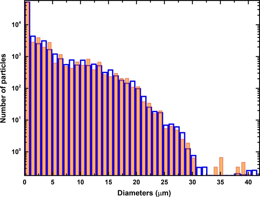
S. N. Vâjâiac et al.: Post-flight analysis of detailed size distributions 6785
tain various averages over the size distributions of droplets. Along with computations of bulk quantities of the type de-
Each such average implies a summation over the values taken fined generically in Eq. (1), it is also necessary to evaluate
by a certain function of droplets’ diameters, y(d). The sum the related error interval or, equivalently, the absolute error
(whose value we denote by Y ) can generally be written as δ(Y ). A natural and reliable approach would be to first com-
pute the relative error of the quantity Y :
Zdm
Y = y (x) c (x) dx, (1) δ (Y )
ε (Y ) = . (5)
d0 |Y |
where c(x)dx is the number of particles detected in the diam- As the error analysis is simpler in continuous variables, we
eter interval (x, x + dx) per unit of explored volume (the so- return to Eq. (1), which can be more conveniently detailed in
called number concentration of particles). The integration is the following form:
over the maximal interval (d0 , dm ) within which the particle
diameters can take values (in our case, it is the measurement Zdm
range of the instrument, namely d0 = 0.5 and dm = 50 µm). 1
Y= y (x) N (x) dx, (6)
For example, to obtain the LWC, the function y(x) in Eq. (1) Vs
d0
should be replaced by some constant multiple of x 3 . Also,
for computing the extinction coefficient from its practical ex- where N (x)dx is the number of detected particles having the
pression (approximated as twice the optical cross section for diameters in the range (x, x + dx). The error in Y originates
cloud droplets and visible wavelengths – see, for example, partly in the imprecision of determining the sample volume
Kokhanovsky, 2004), y(x) in the integrand of Eq. (1) should Vs . The other source of ε(Y ) originates in the error of each
be x 2 . For computing the effective diameter (def ) of droplets, measured value of the FWSCS, which translates in a com-
one should consider a more complicated expression involv- plex way to the number distribution N (x). When assuming
ing a ratio of two integrals of the type shown in Eq. (1): one such an imprecision for the FWSCS optical measurements,
with y(x) = x 3 divided by the other with y(x) = x 2 . Never- the distribution N (x) takes another shape and shifts to a new
theless, the following discussions essentially apply for this function denoted by Ñ (x). The shift between these two dis-
case too. tributions should have no constant sign over the whole range
Equation (1) is written in the assumption that the number of diameters. On the contrary, their difference should oscil-
concentration is known for every value of the diameter. How- late around zero as any overestimation of the particle num-
ever, as already discussed, all practical size distributions are ber in a certain size range should induce an underestimation
discrete functions, over some finite number of bins (evenly, somewhere else. We can therefore write
or unevenly spaced), to be denoted by Nb . In passing, we !
may note that Nb should not exceed the total number of mesh dRm
points, Nd , on the abscissa where the detailed FWSCS dia- δ y (x) N (x) dx
d0
gram was computed. For such discrete distributions, the in- ε (Y ) = ε (Vs ) + . (7)
dRm
tegral in Eq. (1) can be approximated by the corresponding
y (x) N (x) dx
sum over these bins: d0
Nb
X
Y= y (di ) ci , (2) Moreover,
i=1
where di and ci are the representative diameter (e.g., the me- Zdm Zdm h i
δ y (x) N (x) dx = y (x) Ñ (x) − N (x) dx . (8)
dian) of the size bin number i and the number concentration
of particles found in that bin, respectively. At this point, it d0 d0
is useful to explicitly detail ci by using the value of the sam-
ple volume, Vs , which can be obtained through the procedure Thus,
described in the previous section. Thus, we should write
dRm h i
Ni y (x) Ñ (x) − N (x) dx
ci = , (3) d0
Vs ε (Y ) = ε (Vs ) + . (9)
dRm
where Ni is the total number of particles detected in the ith y (x) N (x) dx
bin (the sequence of all these numbers represents what is usu- d0
ally called the number distribution of particles over the given
size bins). Therefore, Eq. (2) becomes As already discussed, integrals like those appearing in Eq. (9)
Nb
can be practically computed by summing over some custom
1 X grid of size bins. If the grid were made of uneven bins, then
Y= y (di ) Ni . (4)
Vs i=1 the errors ensuing from the eventual smoothing procedure of
https://doi.org/10.5194/amt-14-6777-2021 Atmos. Meas. Tech., 14, 6777–6794, 20216786 S. N. Vâjâiac et al.: Post-flight analysis of detailed size distributions
the FWSCS diagram (which, in some cases, could be quite
consistent) should also be taken into account. To avoid such
artificial extension of the overall imprecision, a grid of equal
bins (which is defined, so it is not affected by errors) is nor-
mally recommended. Using such discretization of the range
of diameters in equal bins, one obtains
Nb
P
y (di ) Ñi − Ni
i=1
ε (Y ) = ε (Vs ) + . (10)
Nb
P
y (di ) Ni
i=1
For the case of def which can be computed through the rela-
tion
Nb
P
Ni di3 Figure 5. Detail of the FWSCS-diameter diagram showing a mea-
i=1 sured value, C (red line), of a particle’s FWSCS and the ensuing er-
def = , (11) ror strip (yellow region). The particle’s contribution to the distorted
Nb
Ni di2
P
size distribution can be computed by considering the “length” of the
i=1 “blurred” intersection of the error strip with the FWSCS diagram.
That length, 8err , is defined as the absolute values of the sum of
the relative error takes a form that is independent of the im- the ordinate projections of all the monotonic parts of the diagram
precision in Vs : that fit within the error strip. If we further restrict to the part of the
curve that fits within the error strip and in the size bin #i, then the
Nb Nb
analogous length 8ierr results. Its ratio to 8err is the weight with
Ñi − Ni di3 Ñi − Ni di2
P P
i=1 i=1 which the given particle contributes to the size bin #i (enclosed by
ε (def ) = + , (12) the vertical green lines).
Nb Nb
Ni di3 Ni di2
P P
i=1 i=1
that the true value can be found, with uniform probability,
where Ñi is the “distorted” distribution of particles over bins. somewhere in the horizontal strip defined by the interval
In this way, the remaining problem is to obtain Ñi as
h i
1 1
C − 2 δC, C + 2 δC in Fig. 5. In other words, instead of
generated by the error associated with each experimental
FWSCS. At this point, it should be mentioned that the in- obtaining a sharp, exact value C for the FWSCS, the instru-
fluence of the sizing errors on the resulting droplet distribu- ment provides a blurred figure of width δC. It is obvious that
tions has been previously addressed in detail in the literature the wider the error strip for C is, the larger the imprecision
(Cooper, 1981; Baumgardner et al., 1992; Brenguier et al., of the particle sizing will be. For this reason, it is further
1998) through an ingenious mathematical method based on assumed that the maximal distortion of the size distribution
a transfer matrix that takes the measured distribution into the from the one obtained with exact values of the FWSCS re-
actual one. The elements of the matrix are actually probabil- sults by counting the blurred intersections of the FWSCS-
ities that a certain measured particle of a given diameter be diameter diagram with the error strips associated with each
counted in a different size bin. The transfer matrix has to be measured particle. To proceed in this computation, consider
constructed for each instrument, and its elements embed both first the intersection of the horizontal line at C− 12 δC with the
the errors generated by the FWSCS measurements and those FWSCS diagram. Let the abscissa of that point be denoted by
ensuing from the ambiguities in the comparison with the Mie dmin . Also, name dmax the abscissa of the rightmost intersec-
diagram. tion of the horizontal line at C + 21 δC. As clearly illustrated
The present study tries a different approach, by separating in Fig. 5, not all the points of the FWSCS diagram with ab-
the measurement errors of the FWSCS values (which stem scissae between dmin and dmax fall within the error strip (for
from various hardware issues and have to be known) and by example, points with d around 40 µm are not included). Now,
considering in greater detail the uncertainties generated by imagine that we remove from the interval [dmin , dmax ] all the
the comparison with the “exact” Mie diagram. abscissae for which the FWSCS values fall outside the error
To make any meaningful progress in this approach, one strip. The remaining set, which is actually a union of smaller
should actually resort to evaluating the related maximal dis- intervals, will be called 1. As the true value of the measured
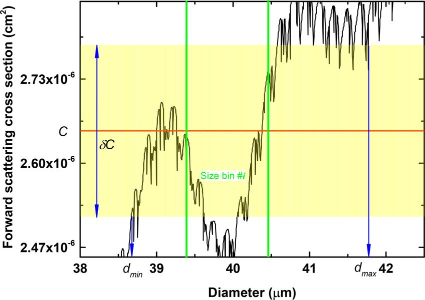
tortion error. Such an attempt could be imagined as follows. FWSCS is assumed toh be somewhere in thei (yellow) strip
For any measured value, C, of the FWSCS, there should defined by the interval C − 12 δC, C + 12 δC , it is clear that
be an assumed absolute error, δC. We will also assume the true value of the particle’s diameter associated with the
Atmos. Meas. Tech., 14, 6777–6794, 2021 https://doi.org/10.5194/amt-14-6777-2021S. N. Vâjâiac et al.: Post-flight analysis of detailed size distributions 6787
value C of the FWSCS should lie within the set 1. Accord-
ing to our assumption,
h every value ofi the FWSCS within the
error interval C − 12 δC, C + 21 δC has the same chance of
being the true one. On the other hand, every horizontal line
drawn within the error strip will intersect the FWSCS in a
unique set of points, with a unique set of abscissae. However,
from one horizontal line to another, the number of intersec-
tions may differ (depending on the local shape of the FWSCS
diagram), so there should be different chances that one point
or another from the portion of the FWSCS within the error
strip corresponds to the true diameter. The same should be
valid for the corresponding weights with which the particles’
diameters enter in the counting of each size bin. To quantify
the weight for a given size bin, one might select from the
set of all intersection points of the FWSCS diagram with the
error strip only the set of points whose abscissae fall inside
that size bin. Then, the required weight will be the ratio of the Figure 6. Nominal (orange) and distorted (hollow blue) number dis-
measures of these two sets of points of the FWSCS diagram, tributions over a structure of 50 equal size bins. The distorted his-
namely the smaller one to the larger one. Unfortunately, the togram is obtained with the assumption that FWSCS measurements
have a homogeneous overall error of 10 % from the nominal values.
usual representations of the FWSCS curves are not metric
spaces, so one cannot simply use the length of the curve as
a measure of a set of its points. Instead, one could rely on Nb
P Nb
P
the “ordinate length” of a certain segment of the curve. This y (di ) Ñi − Ni ≥ y (di ) Ñi − Ni is formally cor-
quantity can be defined as the sum of the absolute values of i=1 i=1
the ordinate projections of all monotonic parts of the curve rect, its left term would lead to a physically overrated upper
within that segment. Thus, we can denote by 8err the ordi- bound of the error.
nate length of the portion from the FWSCS diagram that fits By attempting to apply the above recipe for error evalua-
within the error strip and by 8ierr the ordinate length of the tion to a too detailed distribution (as are the examples shown
subset of the diagram that fits within the error strip and has in panels (a) and (c) of Fig. 3), one may readily conclude
the abscissa projections within the size bin number i. The de- that the computational effort is inconveniently large, as usu-
sired weight with which the given particle contributes to that ally the analysis extends over multiple flight lines.
size bin can then be defined as the ratio 8ierr /8err . More- As pointed out in this section, one of the most difficult
over, by summing up these weights for all measured parti- task in error evaluation is computing the maximally distorted
cles, one can obtain the distorted number of droplets with size distribution. On the example flight line used in Sect. 4,
sizes contained in the bin number i, Ñi . As the distribution the distortion has been computed for the distribution over the
Ñi , obtained in this way, accounts for the maximal impre- equidistant structure of 50 bins. The result is plotted as a his-
cision of each FWSCS measurement, we assert that it rep- togram in Fig. 6, together with the exact (or “nominal”) dis-
resents the maximal departure from the “correct” distribu- tribution (the same as that appearing in Fig. 3b) for compar-
tion Ni . If replaced in Eq. (10), it will provide the maximal ison. One should note that the differences between the two
relative error of the quantity Y . Increasing the upper bound distributions may be locally quite large, although the log-
Nb
P arithmic scale of the ordinate might diminish their appear-
of the error by using the inequality y (di ) Ñi − Ni ≥ ance. The distorted distribution has been evaluated with the
i=1 hypothesis that FWSCS measurements bear a homogeneous
Nb
overall error of 10 % from the nominal values, which, for
P
y (di ) Ñi − Ni at the numerator of the second term
i=1 our instrument, is well below the manufacturer’s estimations.
of Eq. (10) would mean accepting the exceptional possibility Nevertheless, the errors in FWSCS measurements (more pre-
Nb
P cisely in the numbers of “counts” given by instrument’s de-
that the terms of the sum y (di ) Ñi − Ni are all posi- tectors at each measurement) may actually depend on various
i=1
tive. However, in the case of number distributions, this situa- conditions (e.g., on the gain stages used in a given measure-
tion can never happen due to the condition that the total num- ment) and cannot be taken as fixed at, say, 10 %. To evaluate
ber of particles is the same, irrespective of the way they are the impact of the accuracy in FWSCS measurements over the
Nb
P Nb
P imprecisions in the final values of the bulk parameters of the
distributed over the bins: Ñi = Ni . Thus, some terms clouds, we computed the ensuing relative errors induced in
i=1 i=1 three such quantities (namely the LWC, the extinction coef-
are necessarily negative, and therefore, while the inequality
ficient and the effective diameter) for a range of values of
https://doi.org/10.5194/amt-14-6777-2021 Atmos. Meas. Tech., 14, 6777–6794, 20216788 S. N. Vâjâiac et al.: Post-flight analysis of detailed size distributions
vals (sampling instances, e.g., 1 s each). Moreover, another
string of the bulk data file generated in-flight from all vali-
dated particles provides the final moments of each sampling
instance and is called “End Seconds”. These entries can be
used to extract the exact durations of the sampling instances
for the whole bulk recording. By multiplying these time in-
tervals with the corresponding PAS values and with the as-
sumed value of the sampling area, one readily obtains a string
of sampling volumes to be associated with the corresponding
sampling instances and, by summing them up, the flight line
sample volume, Vstot , is obtained. Due to the large impreci-
sion in the knowledge of the sample area (Lance et al., 2010),
the relative error of Vstot has been settled at the (generic)
value of 20 % in all cases considered in this study.
It should be noted here that, in principle, Vs could result
from a string of the PbP output file which records the time
Figure 7. Relative errors of the LWC, the extinction coefficient and separations between successive particle measurements (the
the effective diameter as functions of the relative error in measuring so called “inter-arrival particle time”, or IPT). However, as
the FWSCS. Different scales have been used on the axes in order to already mentioned, the PbP data are recorded only for the
reach a convenient aspect ratio of the figure. first ∼ 290 particles detected in a sampling instance, and the
IPT is retained for each measured particle, without count-
ing the “jumps” between successive sampling instances. This
the relative errors in measuring the FWSCS. It can be seen particular feature actually hinders the use of the IPT data
in Fig. 7 that, as expected, the increase in the imprecision string for reliably computing Vs and underscores the utility
for FWSCS makes the errors of all bulk cloud parameters and simplicity of the method described in Sect. 4.
grow. It is also remarkable that, while the generic range of Overall, we can conclude that evaluating the accuracy of
the relative errors of the FWSCS measurements is relatively cloud microphysical parameters obtained from CAS mea-
wide, some cloud parameters (like the extinction coefficient surements is no straightforward matter. It involves a compli-
or the effective diameter) tend to be determined with better cated and time-consuming analysis of the PbP files and re-
final accuracy through this methodology (at least over some lies on the knowledge of the detecting precision of CAS for
ranges) than that provided for the measured FWSCS values. individual particles, as well as on the precise knowledge of
According to the above discussions in this section, to com- constructive parameters of the instrument (e.g., the effective
pute relative errors of LWC and extinction coefficient one sample area).
needs to evaluate the relative error in the value of the sample
volume for the particles involved in the PbP recording, Vs .
Therefore, there will always be a background error for such 6 The effects of increased droplets’ refractivity and/or
bulk parameters. absorption on their sizing
In Sect. 4 we described a simple and reliable procedure
As discussed in the previous sections, due to the complicated
of obtaining Vs by comparing PbP vs. bulk data size distri-
shape of the FWSCS vs. diameter diagram, which is at the
butions over the operational in-flight structure of size bins.
core of the numerical phase of the CAS method, the whole
From this method, Vs results as a certain fraction of Vstot .
procedure of sizing cloud particles is far from straightfor-
Therefore, the relative error of Vs should be the sum of the
ward. Additional uncertainties may also stem from the as-
relative errors of Vstot and of the fraction itself. The fraction
sumption that the measured particles are pure water droplets.
error essentially stems from a comparison between the two
In fact, real cloud droplets are necessarily “contaminated”
size distributions, and it will be assumed negligible. Conse-
by aerosol particles, either by incorporating or by dissolv-
quently, the relative error of Vs will be taken as that of the
ing them (or even both), and it might be suspected that the
sample volume of the whole recording in the given flight
forward-scattered light from such complex particles might
line, Vstot . This parameter is actually a composite one, as it
differ from the case of pure water droplets of the same size. A
requires the knowledge of the velocity of the airflow in the
convenient approach to describe the optical response of con-
instrument (the so-called probe air speed, or PAS), the du-
taminated particles is by using a composite refractive index,
ration of the measurements and the so-called sample area,
which is generally larger (in both its real and imaginary parts)
which is the physical area where particles are detected. This
than the one of pure water (Erlick, 2006; Liu and Daum,
last quantity should be, usually, provided by the manufac-
2002; Liu et al., 2002; Wang and Sum, 2012; Mishchenko
turer. The output files constructed by the processing software
et al., 2014).
of CAS-DPOL typically provide the PAS at fixed time inter-
Atmos. Meas. Tech., 14, 6777–6794, 2021 https://doi.org/10.5194/amt-14-6777-2021You can also read