RainCast: A Rapid Update Rainfall Forecasting System for New Zealand

RainCast: A Rapid Update Rainfall Forecasting
System for New Zealand
Sijin Zhang (  zsjzyhzp@gmail.com )
 New Zealand Meteorological Service https://orcid.org/0000-0002-3456-8628
Gerard Barrow
 New Zealand Meteorological Service
Iman Soltanzadeh
 New Zealand Meteorological Service
Graham Rye
 New Zealand Meteorological Service
Yizhe Zhan
 New Zealand Meteorological Service
Chris Webster
 New Zealand Meteorological Service
Chris Noble
 New Zealand Meteorological Service

Research Article

Keywords: rainfall, nowcasting, NWP, seamless prediction

Posted Date: November 1st, 2021

DOI: https://doi.org/10.21203/rs.3.rs-1026587/v1

License:   This work is licensed under a Creative Commons Attribution 4.0 International License.
Read Full License

1 RainCast: a rapid update rainfall
2 forecasting system for New Zealand
3 Sijin Zhanga, Gerard Barrowa, Iman Soltanzadeha, Graham Ryea, Yizhe Zhana, Chris Webstera and Chris Noblea
4
5 a
 Meteorological Service of New Zealand Ltd, Wellington, New Zealand
6 Corresponding author: Sijin Zhang (30 Salamanca Road, Kelburn, Wellington 6012,
7 sijin.zhang@metservice.com)
8

9 Abstract
10 RainCast is a rapid update forecasting system that has been developed to improve short-range rainfall forecasting
11 in New Zealand. This system blends extrapolated nowcast information with multiple forecasts from numerical
12 weather prediction (NWP) models to generate updated rain forecasts every hour. It is demonstrated that RainCast
13 is able to outperform the rainfall forecasts produced from NWP systems out to 24 hours, with the greatest
14 improvement in the first 3-4 hours. The limitations of RainCast are also discussed, along with recommendations
15 on how to further improve the system.
16
17 Keywords: rainfall, nowcasting, NWP, seamless prediction
18

19 Statements and Declarations
20 The authors declare no conflicts of interest.
21
22
23
24
25
26
27
28
29
30
31
32
33
34
35
36
37

38 1. Introduction
39 Short-range quantitative precipitation forecasting (QPF) plays an important role in both meteorological and
40 hydrological risk management. Traditionally QPF can be obtained through either a complex NWP model (e.g.,
41 Benjamin et al., 2004, 2016; Skamarock et al., 2008; Sun et al., 2012; Wilson and Roberts, 2006), or a relatively
42 straightforward statistical approach (e.g., Bowler et al., 2006; Haiden et al., 2010; Seed, 2004). In an operational
43 environment a meteorologist may take the inputs from both methods and, after considering other meteorological
44 factors, adjust them to produce finalized QPF guidance.
45
46 There have been substantial improvements in NWP forecasts since the 1990’s, arising from improved data
47 assimilation and better observations (e.g., Barker et al., 2004; Snyder and Zhang, 2003; Huang et al., 2009; Sun
48 et al., 2010; Xiao et al., 2007; Zhang et al., 2014). For example, as one of the most used global models at the
49 Meteorological Service of New Zealand (MetService), the Global Forecasting System (GFS) from the National
50 Centers for Environmental Prediction (NCEP) has shown noticeable improvements, including in QPF (e.g., Wang
51 et al., 2013), after the introduction of the hybrid ensemble variational assimilation scheme in 2012. Improvements
52 from global NWP models can be further “localised” by running a high-resolution limited area model (LAM). For
53 most regional forecasting centres, the focus is on significant local weather and sudden weather changes.
54 Consequently, over the last few decades, extensive efforts have been made in the development of rapidly updating
55 forecasting systems using as many local observations as possible, and at the same time taking the boundary
56 conditions from the global NWP. A good example is the UK Met Office’s hourly cycling convective scale UKV
57 forecast model, which was implemented operationally in 2017 (Millan et al., 2019).
58
59 However, a state-of-the-art NWP-based rapid cycling system needs significant computational resources which
60 most regional centres cannot afford. Additionally, the challenges of having and maintaining the expertise in
61 observation quality control, forecast model development and data assimilation make the implementation of such
62 a system difficult for many local weather authorities. To establish the capability of producing frequently updating
63 QPF with lower resource requirements compared to NWP, many statistical predication systems have been
64 developed and widely used in regional operational centres. The statistical system usually uses local observations
65 (e.g., radar) in near real time to provide Eulerian or Lagrangian persistence-based nowcasts (e.g., Dixon and
66 Wiener, 1993; Bowler et al., 2006; Browning, 1980). Some of them are also capable of incorporating NWP
67 information to fill the gap between nowcast and NWP forecasts, and also extend the system’s useful lead time. A
68 good example for such a statistical system is the Short-Term Ensemble Prediction System (Bowler et al., 2006,
69 Seed, 2003; Seed et al., 2013), also called STEPS, which is an ensemble-based probabilistic precipitation
70 forecasting scheme that blends an extrapolation nowcast with a downscaled NWP forecast.
71
72 At MetService, STEPS has been adapted to create a rapid update rainfall forecasting system called “RainCast”.
73 Multiple NWP models are blended with an extrapolation-based nowcast from STEPS to form a “super ensemble”
74 forecast which is updated every hour. The ensembles are then further enhanced by the neighborhood probability
75 method (e.g., Ebert, 2008; Schwartz et al., 2010), and eventually the system generates probability forecasts out to

76 24 hours. The system has been implemented and evaluated in New Zealand through a demonstration project since
 77 September 2020, and the findings from this project along with the details of the system are presented in this paper.
 78
 79 The methods used in RainCast are described in Section 2, followed by a case study of an event which occurred
 80 between 00Z and 03Z 14 June 2021 in Section 3. Section 4 provides an objective verification skill score for
 81 RainCast and compares it to the NWP models used at MetService. The limitations of RainCast are discussed in
 82 Section 5, and a short summary is provided in Section 6.

 83 2. Methodology
84 RainCast is based on the STEPS algorithm described by Bowler et al. (2007). In RainCast, multiple independent
85 STEPS tasks based on different NWP models are triggered simultaneously to create a cluster of “super ensemble”
86 members every hour. The subjective evaluation from forecasters at MetService suggests that even with the “super
87 ensemble”, the spread of ensemble members is not sufficient to handle all rain situations accurately, particularly
88 during severe convection events. To address this, the neighborhood probability method (e.g., Evans et al., 2018)
89 is introduced as a post-processing step in RainCast. In this section, the adapted STEPS algorithm is briefly
90 introduced (Section 2.1) followed by the neighborhood probability method (Section 2.2).
91
92 2.1 Adapted STEPS
 93 The adapted STEPS algorithm is briefly described in this section. The algorithm takes the essential components
 94 from the native STEPS approach (e.g., Bowler et al., 2007; Seed et al., 2013) and uses a simplification scheme to
 95 run it efficiently in the operational environment.
 96
 97 The two main purposes of STEPS are:
 98 (1) Combine the extrapolation-based nowcast (e.g., from radar data and usually with a forecast lead time of
 99 less than 1-2 hours), with NWP data to provide a smooth transition.
100 (2) Generate probability rainfall forecasts through a stochastic scheme for representing the unrecognizable
101 features from both the extrapolation method and NWP models.
102
103 Radar data extrapolation at MetService is carried out using the Lagrangian persistence method described by
104 Germann and Zawadzki (2002). This scheme moves radar echoes along the Optical Flow (OF) stationary motion
105 fields:
 
106 = + + (1)
 
107 where represents the radar echo to be moved, and the terms and are the OF winds which stay the same
 
108 during the period of extrapolation.
109
110 The extrapolation-based nowcast is then blended with NWP forecasts in spectral space, and the spatial scales
111 which are not solvable by the NWP models nor extrapolation-based nowcasts are represented by a stochastic noise
112 term (e.g., Seed et al., 2013; Lovejoy and Schertzer, 2006). To achieve this, the extrapolation and NWP data are
113 first decomposed into multiple cascades using:

114 ( ) = ∑ 
 =1 ( ) (2)
115 where represents the rainfall field, and is the number of cascade levels. ( ), which can be derived from the
 −1
116 Fast Fourier Transform (FFT), is the decomposed rainfall field with frequency in the range between and
 
117 at time ( is the ratio of the scales at the level and + 1, and represents the domain size).
 
118
119 Note that, in this study, is obtained as decibels of rain rate ( ), defined by:
120 = 10 10 ( + ) (3)
121 The relation provides a distribution close to Gaussian, and the arbitrary small positive number simplifies
122 the treatment of dry areas. Details about the rainfall decomposition process can be found in Seed et al. (2013).
123
124 The ensemble members are created based on the perturbation of the NWP/nowcast cascades using a spatially
125 correlated noise term, which is scale-dependent and temporally independent. At each cascade level, the scale
126 information from a reference background (e.g., the NWP model) is incorporated into the noise as:
127 = , ′ (4)
128 where , is the absolute value of the reference background at the cascade level , and ′ is the original noise
129 at the same cascade level derived from the Gaussian distribution.
130
131 The ensemble member, , can then be created by combining the scale-dependent NWP forecast , ( ), the
132 extrapolation nowcast , ( ) and the noise term :
133 ( ) = ∑ 
 =1 , , ( ) + , , ( ) + , (5)
134 where , , , and , are the weights for different forecast terms, which are estimated during runtime
135 and updated dynamically. , ( , ) is calculated from the aggregated correlation coefficient between the
136 NWP forecast (the extrapolation-based nowcast) and the corresponding radar derived quantitative precipitation
137 estimate (QPE) over the previous 6 hours.
138
139 In this study , is not lead-time dependent due to the assumption that the NWP skill does not change
140 significantly over a short period. On the other hand, , is calculated depending on the lead time from + 1ℎ
141 to + 6ℎ, and after 6 hours it is assumed that the extrapolation-based nowcast has no skill for all cascade levels
142 and therefore , = 0.
143
144 The weights for NWP, nowcast and noise terms are calculated by:
 , 
145 , = (6)
 
 , 
146 , = (7)
 
147 , = 1 − ( , + , ) (8)

148 where , and , are the aggregated correlation coefficients for NWP and extrapolation-based nowcasts,
149 respectively. In this paper, the gridded New Zealand national Quantitative Precipitation Estimate (QPE) is
150 considered as “ground truth”.
151
152 is the expected forecast skill at the scale . Given that the expected skill = 1 (full skill), the blended
153 forecast can be dominated by if the skills for the NWP and nowcast are both low, and this would lead to an
154 inconsistency from cycle to cycle in RainCast. Therefore, in the operational environment at MetService, is
155 usually assigned a smaller value, especially at a small spatial scale, to maintain some contribution from the NWP
156 and nowcast systems.
157
158 2.2 Neighborhood processing method
159 At MetService, NWP-based forecasts are available from several global forecasting centers such as the European
160 Centre for Medium-Range Weather Forecasts (ECMWF), National Centers for Environmental Prediction (NCEP)
161 and the UK Met Office (UKMO). An in-house Limited Area Model (LAM) based on the Weather Research and
162 Forecasting (WRF) model is also run using initial conditions from the global models above. All the available
163 NWP models are used as independent candidates for triggering the adapted STEPS system described in Section
164 2.1. The outputs from the individual STEPS runs are weighted and then combined using the neighborhood process
165 (NP) method, as described below.
166
167 NP is developed because it is unrealistic to expect high-resolution forecast models to be completely accurate at
168 the grid scale. It is widely used in many operational forecast centers for a variety of meteorological fields including
169 precipitation, hail, updraft helicity and lightning (e.g., Theis et al., 2005; Roberts and Lean 2008; Jirak et al., 2012;
170 Clark et al., 2013; Schwartz and Sobash, 2017; Gagne et al. 2015; Sobash et al., 2011; Lynn et al. 2015). Several
171 NP techniques have been developed (e.g., Schwartz and Sobash, 2017), and the one used in RainCast is briefly
172 introduced below.
173
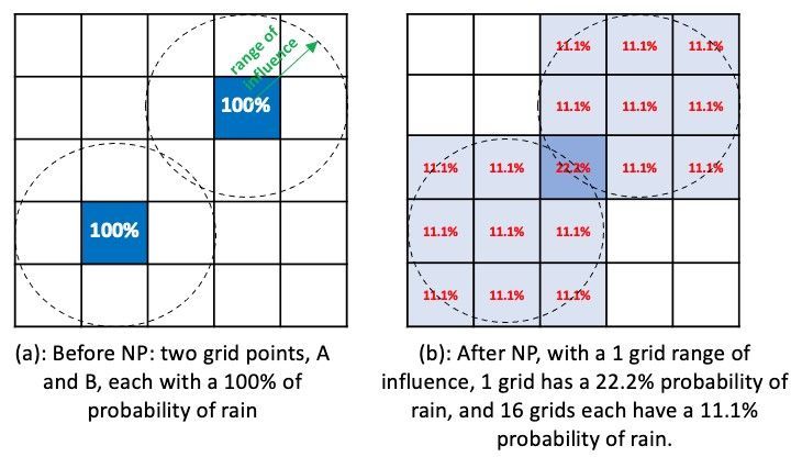
174 From Figure 1a, two grid points (“A” and “B”) each have a 100% probability of rain for a certain threshold.
175 Assuming that the influential grid range is 1, then after NP (Figure 1b), 16 grid points within the influential range
176 are considered each to have a probability of rain of 11.1%, while one grid will have a probability of 22.2%. The
177 NP method takes into account the spatial uncertainty of rainfall forecasts, increases the spread of the STEPS
178 produced ensemble, and helps smooth the probability output field (Ebert 2008).
179
180 At MetService, the NP method is implemented as below:
181 = {∑ 
 =0[ , (∑ =0 , , ]} (9)
 
182 where is the probability of rainfall at the threshold of mm, and , , is the ℎ STEPS ensemble member (at
183 the threshold of mm) from the base model . , is the weight for the base model .
184
185 Therefore , (∑ 
 =0 , , ) can be considered as the contributions of all the STEPS ensemble members from the

186 base model , where , is estimated using the Fractional Skill Score (e.g., Mittermaier, 2014) with one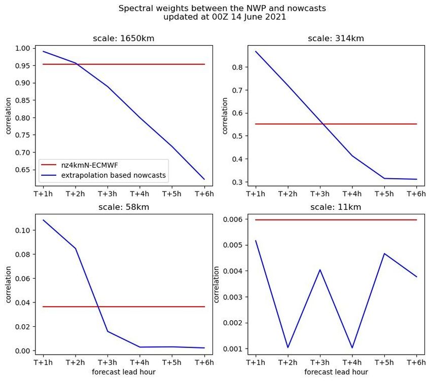

187 verification grid aggregated over the previous 12 hours. There may be other metrics that can be used for estimating
188 , , (e.g., using more than one verification grid for FSS), but the one presented here has been validated to work
189 in MetService’s operational environment. More studies may be carried out in the future to evaluate other metrics
190 for NP implementation at MetService.
191
192 The STEPS ensembles from different base models (with representing the total number of base models) are
193 combined and then the neighborhood processing, , is applied with the influential range of . At MetService, is
194 dynamically adjusted using the aggregated FSS for RainCast: the verification grid gradually increases from 1
195 ( = 1), and is recorded when FSS reaches an expected value . Note that at MetService is
196 threshold dependent (e.g., the expected FSS is 0.75 for the RainCast forecast at the threshold of 0.2 mm/h), and it
197 is determined by the requirement and specific needs of users of RainCast.

198 3. Case study
199 A heavy rainfall event from 00Z to 03Z on 14 June 2021 over the North Island of New Zealand is selected to
200 demonstrate the pros and cons of RainCast. This event occurred when a mesoscale low over the Tasman Sea (west
201 of North Island) slowly approached the upper North Island, while an associated front and rain band moved south
202 over Northland and Auckland (see Figure 3 for locations). Another front and rain band extended from the low
203 southwards towards Wellington. Figure 2 is a series of combined radar reflectivity images from the New Zealand
204 radar network obtained between 00Z and 03Z 14 June 2021, which shows that most of the North Island was
205 affected by a broad band of rainfall.
206
207 3.1 Experiment Setup
208 To evaluate the model skill between 00Z and 03Z on 14 June for different lead times (e.g., T+3 hours and T+24
209 hours), the forecasts from RainCast and the NWP models are compared. The initialization time of RainCast is
210 different from those of the NWP models, whose availability after initialization are dependent on the operational
211 environment at MetService.
212
213 The NWP models used in this comparison included the Global Forecast System (GFS) from NCEP, the Integrated
214 Forecast System (IFS) from ECMWF, and the Unified Model (UM) from the UKMO, and several LAM models
215 from MetService’s operational WRF running at a spatial resolution of 4.0 km. Table 1 gives the RainCast and the
216 corresponding NWP model analysis time (where the notation “nz4kmN-NCEP” represents the WRF model
217 initialized from the GFS global model from NCEP).
218
219 In Table 1, the latest NWP analysis time is determined by the arrival time of global model data. For example,
220 MetService receives most new NWP data every 12 hours from runs initialized at 00Z and 12Z. Therefore, for the
221 duration of this case study, the most recent NWP data available to forecasters would have been from the run
222 initialized at 12Z on 13 June, however they would not have seen this data until after 16Z on 13 June. In contrast
223 to the relatively slow delivery of NWP data, the latency of RainCast is approximately only 10-15 minutes, with a
224 moderate computational resource requirement.

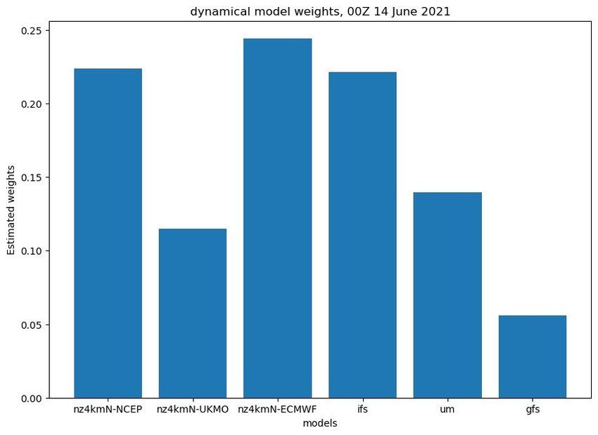
225
226 3.2 Runtime adjusted parameters
227 In this paper RainCast is “trained” by all the NWP models noted in Table 1. As described in Section 2.2, first the
228 evaluation is carried out for all candidate models so the best possible initial condition(s) for RainCast can be
229 utilized. For example, Figure 4 shows the model weights (at the threshold of 0.2 mm/h) estimated from the
230 objective model evaluation (noted as , in Section 2.2) between 12Z on 13 June and 00Z on 14 June. According
231 to this figure, the nz4kmN-ECMWF model (with an estimated weight of 0.24) performed better than the others at
232 the evaluation hour, and in RainCast it is assumed that this model would continue to perform well during the entire
233 forecast period. In this case, the lowest contribution for RainCast comes from the GFS model (with a weight of
234 0.05).
235
236 The “training” is also performed over the spectral space, as described in the STEPS algorithm (Section 2.1), to
237 merge the extrapolation-based nowcasts with NWP forecasts. Figure 5 shows the scale-dependent skills of
238 nz4kmN-ECMWF against the extrapolation-based nowcasts. The skill of both the nowcast and NWP degrades as
239 the spatial scale decreases (e.g., at a scale of 1650km the NWP has a correlation of 0.95, which decreases to 0.006
240 when the scale decreases to 11km).
241
242 The relative skills between the nowcast and NWP are also dependent on the spatial scale. For example, at the 1650
243 km scale, the extrapolation-based nowcast had better skill relative to the NWP out to T+2h, then after T+2h its
244 skill declined relative to NWP. Likewise, at the 314 km scale, the extrapolated nowcast had better skill in
245 comparison to the NWP out to T+3h, then afterwards its skill declined relative to the NWP. At a small scale (e.g.,
246 11 km), there is little skill from the extrapolation-based nowcast, and it is always lower than the NWP forecast.
247
248 Operationally, the above training process is carried out with the hourly updated cycle of RainCast. Such a frequent
249 update means that the latest NWP data can be utilized in the parameters’ estimation. However, the skill of
250 RainCast could be compromised because the training is performed over the entire domain, and it may not handle
251 well an event in a small area of interest (e.g., an area of most meteorological significance). Moreover, the weights
252 are estimated over the last 12 hours before RainCast’s analysis time, which does not necessarily mean these
253 weights will continue to produce the best skills for subsequent forecast hours.
254
255 3.3 Subjective Forecast evaluations
256 3.3.1 Forecast of rainfall probability vs QPE
257 Considering the contributions from the extrapolation-based nowcast, RainCast is expected to bring obvious
258 additional value to rainfall prediction within the first 1-2 hours. Additionally, with RainCast multiple NWP models
259 are evaluated and blended with the nowcast so improvements over a longer lead time can also be anticipated. In
260 this section, the predictions for 3-hour rainfall accumulation at the lead time of T+3h and T+24h are presented
261 and evaluated.
262

263 Figure 6 and Figure 7 compare the RainCast produced probability with the QPE product for the 3-hour rainfall
264 accumulation between 00Z and 03Z on 14 June with lead times of 3 hours and 24 hours respectively. The
265 thresholds applied for comparison are 2.0mm, 7.5mm and 15.0mm. Note that although QPE is considered as the
266 ground truth in this paper, it may come with various types of errors (Germann et al., 2006; Giangrande et al.,
267 2008; Zhang et al., 2011; Zhang et al., 2016) which are not discussed in this paper.
268
269 From Figure 6, the forecast probability of rain at a low threshold (e.g., 2.0mm) gives a good match to the QPE.
270 For example, high probabilities (>80%) of rainfall were predicted in a large area comprising Auckland,
271 Coromandel Peninsula, northern Waikato and western Bay of Plenty (see Figure 3 for locations. Coromandel
272 Peninsula is between Auckland and Bay of Plenty). High probabilities (between 50% and 90%) were given in
273 Wellington, while relatively lower probabilities (between 30% and 50%) were shown along the coast of the
274 Manawatu-Wanganui region. The skill of RainCast decreases with an increased threshold. For example, the area
275 with rainfall over 15.0mm was overestimated (although with relatively low probabilities), especially in the
276 Wellington region.
277
278 The skill of RainCast decreases with increasing lead hours. For example, Figure 7 gives the forecast rainfall
279 probability at the lead time of 24 hours. Compared to Figure 6, RainCast for the 2.0 mm threshold clearly over-
280 predicted in areas. For example, in the area including Taihape (central North Island) and inland Manawatu,
281 RainCast had a probability of greater than 30% of rain during the period of interest, whereas QPE showed it to be
282 dry. Moreover, little skill was shown when the threshold was increased to 7.5 mm.
283
284 The above study suggests that for this event, RainCast was generally good at distinguishing between wet and dry
285 areas although there were some overestimates (e.g., where the QPE showed it was dry, RainCast indicated a
286 probability of light or moderate precipitation). However, RainCast struggled to produce satisfactory results for
287 moderate-heavy rainfall intensities (e.g., 15 mm for a 3-hour period), especially when the lead time was longer
288 than 3 hours.
289
290 3.3.2 RainCast derived deterministic forecast vs other NWPs
291 To compare RainCast’s probabilistic forecasts with the deterministic rain forecasts from other models (i.e., IFS,
292 GFS, UM and WRF) used at MetService, three RainCast percentage probability levels were chosen to function as
293 pseudo “deterministic” rain forecasts. The percentage thresholds extracted from RainCast for this purpose were
294 25%, 50% and 75%.
295
296 Figure 8 shows the 3-hour rainfall accumulation forecasts from RainCast, IFS, GFS, UM, nz4kmN-NCEP,
297 nz4kmN-ECMWF and nz4kmN-UKMO, and they are compared to the QPE accumulation between 00Z and 03Z
298 on 14 June 2021 (model analysis time as in Table 1).
299
300 With reference to Figure 8, the IFS, RainCast (>25%) and RainCast(>50%) provided reasonable matches to the
301 QPE, especially in Northland, Auckland and Waikato. All three versions of RainCast, as well as the IFS and
302 UM models, compared reasonably well with the QPE for predicting rain in southern areas of Waikato, whereas

303 the nz4kmN-NCEP and nz4kmN-UKMO did not. However, there was a tendency in nearly all the models to
304 forecast much more rain than shown by the QPE over eastern Bay of Plenty and northern Taranaki, while all
305 three RainCast versions noticeably had much more rain in Wellington compared to the QPE. Overall, IFS and
306 the two RainCast versions (>25% and 50%) appear to have outperformed the others in this subjective
307 comparison.
308
309 As already noted, in contrast to the QPE there was significant rainfall predicted by many of the models (including
310 RainCast) over eastern Bay of Plenty. A reason for this is that radar coverage of the area is compromised. The
311 distance to the radar station in the western Bay of Plenty means that the low-tropospheric rain cannot be observed
312 well with the QPE underestimating the rain as a result, while the radar station in Hawkes Bay will suffer from
313 beam blocking in the lowest elevations to the north/northwest. Installing and using more rain gauges in the radar
314 rainfall calibration process could provide us with a better QPE map, which is a possibility for future improvement.
315
316 Similar to Figure 8, when the lead time was 24 hours (Figure 9), IFS and the two RainCast forecasts (>25% and
317 50%) seemed generally to outperform the other models. However, these three approaches under-forecasted rain
318 along the coast of Waikato, although the RainCast (>25%) was slightly better than the other two. There are
319 massive overestimates in the Bay of Plenty compared to the QPE. Some spurious showers were presented in the
320 Manawatu-Wanganui region from IFS and RainCast (>25%), which were successfully eliminated when the
321 probability threshold increased to 50% in RainCast. In contrast, the rest of the models (e.g., GFS, UM and all
322 WRFs) did not give good predictions for a lead time of 24 hours.
323
324 The above indicates that RainCast was overall able to provide improved forecasts compared to most individual
325 NWP approaches, especially over a short range (e.g., < 3 hours). For this event IFS gave comparable results to
326 RainCast. However, to evaluate the ability of RainCast over a longer period, a more quantitative and less
327 subjective evaluation approach must be adopted, which is described in Section 4.

328 4. Objective verification
329 Section 3 provides a subjective evaluation of the event that occurred between 00Z and 03Z on 14 June. However,
330 such an evaluation is not carried out quantitatively, and it is prone to individual biases of interpretation (e.g.,
331 Stanski et al., 1989). To objectively validate the accuracy of forecasts, it is more useful to calculate the FSS over
332 a longer period, as presented here for the period 00Z 1 June 2021 to 30 June 2021. During this period numerous
333 rain-producing systems of varied intensities affected the country (the case presented in Section 3 is one of the
334 events that occurred during this period).
335
336 One of the challenges of applying the FSS is the different spatial resolutions of the models. For example, the
337 effective QPE resolution for New Zealand is 5.0 km, while RainCast, IFS, GFS, UM and WRF (including
338 nz4kmN-NCEP, nz4kmN-UKMO and nz4kmN-ECMWF) have resolutions of approximately 5.0km, 9.0km,
339 22.0km, 25.0km and 4.0km, respectively. To calculate the FSS, all the models are re-projected to the QPE grid,
340 meaning that the base resolution for the verification is 5.0 km which may be different to the effective resolution
341 of a particular model. Figure 10 shows the FSS with different thresholds (0.5mm, 7.5mm and 15.0 mm) on

342 verification grids of 1 (5.0 km) and 5 (25.0 km), respectively. The scores are calculated by validating 3-hour rain
343 accumulations at 3 hourly intervals throughout the 1 month duration.
344
345 At a threshold of 0.5mm RainCast (>25%) outperformed all the other models over the entire 24 hours, (Figure
346 10A and 10B). IFS produced the highest skill score among the global NWP models. UM scored the lowest over
347 the aggregation period with 1 verification grid, however its performance improved when the number of
348 verification grids increased. For example UM performed better than RainCast (>75%) when the grid increased to
349 5, (Figure 10B). Verification also indicates that RainCast (>75%) gave a low number of both “hits” and “false
350 alarms”, and on average its skill is lower than most other forecast approaches at such a small verification threshold.
351
352 When the threshold increased to 7.5 mm (Figure 10C and 10D), the skill of RainCast (> 25%) dropped below IFS
353 and nz4kmN-ECMWF, especially after 3-6 hours. RainCast (>75%) provided the best forecasts from the FSS
354 point of view, followed by RainCast (>50%). On average, IFS still ranked third among all forecast approaches.
355 Moreover, the skill of UM increased with increased verification scale. For example, UM performed slightly better
356 than the nz4kmN-UKMO when the number of verification grids increased to 5, especially after T+12 hours.
357
358 When the verification threshold is increased, forecast skill significantly reduces (Figure 10E and 10F). For
359 example, the average skill for all forecast approaches dropped from 0.65 (threshold of 0.5mm using 1 verification
360 grid, Figure 10A) to 0.13 (threshold of 15.0mm using 1 verification grid, Figure 9E). Similar to the verification
361 with a threshold of 7.5mm, RainCast (>75%) on average still performed the best from the FSS point of view,
362 especially for the first 3-6 hours. In contrast to the verifications with lower thresholds (Figure 10A, 10B, 10C and
363 10D), IFS outperformed RainCast (>50%). On the other hand, RainCast (>25%) did not provide satisfactory
364 results due to its overestimates at such a threshold.
365
366 It is worthwhile to note that the objective verification (FSS) used in this paper does not necessarily reflect the
367 “goodness” or “usefulness” of the forecast. From an operational forecast point of view, “consistency”, “quality”
368 and “value” are the three essential metrics which determine the usefulness of a forecast (e.g., Murphy, 1993,
369 1995), while objective verification mainly provides a reference for the forecast quality.
370
371 RainCast frequently uses the latest available observations, and this inevitably means that the user will have to
372 expect more inconsistencies from updated forecasts cycle by cycle. Moreover, since RainCast is a statistical
373 system and is not constrained by physical laws which the NWP-based systems are, this could lead to discrepancies
374 between the output from RainCast and the forecaster’s best judgement about the situation, which usually takes
375 many meteorological factors into account.
376
377 Additionally, the above objective verification is carried out and averaged over the entire New Zealand domain,
378 which may not optimally reflect the situation in an area or areas where there are more meteorological values of
379 significance (e.g., a thunderstorm in a city is likely to have greater impact than one which occurs in an uninhabited
380 area). Therefore, even though the FSS has value in quantifying how RainCast performs, it will take longer in an
381 operational environment to fully realise the benefits that can be gained by decision makers using its forecasts.

382 5. Discussion:
383 The skills of RainCast were demonstrated in both Section 3 and Section 4. In this section, the system limitations
384 and potential improvements are discussed.
385
386 RainCast uses radar data to produce extrapolated nowcasts, and to evaluate the initial conditions of the different
387 NWP models for the current hour (or latest RainCast analysis time). The QPE data, which is used to verify the
388 results from RainCast and other forecast models, are also largely dependent on radar data. Therefore, the quality
389 of radar data plays an essential role in the running of RainCast, and consequently the skill of the system is
390 dependent on it, especially for the first few hours.
391
392 The topography of New Zealand is complex, especially in the South Island. For example, the Southern Alps run
393 almost along the whole length of the island, which are approximately 800km long and more than 60 km wide, and
394 therefore forms an effective barrier between western and eastern areas of the island. Consequently, New Zealand’s
395 complex orography often obstructs low-level radar beams, degrading the performance of radar-based nowcasting
396 (e.g., Foresti and Seed, 2015).
397
398 Another major uncertainty from the use of radar data is the Z-R relationship. At MetService, a customized Z-R
399 relationship is used to convert radar observed reflectivity to rainfall amounts. This Z-R relationship is updated
400 hourly by regressing the dBZ to gauge-observed rainfall (not presented in this paper). It is demonstrated in an
401 operational environment that this dynamically adjusted Z-R relationship matches the rain gauge records more
402 accurately for New Zealand than the Marshall-Palmer distribution = 200 1.6 (Marshall and Palmer, 1948), but
403 still underestimates many significant events, especially when the reflectivity is greater than 20-25 dBZ.
404
405 Since a lot of rain gauge data cannot be retrieved in a timely manner to correct it for use in RainCast, there will
406 consequently be underestimates in the extrapolation-based nowcasts, and thus a downgrade in the performance of
407 RainCast, especially for the first 1 to 3 hours. This issue will also affect RainCast’s initial conditions and forecast
408 evaluation, since the QPE, which is largely derived from radar data, is here considered as the “ground truth”. It is
409 recommended that an improved radar quality control system is needed to further improve the skill of RainCast.
410
411 As described in Section 2, there are multiple NWP models used in RainCast and they are blended with an
412 extrapolation-based nowcast. The contribution from an individual NWP model is dependent on its skill over a
413 predefined aggregation period (usually it is between T+0h and T+12h where T+0h is the RainCast analysis time).
414 However, such a skill does not necessarily reflect the model’s performance for subsequent hours, especially if
415 there are changes to how a weather situation evolves. Moreover, this skill is estimated over the entire RainCast
416 domain, and the domain average skill may not represent a particular area of interest (e.g., airports, urban centres
417 with dense populations and areas exposed to the highest risk of flooding). One of the potential improvements that
418 could be made in the future is to run RainCast over a smaller domain specifically for the area with the most
419 meteorological value.

420 6. Summary:
421 The hourly updated RainCast system at MetService has been described. The algorithm for this system is adapted
422 from STEPS with a neighborhood processing method applied. This system is in the process of being implemented
423 operationally at MetService. Evaluation suggests that, compared to the NWP alone approach, RainCast could
424 improve precipitation forecasts in New Zealand out to 24 hours, particularly for light to moderate rainfall events,
425 with the greatest improvements in the first 1-3 hours.
426

427 Acknowledgement
428 The authors thank several MetService operational forecasters for providing valuable feedback during the RainCast
429 forecast demonstration project. The authors also thank Dr. Alan Seed (Bureau of Meteorology, Australia) for
430 providing suggestions and guidance on the implementation of the STEPS algorithm in New Zealand. The idea of
431 blending multiple models was inspired by Dr. Xiang-yu Huang (Meteorological Service Singapore) and Dr.
432 Juanzhen Sun (National Center for Atmospheric Research, Boulder, USA). Global model data were obtained from
433 NCEP, UK Met Office and ECMWF. The WRF model was developed and provided by NCAR. Some of the rain
434 gauge observations used in this paper were provided by the local regional councils in New Zealand.
435

436 References
437
438 Barker, D. M., W. Huang, Y.R. Guo, A. J. Bourgeois and Q. N. Xiao (2004). A three-dimensional variational
439 data assimilation system for MM5: Implementation and initial results. Mon. Wea. Rev., 132, 897–914.

440 Benjamin, S. G., et al. (2004a). An hourly assimilation/forecast cycle: The RUC. Mon. Wea. Rev.,132, 495–518.

441 Benjamin, S. G., et al. (2016). A North American hourly assimilation and model forecast cycle: The Rapid Refresh.
442 Mon. Wea. Rev.,144, 1669–1694.

443 Bowler, N. E., Pierce, C. E., and Seed, A. W. (2006). STEPS: A probabilistic precipitation forecasting scheme
444 which merges an extrapolation nowcast with downscaled NWP, Q. J. R. Meteorol. Soc., 132, 2127–2155.

445 Browning, K. A. (1980). Local weather forecasting. Proc. Roy. Soc. London, A371, 179–211.

446 Clark, A. J., J. Gao, P. T. Marsh, T. Smith, J. S. Kain, J. Correia, M. Xue, and F. Kong (2013). Tornado
447 pathlength forecasts from 2010 to 2011 using ensemble updraft helicity. Wea. Forecasting, 28, 387–407.

448 Dixon, M. and G. Wiener (1993). TITAN: Thunderstorm Identification, Tracking, Analysis, and Nowcasting—A
449 radar-based methodology. J. Atmos. Oceanic Technol., 10, 785–797.

450 Ebert, E. (2008). Fuzzy verification of high-resolution gridded forecasts: A review and proposed
451 framework. Meteor. Appl., 15, 51–64.

452 Foresti, L.; Seed, A. (2015). On the spatial distribution of rainfall nowcasting errors due to orographic forcing.
453 Meteorol. Appl. 2015, 22, 60–74.

454 Gagne, D. J., A. McGovern, J. Brotzge, M. Coniglio, J. Correia Jr., and M. Xue (2015). Day-ahead hail
455 prediction integrating machine learning with storm-scale numerical weather models. 27th Conf. on Innovative
456 Applications of Artificial Intelligence, Austin, TX, Association for the Advancement of Artificial
457 Intelligence, 3954–3960.

458 Germann, U., and I. Zawadzki (2002). Scale-dependence of the predictability of precipitation from continental
459 radar images. Part I: Description of the methodology. Mon. Wea. Rev., 130, 2859–2873.

460 Germann, U., G. Galli, M. Boscacci, and M. Bolliger (2006). Radar precipitation measurement in a mountainous
461 region. Quart. J. Roy. Meteor. Soc., 132, 1669–1692.

462 Giangrande, S. E., and A. V. Ryzhkov (2008). Estimation of rainfall based on the results of polarimetric echo
463 classification. J. Appl. Meteor. Climatol., 47, 2445–2462.

464 Haiden, T., Kann, A., Wittmann, C., Pistotnik, G., Bica, B., and Gruber, C. (2010). The Integrated Nowcasting
465 through Com- prehensive Analysis (INCA) System and Its Validation over the Eastern Alpine Region, Wea.
466 Forecasting, 26, 166–183.

467 Jirak, I. L., C. J. Melick, and S. J. Weiss (2014). Combining probabilistic ensemble information from the
468 environment with simulated storm attributes to generate calibrated probabilities of severe weather hazards. 27th
469 Conf. on Severe Local Storms, Madison, WI, Amer. Meteor. Soc., 2.5, https://ams.confex.com/ams/
470 27SLS/webprogram/Paper254649.html.

471 Lovejoy, S. D. Schertzer (2006). Multifractals, cloud radiances and rain, J. Hydrol. 322, 59-88.

472 Lynn, B. H., G. Kelman, and G. Ellrod (2015). An evaluation of the efficacy of using observed lightning to
473 improve convective lightning forecasts. Wea. Forecasting, 30, 405–423.

474 Mittermaier, M. (2014). A strategy for verifying near-convection-resolving forecasts at observing sites. Wea.
475 Forecasting, 29, 185–204.

476 Marshall, J. S. and Palmer, W. M. (1948): The distribution of raindrops with size, J. Meteor., 5, 165–166.

477 Milan, M., Macpherson, B., Tubbs, R. (2020). Hourly 4D-Var in the Met Office UKV operational forecast
478 model. Q. J. R. Meteorol. Soc. 146, 1281– 1301.

479 Murphy, A.H. (1993). What is a good forecast? An essay on the nature of goodness in weather forecasting. Wea.
480 Forecasting, 8, 281-293.

481 Murphy, A.H. (1995). The coefficients of correlation and determination as measures of performance in forecast
482 verification. Wea. Forecasting, 10, 681-688.

483 Huang, X.-Y., et al. (2009). Four-dimensional variational data assimilation for WRF: Formulation and
484 preliminary results. Mon. Wea. Rev., 137, 299–314.

485 Roberts, N. M., and H. W. Lean (2008). Scale-selective verification of rainfall accumulations from high-
486 resolution forecasts of convective events. Mon. Wea. Rev., 136, 78–97.

487 Schwartz, C.S., et al. (2010). Toward Improved Convection-Allowing Ensembles: Model Physics Sensitivities
488 and Optimizing Probabilistic Guidance with Small Ensemble Membership. Wea. Forecast, 25, 263–280.

489 Schwartz, C.S. and Ryan A.S. (2017). Generating Probabilistic Forecasts from Convection-Allowing Ensembles
490 Using Neighbourhood Approaches: A Review and Recommendations. Mon. Wea. Rev. 2017, 145(9), 3397–341.

491 Seed, A. W. (2003). A Dynamic and Spatial Scaling Approach to Advection Forecasting, J. Appl. Meteor., 42,
492 381–388.

493 Seed, A.E., C. E. Pierce, and K. Norman. (2013). Formulation and evaluation of a scale decomposition-based
494 stochastic precipitation nowcast scheme. Water Resources Research, 49(10): 6624–6641.

495 Snyder, C., and F. Zhang (2003). Assimilation of simulated Doppler radar observations with an ensemble Kalman
496 filter. Mon. Wea. Rev., 131, 1663–1677.

497 Skamarock, W. C., et al. (2008). A description of the Advanced Research WRF version 3. NCAR Tech. Note.
498 NCAR/TN-4751STR, 113 pp.

499 Sobash, R. A., J. S. Kain, D. R. Bright, A. R. Dean, M. C. Coniglio, and S. J. Weiss. (2011). Probabilistic forecast
500 guidance for severe thunderstorms based on the identification of extreme phenomena in convection-allowing
501 model forecasts. Wea. Forecasting, 26, 714–728.

502 Sobash, R. A., C. S. Schwartz, G. S. Romine, K. R. Fossell, and M. L. Weisman (2016). Severe weather
503 prediction using storm surrogates from an ensemble forecasting system. Wea. Forecasting, 31, 255–271.

504 Stanski, H.R., L.J. Wilson, and W.R. Burrows (1989). Survey of common verification methods in meteorology.
505 World Weather Watch Tech. Rept. No.8, WMO/TD No.358, WMO, Geneva, 114 pp.

506 Sun, J., M. Chen and Y. Wang (2010). A frequent-updating analysis system based on radar, surface, and
507 mesoscale model data for the Beijing 2008 forecast demonstration project. Wea. Forecasting, 25, 1715–1735.

508 Sun, J., S. B. Trier, Q. Xiao, M. L. Weisman, H. Wang, Z. Ying, M. Xu, and Y. Zhang (2012). Sensitivity of 0–
509 12-h warm-season precipitation forecasts over the central United States to model initialization. Wea.
510 Forecasting, 27, 832–855.

511 Theis, S. E., A. Hense, and U. Damrath (2005). Probabilistic precipitation forecasts from a deterministic model:
512 A pragmatic approach. Meteor. Appl., 12, 257–268.

513 Wang, X. G., Parrish, D., Kleist, D., & Whitaker, J. (2013). GSI 3DVarbased ensemble-variational hybrid data
514 assimilation for NCEP global forecast system: Single-resolution experiments. Monthly Weather Review, 141,
515 4098– 4117.

516 Wilson, J. W., and R. D. Roberts (2006). Summary of convective storm initiation and evolution during IHOP:
517 Observational and modelling perspective. Mon. Wea. Rev., 134, 23–47.

518 Xiao, Q., Y.-H. Kuo, J. Sun, W.-C. Lee, D. M. Barker, and E. Lim. (2007). An approach of radar reflectivity data
519 assimilation and its assessment with the inland QPF of Typhoon Rusa (2002) at landfall. J. Appl. Meteor.
520 Climatol., 46, 14–22.

521 Zhang, J., et al. (2011). National mosaic and multi-sensor QPE (NMQ) system: Description, results, and future
522 plans. Bull. Amer. Meteor. Soc., 92, 1321–1338.

523 Zhang, J., et al. (2016). Multi-Radar Multi-Sensor (MRMS) quantitative precipitation estimation: Initial operating
524 capabilities. Bull. Amer. Meteor. Soc., 97, 621–638.

525 Zhang, S., G. Austin, and L. Sutherland. (2014). The implementation of reverse Kessler warm rain scheme for
526 radar reflectivity assimilation using a nudging approach in New Zealand. Asia-Pacific J. Atmos. Sci., 50(3), 283-
527 296.

Figures

Figure 1

An illustrated description of neighborhood processing (probabilities are calculated to three signi cant
 gures)

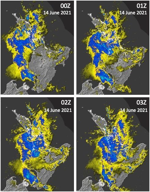
Figure 2

A series of radar re ectivity images between 00Z and 03Z 14 June 2021.

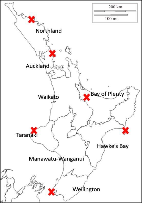
Figure 3

Regions of the North Island of New Zealand (courtesy to LGNZ: https://www.lgnz.co.nz), and locations of
the rain radars (red crosses).

Figure 4

Dynamically adjusted weights at 00Z 14 June 2021 for all available NWP models.

Figure 5

Correlations between the extrapolation-based nowcasts (blue) and NWP (red) for different spatial scales
(updated at 00Z 14 June 2021).

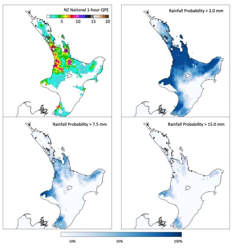
Figure 6

RainCast rainfall probability (3-hour accumulation) between 00Z and 03Z, 14 June 2021, and the
corresponding QPE (top-left). The RainCast analysis time is 00Z 14 June 2021.

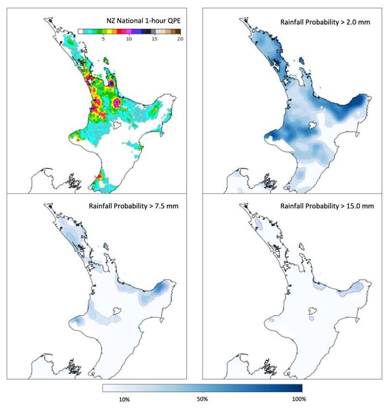
Figure 7

As Figure 6, but the RainCast analysis time is 03Z 13 June 2021.

Figure 8

QPE (far left) and 3-hour rainfall accumulations valid between 00Z and 03Z 14 June 2021 for nine
different forecast approaches. Analysis times for the models are as in Table 1.

Figure 9

As Figure 8, but with forecast lead time of 24 hours.

Figure 10

FSS aggregated between 00Z 1 June and 23Z 30 June 2021.