Examensarbete 15 hp Juni 2021 - Resonance frequency, Q-factor, coupling of a cylindrical cavity and the effect on graphite from an alternating ...
←
→
Page content transcription
If your browser does not render page correctly, please read the page content below
MAT-VET-F-21020
                    Examensarbete 15 hp
                             Juni 2021

Resonance frequency, Q-factor, coupling
 of a cylindrical cavity and the effect on
graphite from an alternating electric field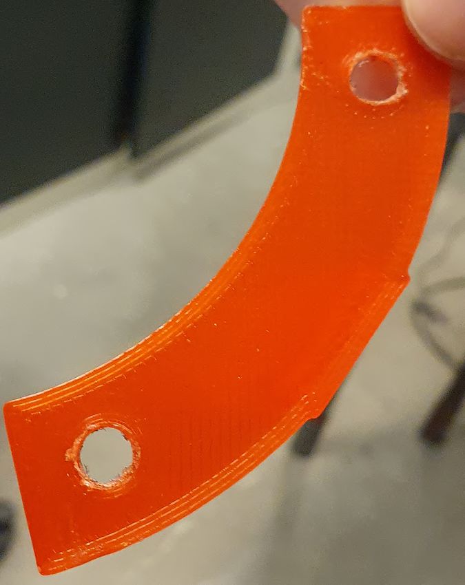
Abstract

                                  Jakob Gölén, Simon Persson

                                  The purpose of this project was to investigate a cylindrical cav-
                                  ity resonator and use microwaves to heat up a material in the
                                  cavity. This was done by measuring the Q-factor and the reso-
                                  nance frequency of the cavity, both with and without material
                                  inside. The chosen material was graphite, and more accurate
                                  measurements were done with that specific material. A pro-
                                  gram called QZero was used to export the Q-factor and the res-
                                  onance frequency from the measurement data received from a
                                  VNA and the program also gave error estimations. Then elec-
                                  tromagnetic simulations were done using Comsol. Both an
                                  empty cavity and a cavity where graphite has been inserted
                                  were simulated and the results were compared to the actual
Teknisk- naturvetenskaplig        measurements. To measure temperatures inside the cavity, a
fakultet UTH-enheten              pyrometer was to be used. The cavity resonator has small cir-
                                  cular holes through the side, and a frame was designed and
Besöksadress:                    produced using a 3D-printer in order to lock the pyrometer
Ångströmslaboratoriet           in place in front of one of the holes. A power supply was
Läderhyddsvägen 1               also installed to the pyrometer. In order to send microwaves
Hus 4, Plan 0                     into the cavity, a signal generator was used. It was connected
Postadress:                       to an amplifier and the amplification as well as the efficiency
Box 536                           was noted. The pyrometer could only measure temperatures
751 21 Uppsala                    above 490 ◦ C. This was not achieved, so a handheld electrical
                                  thermometer was used. The temperature of the graphite was
Telefon:                          measured and then compared to how hot the graphite would
018 - 371 30 03                   be without heat loss.
                                       For the empty cavity, a Q-factor of 3200 for the resonance
Telefax:
                                  frequency of around 2.4 GHz was measured, which matched
018 - 471 30 00
                                  the simulated measurements in Comsol. When graphite was
Hemsida:                          inserted to the cavity, the Q-factor lowered to 300 in the real
http://www.teknat.uu.se/student   experiment. A discrepancy was found between the actual mea-
                                  surements, and the Comsol simulations in which the graphite
                                  only lowered the Q-factor to 2570. The reason for this is be-
                                  lieved to be either with an error to how the material was chosen
                                  in Comsol, since there were many types of graphite to select
                                  with many settings to change. Another reason could be an
                                  error with the setup itself due to the sheer complexity of the
                                  program.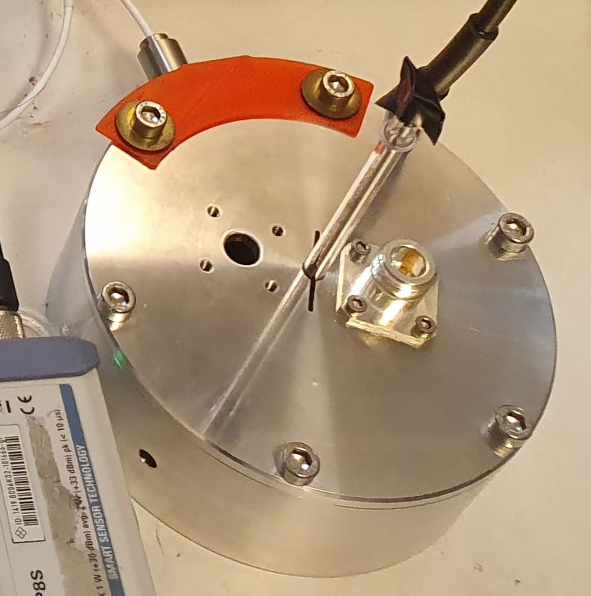
For the heating experiment, the amplifier was determined to
                                  have a low efficiency for power outputs under 5 W which re-
Teknisk- naturvetenskaplig        sulted a in risk of overheating the amplifier. For this reason
fakultet UTH-enheten              only low power could be used. For an output of 2 W, the
                                  graphite was heated to 100-150◦ C from 30 seconds of expo-
Besöksadress:                    sure to the microwaves. This was significantly lower than the
Ångströmslaboratoriet           theoretical value of 1700◦ C calculated from the energy pro-
Läderhyddsvägen 1               vided to the graphite, which leads to a theory that the temper-
Hus 4, Plan 0                     ature found an equilibrium at around 100-200◦ C or that the
Postadress:                       resonance frequency changes such that the graphite could no
Box 536                           longer absorb the energy.
751 21 Uppsala
Telefon:
018 - 371 30 03
Telefax:
018 - 471 30 00
Hemsida:
http://www.teknat.uu.se/student

                                  Handledare: Dragos Dancila
                                  Ämnesgranskare: Maria Strömme
                                  Examinator: Martin Sjödin
                                  ISSN; 1401-5757, MAT-VET-F-21020
                                  Tryckt av: Uppsala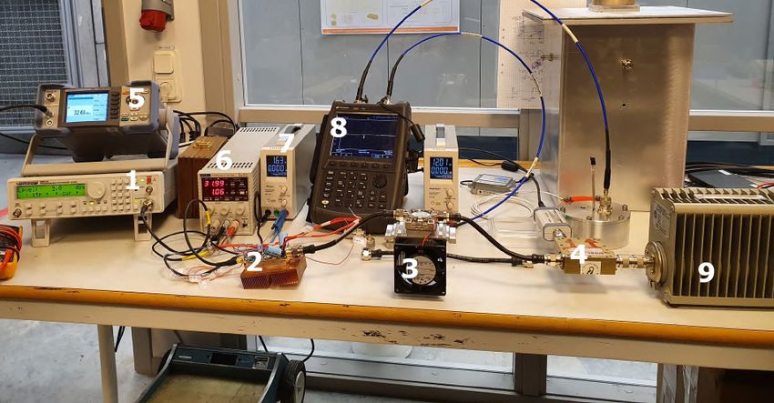
Kurs: Självständigt arbete i teknisk fysik                     Jakob Gölén, Simon Persson

Populärvetenskaplig sammanfattning
Syftet med detta projekt är att undersöka en cylindrisk kavitet samt att använda mikrovågor
för att värma upp ett material i kaviteten. Detta gjordes genom att mäta kavitetens Q-faktor
och resonansfrekvens med och utan material. Sedan valdes grafit ut som det materialet som
skulle testas och mer noggranna mätningar gjordes på just det materialet, och programmet
QZero användes för att få ut mer noggrann data samt gav en felmarginal på Q-faktorn.
Efter det gjordes simuleringar i programmet Comsol av kaviteten med och utan grafit och
jämfördes med de faktiska värdena. För att mäta temperatur av materialet i kaviteten desig-
nades en hållare som en pyrometer skulle fästas vid och riktas mot materialet i kaviteten.
Även en strömförsörjning till pyrometern installerades. För att skicka in mikrovågor i
kaviteten användes en signalgenerator som var kopplad till en förstärkare. Förstärknin-
gen mättes och förstärkarens effekt noterades. I slutändan nåddes inte de temperaturer
som krävdes för pyrometern, så en elektrisk termometer användes för att mäta tempera-
turen på grafiten och detta jämfördes sedan mot den energin som absorberades av grafiten,
då energin tillförd till grafiten och grafitens specifika värmekapacitet var känt. Prestan-
dan av experimentuppställningen undersöktes också. For den tomma kaviteten mättes en
Q-faktor på 3200 och resonansfrekvensen var 2.4 GHz. Detta stämde bra överens med
simuleringarna i Comsol. När grafit fördes in i kaviteten sänktes Q-faktorn till 300. En
avvikelse upptäcktes mellan de faktiska mätningarna och simuleringarna. I simuleringen
sänktes Q-faktorn bara till 2570, en andledning till detta tros vara antingen vara hur ma-
terialet valdes, då det fanns olika typer av grafit med olika inställningar att välja mellan i
Comsol. En annan felkälla kan vara något fel med uppställningen på grund af hur avancerat
Comsol var. I värmeexperimentet hade förstärkaren en låg verkningsgrad vilket ledde till
överhettning om för stor effekt användes. Experimentet begränsades därför till att använda
upp till två watt. Vid exponerig under 30 sekunder värmdes grafiten upp till 100-150◦ C,
vilket var avsevärt lägre än den teoretiska uppvärmingen till 1700◦ beräknad från ener-
gin tillförd till grafiten. Antagandet är att temperaturen hamnade i ett jämnviktsläge kring
100-200◦ C eller att resonansfrekvensen ändrades vilket ledde till en minskning av energi
tillförd till grafiten.
Kurs: Självständigt arbete i teknisk fysik                                             Jakob Gölén, Simon Persson

1   Introduction                                                                                                                             1
    1.1 Goal . . . . . . . . . . . . . . . . . . . . . . . . . . . . . . . . . . . . .                                                       1

2   Theory                                                                                                                                   2
    2.1 Q-factor, scattering . . . . . . . . . .                 .   .   .   .   .   .   .   .   .   .   .   .   .   .   .   .   .   .   .   2
    2.2 Coupling coefficient . . . . . . . . . .                 .   .   .   .   .   .   .   .   .   .   .   .   .   .   .   .   .   .   .   3
    2.3 The cavity and resonance frequencies                     .   .   .   .   .   .   .   .   .   .   .   .   .   .   .   .   .   .   .   3
    2.4 Smith diagram . . . . . . . . . . . . .                  .   .   .   .   .   .   .   .   .   .   .   .   .   .   .   .   .   .   .   4
    2.5 Vector network analyser . . . . . . .                    .   .   .   .   .   .   .   .   .   .   .   .   .   .   .   .   .   .   .   5
    2.6 Signal generator . . . . . . . . . . . .                 .   .   .   .   .   .   .   .   .   .   .   .   .   .   .   .   .   .   .   5
         2.6.1 dBm . . . . . . . . . . . . . .                   .   .   .   .   .   .   .   .   .   .   .   .   .   .   .   .   .   .   .   5
    2.7 Amplifier . . . . . . . . . . . . . . .                  .   .   .   .   .   .   .   .   .   .   .   .   .   .   .   .   .   .   .   6
    2.8 Directional coupler . . . . . . . . . .                  .   .   .   .   .   .   .   .   .   .   .   .   .   .   .   .   .   .   .   6
    2.9 Circulator . . . . . . . . . . . . . . .                 .   .   .   .   .   .   .   .   .   .   .   .   .   .   .   .   .   .   .   7
    2.10 Electric heating . . . . . . . . . . . .                .   .   .   .   .   .   .   .   .   .   .   .   .   .   .   .   .   .   .   7
    2.11 Comsol . . . . . . . . . . . . . . . .                  .   .   .   .   .   .   .   .   .   .   .   .   .   .   .   .   .   .   .   7
    2.12 QZero . . . . . . . . . . . . . . . . .                 .   .   .   .   .   .   .   .   .   .   .   .   .   .   .   .   .   .   .   8
         2.12.1 Purpose . . . . . . . . . . . .                  .   .   .   .   .   .   .   .   .   .   .   .   .   .   .   .   .   .   .   8
         2.12.2 Inner workings . . . . . . . .                   .   .   .   .   .   .   .   .   .   .   .   .   .   .   .   .   .   .   .   8
         2.12.3 Error estimation . . . . . . .                   .   .   .   .   .   .   .   .   .   .   .   .   .   .   .   .   .   .   .   9

3   Method                                                                                                                                   11
    3.1 Material . . . . . . . . . .     .   .   .   .   .   .   .   .   .   .   .   .   .   .   .   .   .   .   .   .   .   .   .   .   .   11
    3.2 Measurements of material .       .   .   .   .   .   .   .   .   .   .   .   .   .   .   .   .   .   .   .   .   .   .   .   .   .   13
    3.3 Accurate measurements . .        .   .   .   .   .   .   .   .   .   .   .   .   .   .   .   .   .   .   .   .   .   .   .   .   .   13
    3.4 The Pyrometer . . . . . .        .   .   .   .   .   .   .   .   .   .   .   .   .   .   .   .   .   .   .   .   .   .   .   .   .   14
    3.5 The heating experiment . .       .   .   .   .   .   .   .   .   .   .   .   .   .   .   .   .   .   .   .   .   .   .   .   .   .   15
    3.6 Comsol . . . . . . . . . .       .   .   .   .   .   .   .   .   .   .   .   .   .   .   .   .   .   .   .   .   .   .   .   .   .   17

4   Results and Discussion                                                                                                                   18
    4.1 Results . . . . . . . . . . . . . . . . . . . . . . . . . . . . .                                        .   .   .   .   .   .   .   18
         4.1.1 Material study . . . . . . . . . . . . . . . . . . . .                                            .   .   .   .   .   .   .   18
         4.1.2 Measurements with the VNA and in Comsol . . . .                                                   .   .   .   .   .   .   .   18
         4.1.3 Amplification and efficiency of amplifier . . . . . .                                             .   .   .   .   .   .   .   20
         4.1.4 Heating of graphite . . . . . . . . . . . . . . . . . .                                           .   .   .   .   .   .   .   22
    4.2 Discussion . . . . . . . . . . . . . . . . . . . . . . . . . . .                                         .   .   .   .   .   .   .   22
         4.2.1 Material study . . . . . . . . . . . . . . . . . . . .                                            .   .   .   .   .   .   .   22
         4.2.2 VNA and Comsol measurements obtained by QZero                                                     .   .   .   .   .   .   .   22
         4.2.3 Heating experiment . . . . . . . . . . . . . . . . . .                                            .   .   .   .   .   .   .   22

                                                     III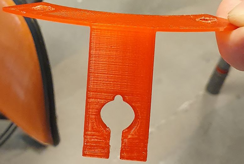
Kurs: Självständigt arbete i teknisk fysik                 Jakob Gölén, Simon Persson

5   Conclusion                                                                          23
    5.1 Whats next? . . . . . . . . . . . . . . . . . . . . . . . . . . . . . . . . .   23

6   References                                                                          25

                                               IV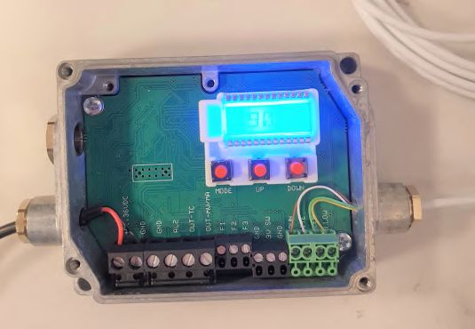
Kurs: Självständigt arbete i teknisk fysik                   Jakob Gölén, Simon Persson

1      Introduction
Since the 1940s, microwave technology for the purpose of heating have developed rapidly
and is today commonplace. Microwave heating works by sending energy directly into the
material, which then absorbs it. This creates a disturbance in the electron cloud surround-
ing the molecule of the material targeted by the microwaves. A dipole moment is induced
and the friction from the movement creates heat, which in turn heats the material.
    Microwave heating has many benefits over other, traditional heating processes. It is
very energy efficient, since the heating occurs within the material itself, minimizing wasted
energy that heats the materials surroundings. Microwave components can also be built to
a smaller scale than other heating processes and greater control over the heating process
is possible.(1) The most interesting case for microwave heating today is the possibility
of 3D-printing with dielectric materials. If made possible a lot of energy could be saved
and a more even melting procedure could be done with higher temperatures. This would
mainly work for metals but could be done on plastic by blending the plastic with dielectric
materials. An example of metal sintering can be found in the 47th European Microwave
Conference under (Samuel Hefford 1, Nyle Parker 2, Jonathan Lees 3, and Adrian Porch
4, ”Monitoring Changes in Microwave Absorption of Ti64 Powder During Microwave
Sintering”).

1.1     Goal
The goal with this project was to investigate a microwave cavity and use it to heat mate-
rials, which in this project was graphite powder. This main goal was then divided into a
number of smaller subgoals:

      • How to measure the Q-factor and resonance frequency of the cavity, two important
        properties. This included learning about the measurement equipment (VNA) and
        what the data consists of (Scattering parameters).

      • Doing the measurements in goal 1.

      • Simulate the cavity in Comsol and compare the data to the actual data obtained on
        location.

      • Setting up and doing the actual experiment. This included finding a way to measure
        the temperature in the cavity (pyrometer and how to fit the pyrometer to the cavity),
        as well as measuring the temperature of the graphite and compare it to what would
        reasonably happen.

                                               1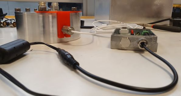
Kurs: Självständigt arbete i teknisk fysik Jakob Gölén, Simon Persson
2 Theory
2.1 Q-factor, scattering
To understand the experiment, it is crucial to at least have heard about a couple of im-
portant terms. One of which is the quality factor. The Q-factor can be described as how
much power in in the form of the input signal is stored inside the system compared to the
dissipated energy per wavelength as shown in equation 1. In simpler terms, a low Q-factor
means that a lot of the energy is absorbed inside the system while a high Q-factor points
towards a low absorption. When changing the heat of a system it may be interesting to
analyze the change of Q-factor to understand the material’s properties.(2). To be able to
calculate the Q-factor it is first helpful to know about scattering parameters (s-parameters).
Examples of them can be seen in equation 2 and 3 where a system is coupled in two places.
2π ∗ (energy stored in system)
Q= (1)
dissipated energy per cycle
out1 out2
S11 = S21 = (2)
in1 in1
out2 out1
S22 = S12 = (3)
in2 in2
Of these s-parameters, only S11 is interesting for the Q-factor, though it is good to
understand the principle behind all of them. When sending a signal into a system and the
signal interacts with the system it is expected that the signal is affected in some way. For a
keen eye looking at the equations the reader may understand that scattering is about some
kind of relationship between the signal going into and out of a system, and for that the
reader is correct. Since a linear system is assumed when scattering is measured the only
two interesting relationships to look at are the amplitude and phase of the signals. For S11
a signal is sent into the first coupling of the system and the signal that is reflected back to
the coupling is compared to the input signal. S11 is also called the reflection coefficient.
For S21 the part of the signal exiting through the second coupling is compared to the input
into the first coupling.(3)
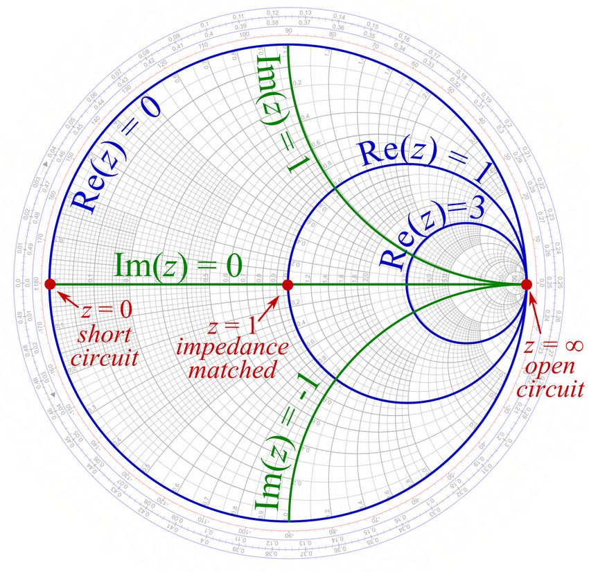
From the reflection coefficient for the different frequencies sent into the system a Smith
diagram can be made, illustrated in figure 2. From S11 it is possible to finally calculate
the Q-factor, but also the coupling coefficient of the system. One way to approximate the
Q-factor is by only looking at the amplitude difference of S11 in dB. This can be done by
2
Kurs: Självständigt arbete i teknisk fysik                    Jakob Gölén, Simon Persson

dividing the resonance frequency with the bandwidth of the resonance seen in equation 4
and illustrated in figure 1.(2)
                                         resonance f requency
                                Qtot =                                                   (4)
                                             Bandwidth

            Figure 1: Resonance frequency and Bandwidth for S11 parameters

2.2    Coupling coefficient
A system can be over, under and critically coupled. The most important thing to under-
stand is that when the system is critically coupled all of the input signal is transferred to
the system. Critical coupling is reached when the signal source has the same impedance
at resonance frequency as the system, making the coupling coefficient equal to one k = 1.
When the impedance of the source is larger than the system, over coupling is reached k > 1
and under coupling is reached when the source has a smaller impedance than the system
k < 1.(4)

2.3    The cavity and resonance frequencies
A resonance cavity does not have a defined shape though a cylindrical one is used in this
project. As described by the name it is a cavity in which resonance can be achieved and
most often it is EM-waves being sent in to the cavity. The Q-factor for cylindrical cavities

                                               3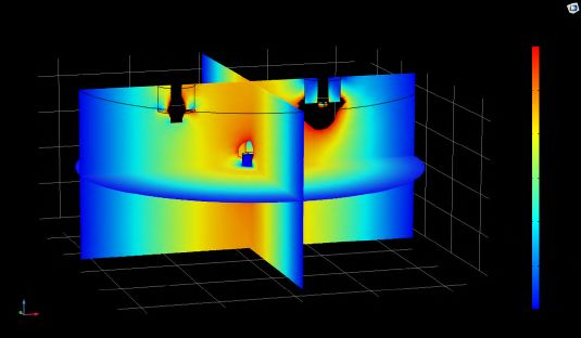
Kurs: Självständigt arbete i teknisk fysik                     Jakob Gölén, Simon Persson

                                Figure 2: Smith Diagram (6)

is affected by the impedance in the walls, the coupling points and the objects inside the
cavity.
    When thinking about resonance frequencies in a rope it is possible to have different
modes of resonances but only in one direction, while using a 3D space makes it possible to
have different modes both in overtones and in directions. Not only that but electromagnetic
waves have two parts, one electric and one magnetic, both of which affect which kind of
resonance is reached at different frequencies. When the electric waves are perpendicular
to the direction of the signal it is called transverse electric modes (T Elnm ) while transverse
magnetic mode (T Mlnm ) is for magnetic waves. lnm describes the mode in direction and
overtone of the wave. (5). For this experiment TM010 is preferred and used as seen in
figures 21 and 22 where the resonance is half a wavelength along the diameter and where
the propagation of the wave is always perpendicular to the magnetic field.

2.4    Smith diagram
In figure 2 a Smith diagram is visualised. The Smith diagram is used to help visualizing
how a signal interacts with the cavity and how the scattering change with frequency. It is
not necessary to understand exactly how the smith diagram works but a couple of details

                                               4
Kurs: Självständigt arbete i teknisk fysik Jakob Gölén, Simon Persson
from it will be discussed. First. The frequency of the signal barely changes the resistance
experienced in the system while the reactance will change, resulting in a diagram following
the same pattern as the real lines in figure 2. Secondly the resonance frequency is the
frequency closest to the point describing where the impedance (z=1) of the cavity would
match that of the signal generator. Thirdly, if the circle is larger (closer to RE(z) = 0) there
is over-coupling while there is under-coupling if the circle is smaller and does not reach
z = 1.(7)
2.5 Vector network analyser
An important tool used for this project is the vector network analyzer, normally called a
VNA. The most common VNA function is to measure scattering parameters but can also
be used to measure y-,z- and h-parameters. Only the scattering is relevant for this report.
The typical network analyzer has two ports so it can send in a signal on one side and
measure the output signal on the other end but as mentioned earlier we are only interested
in the reflected parameter meaning the signal will go in and out of the same port. When
measuring s-parameters with the VNA the signal is represented as a complex number with
its phase and amplitude.(3)
2.6 Signal generator
A signal generator is quite self explanatory. A machine that generates signals. Now there
are multiple different kinds of signal generators, some can only create normal sinusoidal
signals, some can almost create any physically possible signal given, for this project only
simple sinusoidal signals are relevant. The frequency range, maximal amplitude/power
and noise is also different for different signal generators.(8)
2.6.1 dBm
dBm is short for decibel-milliwatts and is used to avoid having to make multiple calcula-
tions when changing the strength of a signal in dB. 0 dBm is the same as one milliwatt,
from there you can convert any watt to dBm through equation 5.(9)
PmW
dBm = 10 ∗ log( ) (5)
1mW
5Kurs: Självständigt arbete i teknisk fysik Jakob Gölén, Simon Persson
2.7 Amplifier
An amplifier recieves a signal and amplifies it with a certain amount of dB. If the amplifi-
cation is 20 dB and the input signal is 10 dBm we can express the conversion as in equation
6. For the amplifier to be able to amplify the signal it needs a DC power supply.(10)
10dBm + 20dB = 30dBm = 1W (6)
One common difficulty with amplifiers is that they do not have perfect transmission
of electricity and some are lost to heat. The efficiency can be calculated by dividing the
output power by the input voltage and ampere provided by the power supply. Equation 7
shows the efficiency of the amplifier.
Pout Pout
µ= = (7)
Pin Vin Iin
2.8 Directional coupler
Directional couplers are used to redirect a specific part of a signal to the side while letting
the rest of the signal through.
Figure 3: Bi-directional coupler
Sending in a signal through port one will transport most of the signal to port two but a
defined part of the signal will exit at port three. For this project about -40 dB of the input
signal will exit through port three while the rest goes directly to port two. If instead the
signal enters through port two most will exit through port one while a small part will be
redirected to port four. In reality a non-zero amount of signal will travel from port one
to four and from port two to three but is often too small to make a real difference or is
canceled out from a mirrored signal.(11)
6Kurs: Självständigt arbete i teknisk fysik Jakob Gölén, Simon Persson
2.9 Circulator
A circulator as usually has three ports shown in figure 4. Its function is to receive a signal
through one port and sen it to the next port clockwise but not anti-clockwise. Sending a
signal into port 1 will output it to port 2, using port 2 as input will result in port 3 as output
and port 3 will send the signal to port 1.(12)
Figure 4: Clockwise circulator
2.10 Electric heating
In a normal microwave food is heated through the vibration of the dielectric properties
of water molecules in a changing electric field.(13) For graphite microplasma is instead
created and reacts with the alternating field.(14) To calculate the heating of a material
absorbing electromagnetic waves, equations with specific heat can be preformed as in
equation 8.
P∗t
∆T = (8)
m ∗ cρ
Where ∆T is the temperature difference, P is the power received by the material, t is
the amount of time the material has received the power, m is the mass of the material and
cρ is the specific heat.(15)
2.11 Comsol
Comsol is a simulation program used for complex physical simulations involving elec-
tromagnetism, magnetism, heat distribution, stress and more. It is used in this project to
validate the results from the practical tests of the real cavity. Here Comsol is used to find
resonant frequencies and values for the Smith diagram.
7Kurs: Självständigt arbete i teknisk fysik Jakob Gölén, Simon Persson
2.12 QZero
2.12.1 Purpose
QZero is a program designed specifically to extract the Q-factor from the input parameters.
It is a pretty versatile program, capable of taking S11 parameters, impedances and even
pure data from certain VNA:s as input and outputs a smith diagram as well as the Q-factor
and the resonance frequency. For this project, S11 parameters were used as input. This
required the data that was going to be used as input to be written in a table with three
columns. The first column contained the frequency at which the measurement took place.
The second column contained the real part of the S11 parameter, and the third column
contained the imaginary part of the S11 parameter.
The QZero program used in the project was a demo version, called QDEMOW. The
demo version was identical to the full version of QZero except that some features (Which
were irrelevant for this project, such as measurements of the other S-parameters, i.e. S22 ,
S21 and S12 ) were disabled and the number of data points that could be used as input were
limited to 201. This meant that after measurements had been done with the VNA-machine
or within Comsol, only the 201 data points closest to the resonance frequency should be
used and the rest of the data points had to be discarded. Otherwise, the computational
steps and the output from the program was the same as the full version(16).
2.12.2 Inner workings
The QZero software works in the following way.
First, it looks at the S11 parameter from the measurements. It then tries to fit the data
to the following mathematical formula:
a1t + a2
S11 = (9)
a3 t + 1
f − fL
t =2 (10)
fL
where fL is the loaded resonance frequency, which QZero defines as the frequency
with the smallest magnitude of the S11 parameter, and a1 , a2 and a3 are three unknown
complex coefficients. If there are many measurement points (which there are when QZero
is used in this project, since typically around 200 measurement points were used) it leads
to an over-determined system, since there are only three unknowns. The three unknown
coefficients can then be determined with the least-square method. (7)
8Kurs: Självständigt arbete i teknisk fysik Jakob Gölén, Simon Persson
When the data has been fitted to equation 9, the S11 parameters displayed in a Smith
chart form a circle. The diameter of this circle can be determined by the three found
complex coefficients:
a1
d = |a2 − | (11)
a3
When the diameter of the circle is known, the coupling coefficient is given by
d
κ= (12)
2−d
The coupling coefficient is the ratio of the external conductance (i.e. the conductance
in the connections to the cavity resonator) and the conductance in the cavity resonator.
From the a3 coefficient, the loaded Q-factor, which is the Q-factor that includes coupling
losses due to the coupling structure to and from the cavity(17), is given (7) by taking the
imaginary part of the a3 coefficient.(18)
Lastly, the unloaded Q-factor, which is the Q-factor due to losses inside the cavity
resonator (17) and which is the Q-factor which is of interest to this project, is given by:
Q0 = QL (1 + κ) (13)
2.12.3 Error estimation
While the QZero software determine the three unknown coefficients, since the system is
overdetermined the software also calculates the standard deviation σ of the three coeffi-
cients. To determine the standard deviation of the unloaded Q-factor, many steps are taken.
Firstly, the standard deviation of the loaded Q is calculated by the software as:
q
σ (QL ) = (Re(a3 ))2 + σ (a3 )2 (14)
Re(a3 ) means the real part of the a3 coefficient and σ (a3 ) is the standard deviation of
a3 . Next, the program calculates the standard deviation of the circle in the smith diagram
which it tries to fit the data to.
s
σ 2 (a1 ) a
2 (a ) + | 1 |2 σ 2 (a )
σ (d) = + σ 2 3 (15)
|a3 |2 a3
When the standard deviation of the diameter of the Q circle has been calculated, the
program moves on to calculate the standard deviation of the coupling coefficient from
9Kurs: Självständigt arbete i teknisk fysik Jakob Gölén, Simon Persson
σ (d).
2
σ (κ) = σ (d) (16)
(2 − d)2
Finally, the program uses σ (QL ) and σ (κ) to find the standard deviation of the un-
loaded Q-factor.
q
σ (Q0 ) = (1 + κ)2 σ 2 (QL ) + Q2L σ 2 (κ) (17)
(18)
However, with this method, it is only possible to describe the random error due to
fitting the S11 parameter according to equation 9. It is not possible to know any possible
systematic error due to the VNA itself.(7) The systematic error is minimized or eliminated
if the VNA is calibrated correctly.
10Kurs: Självständigt arbete i teknisk fysik Jakob Gölén, Simon Persson
3 Method
3.1 Material
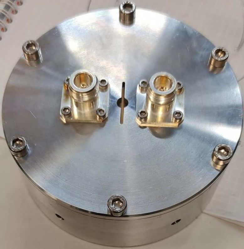
A large part of the project was doing different measurement with a cylindrical cavity res-
onator. The cavity consisted of a hollow aluminium cylinder with a detachable lid held
together with six screws to the main body. The resonator had two ports which could be
used to connect a VNA-machine to the cavity in order to do measurements of the scatter-
ing parameters. The cavity had one hole in the center of the lid used to insert material into
the cavity and three holes were fitted on the side of the main body, one of which could be
used to let a pyrometer measure the temperature inside the cavity resonator. Every part of
the cavity resonator were measured and a blueprint was created.
Figure 5: The cavity used in the project
11Kurs: Självständigt arbete i teknisk fysik Jakob Gölén, Simon Persson
Figure 6: Blueprint of the cylindrical cavity, as well as some measurements of the pyrom-
eter
12Kurs: Självständigt arbete i teknisk fysik Jakob Gölén, Simon Persson
3.2 Measurements of material
The first experiment that was done with the cavity resonator was to measure how different
materials affected the resonance frequency and the Q-factor inside the cavity. In order
to measure the scattering parameters a VNA (FieldFox RF Analyzer N9912A) was used,
which can measure scattering parameters for up to 4 GHz. The VNA was set to display
the S11 parameter in dB along the y-axis and the frequency domain along the x-axis.
Firstly, an approximation of where the resonance frequency was located was made by
visually looking on the VNA display. At the resonance frequency, a drop of dB occur
which can be seen as a pit in the graph. A good example of this can be seen in figure
15. The resonance frequency was determined to be around 2.46 GHz, so the VNA was set
to measure frequencies from 2 GHz to 3 GHz with 401 measurement points. When the
range of the VNA had been set, the VNA was calibrated by attaching an open standard,
a short standard and a load standard to the output cable of the VNA. When the VNA had
been calibrated, the output cable was connected to the port of the cavity. Extra caution
was made to ensure the cable was attached tightly to the cavity, to minimize losses. The
measurements then began. The desired material that was to be measured was placed in
the cavity, and the lid was screwed on tight. For each material, the resonance frequency
was noted. Then the bandwidth was determined by finding where the magnitude of the
S11 parameter differed by 3dB from the magnitude at the resonance frequency. The Q-
factor could then be calculated using equation 4. The results of these measurements are
presented in table 1.
3.3 Accurate measurements
After the measurements had been done, it was found that the calibration of the VNA
machine had been unsatisfactory. New measurements therefore had to be done. New,
better calibration tools from a calibration kit was used and the calibration was double
checked so that the magnitude of the S11 -parameter was as close to 0 dB as possible far
away from the resonance frequency. The range was also reduced to 2.4-2.5 GHz and the
number of measurement points were increased to 1601 points.
This time, the measurements were focused on a single material: graphite. The graphite
used was in powder form. It was placed in a glass tube which had an inner diameter of
4 mm. The glass tube was then manually inserted into the hole in the top of the cavity
resonator, and held so that the graphite was located close the middle of the empty space
inside the cylindrical cavity.
Instead of noting down the resonance frequency and the bandwidth, an USB stick was
inserted into the VNA. This made it possible to copy the data points measured by the VNA
directly to the USB and save the data as a CSV file. The data consisted of the frequency
13Kurs: Självständigt arbete i teknisk fysik Jakob Gölén, Simon Persson
measured, accompanied by the real and imaginary parts of the S11 parameter. The number
of data points was then reduced to 200 and the ones closest to the resonance frequency
were chosen. The data could then be imported to the QZero program, which produced the
Q-factor as well as the error for the Q-factor. The program also produced a smith chart.
The results from these measurements are presented in chapter 4.1.2.
3.4 The Pyrometer
To measure the temperature inside the cavity, a pyrometer would be used. In order to get
accurate readings a frame to lock the pyrometer in place at one of the holes in the side
of the cavity had to be designed. A model was designed in Solidworks, which consisted
of a curved edge with two holes, designed to go along the rim of the top of the cylinder
and was to be held in place with the screws that were holding the lid and the main body
together, effectively squeezing the frame between the body and the lid. The part that was
supposed to hold the pyrometer in place went down the side of the cavity and a hole the
size of the pyrometer was used to screw the pyrometer into the holder and hold it in place.
The model was printed using a 3D-printer and was made of plastic. The holder can be
viewed in figure 7.
Figure 7: The 3D printed holder for the pyrometer
Next, a power supply was needed to power the pyrometer, for this, an extension cable
for a 2.1 mm DC plug was used and electric tape was used to squeeze the cable with the
help of a screw at the input of the pyrometer, effectively holding it in place. The cable was
14Kurs: Självständigt arbete i teknisk fysik Jakob Gölén, Simon Persson
then cut, and the ground and live wire was connected to each respective connector. The
power supply connection can be seen in 8 and the finished setup in figure 9.
Figure 8: The connection of the power
supply to the pyrometer, which can be Figure 9: The finished setup, with the pyrom-
seen in the left hand side of the picture eter connected to the cavity
3.5 The heating experiment
The heating experiment consisted of a signal generator, connected to an amplifier. The
amplifier connects to a circulator where the signal goes through port one to two into port
one of a bi-directional coupler. Port three of the coupler was then connected to a power
meter and the cavity or resistance was connected to port two, the ports being defined as in
fig 3 and 4. The amplifier amplified the input signal and the predicted output was specified
in the data sheet (19). Since -40dB of the input signal exited through port 3, the power
meter was configured such that it displayed +40dBm in relation to its actual measurement,
effectively making it approximate the power that exited through port 2.
For the first part of the experiment, the coupler was connected to a load instead of the
cavity. The power from the signal generator and the power from the power meter was
noted for a variety of different inputs. For a few inputs the current and voltage at the input
to the amplifier was measured as well to get the efficiency of the amplifier.
For the second part the cavity was connected to the circuit. A VNA machine measured
the resonance frequency and the signal generator was set to oscillate at the resonance
frequency. About 50 mg graphite was inserted into the cavity inside a glass tube. Unfor-
tunately it became clear that the pyrometer would be of no use since it begins measuring
temperatures at 490◦ C, which was never reached. Instead a handheld electrical thermome-
ter measured the temperature of the graphite as it was pulled out of the cavity. Since
15Kurs: Självständigt arbete i teknisk fysik Jakob Gölén, Simon Persson
Figure 10: The experiment setup. The important components are a signal generator(1),
an amplifier(2), a circulator(3), a directional coupler(4), a power meter(5), drain and gate
voltage for the amplifier(6 & 7), VNA(8) and a resistance(9)
the power provided to the graphite as well as the duration, the energy was known, which
made it possible to make a prediction of what temperature was expected. This was then
compared to the actual temperature obtained in the experiment.
Figure 11: The cavity with the graphite inserted in a glass tube
16Kurs: Självständigt arbete i teknisk fysik Jakob Gölén, Simon Persson
3.6 Comsol
Three different simulations was made using Comsol to help with analyzing and predicting
the behaviour of the Q-factor and resonance of the cavity. All the simulations used one
port to send the signal into the cavity with the second port disconnected, making it just
a piece of copper inside a cavity. The first two simulations was to investigate if the tests
from the VNA on the empty cavity matches up with the simulations and vice versa. For
the first simulation all the walls of the cavity had perfect conductance where only the input
port was set to have an impedance reflecting the properties of the built in copper material,
while the second simulation used impedance properties for every part of the model. The
walls of the cavity are set to aluminum, the port is set to copper and the plastic around the
port is set as PEEK100. The third simulation also added a cylinder made of graphite in
the middle of the cavity to represent the graphite powder in the real experiment and tried
a couple of different properties for the graphite material. This is then compared to the test
with the VNA on cavity with graphite powder. In figure 12 the cavity walls is 1, where the
signal leaves the port is 2, the signal is generated in 3, the plastic surrounding the port is 4
and the graphite is 5.
Figure 12: Cavity from Comsol with graphite in center
17Kurs: Självständigt arbete i teknisk fysik Jakob Gölén, Simon Persson
Table 1: Q factor, resonant frequency and bandwidth of different materials, measured with
VNA
Material Resonant frequency [GHz] Bandwidth [Ghz] Q0
Empty Cavity 2.46428 2.46403 - 2.46453 4917
Cardboard 2.4227 2.41949 - 2.42536 413
Cloth 2.36559 2.33876 - 2.38414 52
Rubber (ball of rubber bands) 2.379272 2.37884 - 2.37970 2756
Plastic lid (from soda bottle) 2.44197 2.4414 - 2.4425 2365
Plastic lid filled with graphite 2.3849 2.3805 - 2.3884 302
Plastic lid filled with water 2.2072 - -
4 Results and Discussion
4.1 Results
4.1.1 Material study
Table 1 presents the results from the measurements of the different materials tested. The
lack of data for bandwidth and Q-factor for water is due to the type of calculations done in
order to determine the Q-factor. For this experiment, the Q-factor was determined by the
ratio between the resonance frequency and the bandwidth. For the measurements of water
however, the bandwidth could not be determined since the magnitude of the S11 parameter
never differed by 3 dB or more compared to the magnitude at the resonance frequency. A
theory for this behaviour is that it is possible that the plastic lid was filled with too much
water, which increased the effect it had on the Q-factor to the point that it was too small to
be measured.
4.1.2 Measurements with the VNA and in Comsol
Table 2: Measurements with the VNA and in Comsol, obtained with QZero
Measurement Resonant frequency [GHz] Q0 κ
Empty Cavity (VNA) 2.463 3208.1± 82.3 11.987 ± 0.331
Graphite (VNA) 2.436 299.2 ± 40.6 1.006 ± 0.262
Empty Cavity (Comsol without impedance) 2.454 3341.2 ± 255.5 11.842 ± 0.978
Empty Cavity (Comsol with impedance) 2.455 2624.1 ± 153.2 9.587 ± 0.614
Graphite (Comsol without impedance) 2.448 2571.9 ± 86.2 9.427 ± 0.347
The empty cavity is overcoupled which can be seen in the smith chart in figure 14, and
is closer to an open circuit than is ideal which leads to more of the signal being reflected.
18Kurs: Självständigt arbete i teknisk fysik Jakob Gölén, Simon Persson
S11 of the empty cavity measured with the VNA
0.5
0
-0.5
S11 [dB]
-1
-1.5
-2
2.4 2.41 2.42 2.43 2.44 2.45 2.46 2.47 2.48 2.49 2.5
Frequency [Hz] 109
Figure 14: Measured S11 of the empty
Figure 13: Measured S11 (in dB) of the empty cavity with the VNA, presented in a
cavity with the VNA Smith-chart
S11 of the cavity when graphite was inserted, measured with the VNA
0
-5
-10
S11 [dB]
-15
-20
-25
-30
2 2.1 2.2 2.3 2.4 2.5 2.6
Frequency [Hz] 109
Figure 16: Measured S11 of the cavity
Figure 15: Measured S11 (in dB) of the cavity when graphite was inserted, measured
when graphite was inserted, measured with with the VNA and presented in a Smith-
the VNA chart
19Kurs: Självständigt arbete i teknisk fysik Jakob Gölén, Simon Persson
This is also supported by the high coupling coefficient from table 3. This changes when
the graphite is inserted. The system then gets critically coupled since the system matches
the impedance of the signal source, which can be seen in figure 16. This leads to mini-
mal losses of reflection at the resonance frequency, which can be seen by comparing the
magnitude of figure 13 and 15.
S11 (in dB) of the empty cavity, simulated in Comsol
0
-0.5
-1
S11 [dB]
-1.5
-2
-2.5
-3
2.42 2.43 2.44 2.45 2.46 2.47 2.48
Frequency [Hz] 109
Figure 18: Measured S11 of the empty
Figure 17: Measured S11 (in dB) of the empty cavity simulated in Comsol, presented in
cavity, simulated in Comsol a Smith-chart
The empty simulated cavity seems to match the actually empty cavity pretty well.
They both are within the same margin of error for both the Q-factor and the coupling
coefficient. The simulation with graphite does not seem to match the actual cavity with
graphite. Though there is a decrease in the Q-factor and the coupling coefficient is slightly
better, it is not nearly on the same level as the actual cavity.
The colors in figure 21 and 22 describe the strength of the electric field inside the cav-
ities and its field pattern matches that of the T M010 mode described in the theory section.
The signal is sent from the left coupler in both pictures.
4.1.3 Amplification and efficiency of amplifier
From these values it is possible to calculate the efficiency for the amplifier through equa-
tion 7, resulting in µ = 25dBm 0.3W
17.3W ≈ 17W ≈ 2% for the output of 0.3W and µ = 48W ≈
34dBm
2.5W
48W ≈ 5% for the output of 2.5 W.
20Kurs: Självständigt arbete i teknisk fysik Jakob Gölén, Simon Persson
S11 (in dB) of the cavity when graphite was inserted, simulated in Comsol
0
-0.5
-1
S11 [dB]
-1.5
-2
-2.5
-3
2.43 2.435 2.44 2.445 2.45 2.455 2.46 2.465 2.47 2.475
Frequency [Hz]
Figure 20: Measured S11 of the cavity
Figure 19: Measured S11 of the cavity when when graphite was inserted, simulated in
graphite was inserted, simulated in Comsol Comsol and presented in a smith chart
Figure 21: Simulation without graphite Figure 22: Simulations with graphite
Table 3: amplification and power input to amplifier
input signal [dBm] output signal [dBm] input power [W]
-20 -23 –
-5 -14 –
0 -6 –
5 9 –
10 25 17.3
13 34 48
21Kurs: Självständigt arbete i teknisk fysik Jakob Gölén, Simon Persson
4.1.4 Heating of graphite
Using the specific heat of graphite from equation 8 the temperature difference at 33dBm
or 2 watt for half a minute, where no energy is dissipated from the graphite is 1700◦ C.
This is compared to the actual temperature measured 30 seconds after the signal had been
shut down at 100◦ C.
4.2 Discussion
4.2.1 Material study
The measurements done in a material study gave a hint of how much microwaves affect
the material. Plastic and rubber was affected very little, but the microwave had a huge
impact of the water, which is to be expected due to the dipole nature of water.
4.2.2 VNA and Comsol measurements obtained by QZero
The accurate measurements done on the actual cavity and in Comsol are interesting. The
first simulation with mostly perfect conductivity gave a result which almost perfectly re-
flects the results from the VNA on the empty cavity, when adding impedance to the rest of
the cavity the result of the Q-factor is still close to that of the real experiment but further
from perfect. Why this is the case is not clear but may have to do with how the materials in
Comsol does not represent the real materials correctly. The simulations of graphite gave
unexpected results, only slightly lowering the Q-factor while the real experiment had a
significant change of quality factor and resonance frequency. The leading theory for the
discrepancy is that there was some error when choosing the material. There were many
different kinds of graphite to choose from and there may be some important properties of
graphite that is not set in the basic materials already part of Comsol. Even if multiple dif-
ferent properties was change and added no noticeable difference where observed. Another
likely error with the simulation is simply that there was an error with the setup. Comsol is
a very complex program and it took many hours to even get a decent result with the empty
cavity, so it’s not out of the question that some setting or boundary condition was wrongly
defined.
4.2.3 Heating experiment
When the output power from the amplifier goes over one Watt the temperature of the
amplifier rise up to 200◦ C with the simple setup of a small fan and heat sink. When
looking at the data sheet for the used amplifier we can see that the resulting efficiency of
22Kurs: Självständigt arbete i teknisk fysik Jakob Gölén, Simon Persson
2-5% is not too far off since the amplifier is built for much higher powers than those used
here. This can be seen in figure 3 in the datasheet, which shows an efficiency of 30% for
an output of 50 watts, and the output is around 2 watts for this experiment, leading to an
even worse efficiency(19). The heat resulting in the graphite is significantly lower than
the 1700◦ C that it would have been if there was no emission from the tube with graphite,
making us believe that the temperature found an equilibrium at around 100-150◦ C or that
the resonance frequency had such a significant change that most of the signal was reflected
back to the circulator and out to thin air. As the setup was now it was impossible to
measure the heat of the cavity as it was heated up, since the graphite had to be placed on
the bottom om the cavity instead of being held in the middle, since the holes for measuring
the temperature is placed at the middle of the cavity walls.
5 Conclusion
The four goals have been fulfilled. Knowledge about Q-factors and resonance frequencies
have been obtained and the empty cavity has been measured to have a Q-factor of around
3200 and a resonance frequency at 2.46 GHz. Measurements in Comsol seemed to match
the real cavity when it was empty with perfect conductivity, but there was a discrepancy
when it was simulated with graphite and when proper impedances was set to the walls,
which is discussed in the report. The experiment was also done, and the pyrometer was
fitted and ready to do measurements, unfortunately it was not used. The efficiency of the
amplifier was calculated and the microwaves managed to heat the graphite to 100-150◦ C.
This was much lower than the theoretical temperature that could have been used with the
energy provided, and was also mentioned in the discussion.
5.1 Whats next?
The end goal with the experimental setup is, one, to be able to measure the change of
Q-factor, coupling and resonance frequency, two, to change the frequency sent from the
signal generator as the resonance frequency is changing with the heating. To do this the
signal generator is supposed to send frequency sweeps every couple of seconds and then
reflection parameters can be measured through the third end of the circulator as the signal
is reflected from the cavity and compared to the signal coming out from the third port of
the directional coupler. With this it is possible to automatically change the frequency of
the signal generator to match the changed resonance of the cavity.
To avoid overheating with higher power it may be good to change the amplifier for one
that has a better efficiency for lower power levels. Quartz wool has been bought and can
23Kurs: Självständigt arbete i teknisk fysik Jakob Gölén, Simon Persson
be used to make sure the graphite is placed in the middle of the cavity by filling half of
the glass/quartz tube along the center axis of the cavity. The tube is shown in figure 11.
When the graphite has been placed in the middle more tests with higher power needs to
be conducted to see if it is possible to reach higher temperatures without needing to adapt
the frequency of the input signal. It is still interesting to look at the changing reflection
parameter to understand the interaction of graphite or other materials with high intensity
microwaves.
24Kurs: Självständigt arbete i teknisk fysik Jakob Gölén, Simon Persson
6 References
[1] Jones DA, Lelyveld TP, Mavrofidis SD, Kingman SW, Miles NJ. Microwave heating
applications in environmental engineering — a review. Resources, Conservation and
Recycling. 2002;34(2):75–90.
[2] Green EI. The Story of Q. American Scientist. 1955;43(4):584–594.
[3] Ballo D. Network Analyzer basics. Hewlett-Packard Company; 1997. Accessed:
2021-05-19. http://maxwell.sze.hu/˜ungert/Radiorendszerek_
satlab/Segedanyagok/Szoftver/Agilent_Modulation/Data/
pdf/nabas.pdf.
[4] Pozar DM. Microwave Engineering -4th ed. 111 River Street, New York, USA: John
Wiley & Sons, Inc.; 2011.
[5] Understanding TEM, TE, and TM Waveguide Modes. Mi-
Wave;. Accessed: 2021-05-20. https://www.miwv.com/
understanding-tem-te-and-tm-waveguide-modes/.
[6] Sbyrnes321. Smith chart explanation. Wikimedia; 2018. Accessed: 2021-
05-19. https://commons.wikimedia.org/w/index.php?curid=
20319450.
[7] Kajfez D. QZero for Windows. Oxford, Mississippi, USA; 2001.
[8] What is a Signal Generator: different types. Electric Notes;. Ac-
cessed: 2021-05-19. https://www.electronics-notes.
com/articles/test-methods/signal-generators/
what-is-a-signal-generator.php.
[9] Decibel-milliwatt. RapidTables;. Accessed: 2021-05-20. .
[10] Crecraft D, Gorham D. Electronics -2nd ed. CRC Press; 2003.
[11] Microwave Engineering - Directional Couplers. Tutorials Point;. Accessed: 2021-05-
20. https://www.tutorialspoint.com/microwave_engineering/
microwave_engineering_directional_couplers.htm.
[12] Circulators. Microwaves 101;. Accessed: 2021-05-20.
https://www.microwaves101.com/encyclopedias/circulators.
25Kurs: Självständigt arbete i teknisk fysik Jakob Gölén, Simon Persson
[13] How does a microwave heat water and will the water blow up in my face?. the In-
ternational Association for the Properties of Water and Steam; 2013. Accessed:
2021-05-20. http://iapws.org/faq1/mwave.html.
[14] Chandrasekaran S, Basak T, Srinivasan R. Microwave heating characteristics of
graphite based powder mixtures. Chennai, India: Department of Chemical Engi-
neering, Indian Institute of Technology Madras; 2013. 600 036.
[15] Szyk B. Specific Heat Calculator. Omni calculator; 2021. Accessed: 2021-05-
20. https://www.omnicalculator.com/physics/specific-heat#
heat-capacity-formula.
[16] Kajfez D. QDEMOW; 2001. Accessed: 2021-04-01. https://people.
engineering.olemiss.edu/darko-kajfez/software/.
[17] Hosseini SE, Karimi A, Jahanbakht S. Q-factor of optical delay-line based cavities
and oscillators. Optics Communications. 2017;407(1):349–354.
[18] Kajfez D. Data Processing For Q Factor Measurement. In: 43rd ARFTG Conference
Digest. ARFTG. San Diego, California, USA: IEEE; 1994. p. 104–111.
[19] BLC2425M9LS250 - Power LDMOS transistor. Nijmegen, Netherlands; 2016.
26You can also read