Rainfall-runoff modeling using adaptive neuro-fuzzy inference system (ANFIS) and genetic algorithm (GA)
←
→
Page content transcription
If your browser does not render page correctly, please read the page content below
© 2022 The Authors                                                                    Water Supply Vol 22 No 10, 7460 doi: 10.2166/ws.2022.318

              Rainfall–runoff modeling using adaptive neuro-fuzzy inference system (ANFIS)
              and genetic algorithm (GA)

              Shabnam Vakili              * and Seyed Morteza Mousavi
              Water Resources Group, Department of Civil Engineering, K.N Toosi University of Technology, No. 1346, Vali Asr Street, Mirdamad Intersection, Tehran
              1996715433, Iran
              *Corresponding author. E-mail: vakili_c@ahoo.cm, shabnamvakili63@gmail.com

                  SV, 0000-0003-0136-1118

              ABSTRACT

              Nonlinear properties and natural uncertainties in the rainfall–runoff process, the necessity of extensive data, and the complexity of the phys-
              ical models have caused researchers to use methods inspired by nature such as artificial neural networks, fuzzy systems, and genetic
              algorithms (GA). The main purpose of this study was to estimate runoff employing Adaptive Neuro-Fuzzy Inference System (ANFIS) and
              GA models using accessible, applicable, and easily available climatic data. The results of the two models were compared to provide an
              easy but reliable model to estimate evaporation. The models were utilized to estimate the runoff in Sivand river basin located in Fars province
              in central Iran. The results were compared considering a range of model performance indicators as mean absolute error (MAE), Nash–Sutcliffe
              efficiency coefficient (NSE), root mean square error (RMSE), and correlation coefficient (R2). According to the results presented, ANFIS with
              lower RMSE and MAE and higher correlation coefficient and NSE between the observed and predicted values provided higher accuracy in
              comparison to GA. Also, it was clear that using ANFIS, an increase in the number of membership functions and running cycles of the
              model decreased the error such that the results in the studied stations using were improved by 42, 44 and 11%, respectively by increasing
              the number of membership functions and run rounds. Also, it was observed that the nonlinear models performed better than the linear
              models when applying GA such that non-linearizing the model improved the results of the GA model in the three studied stations by
              27.5%, 17%, and 9.5%, respectively. Meanwhile, considering RMSE amounts the best results from ANFIS were 23%, 54.6%, and 35.7%
              better than the best results from GA in the three stations, respectively. According to the results of the study runoff can be estimated appro-
              priately by utilizing ony meteorological data and there is no need for more complex and interdependent data. A sensitivity analysis was
              conducted too by removing rainfall and evaporation parameters in two different scenarios. The ANFIS model showed the lowest sensitivity
              to the absence of those parameters especially evaporation in scenario 3 with RMSE ¼ 0, 0, and 0.005 for Chambian, Dashtbal, and Tang
              Balaghi stations, respectively. The results of the study justifies using ANFIS employing only meteorological data to estimate runoff in areas
              when scant data are available.

              Key words: adaptive neuro-fuzzyi Inference system (ANFIS), genetic algorithm (GA), modeling, rainfall–runoff relations

              HIGHLIGHT

              •   In this study, the effect of meteorological parameters on runoff estimation was investigated with different membership functions and
                  rounds of ANFIS in an adaptive fuzzy neural inference system (ANFIS) and linear and nonlinear models in the genetic algorithm (GA).
                  To the best of our knowledge, a study of the number of membership functions and rounds of ANFIS and the linearity and nonlinearity
                  of the GA model using minimal meteorological data is a novel endeavor. Most researchers have focused on complex physiographic charac-
                  teristics, which are difficult to access, while according to the results of this study runoff these can be estimated appropriately by utilizing
                  minimum meteorological data. Also, as it is explained in the “sensitivity analysis” section, reliable results can be obtained by using ANFIS
                  even after removing the evaporation parameter from the input data.

              This is an Open Access article distributed under the terms of the Creative Commons Attribution Licence (CC BY 4.0), which permits copying, adaptation and
              redistribution, provided the original work is properly cited (http://creativecommons.org/licenses/by/4.0/).

Downloaded from http://iwaponline.com/ws/article-pdf/22/10/7460/1127079/ws022107460.pdf
by guest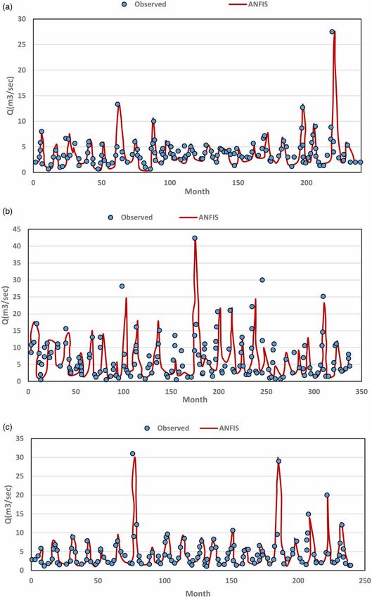
Water Supply Vol 22 No 10, 7461

                     GRAPHICAL ABSTRACT

                     INTRODUCTION
                     The estimation of water availability plays an important role in planning water resource projects. Also, the prerequisite for any
                     watershed development plan is understanding the hydrology of the watershed and determining runoff yield. The first step in
                     the estimation of water availability is the computation of runoff resulting from rainfall on river catchments.
                       Existence of numerous effective parameters in the process of converting rainfall to runoff along with high complexities and
                     nonlinear relationships among those parameters have made it very difficult to accurately predict the amount of runoff caused
                     by rainfall. Also, the inputs and outputs from watershed systems have very important roles in predicting the amount of runoff.
                     Many attempts have been made to estimate the runoff amount in a catchment caused by rainfall. However, the results were
                     not very satisfactory due to the abovementioned reasons. Therefore, the researchers found intelligent neural systems to be
                     useful tools and turned to nature-inspired methods such as Artificial Neural Networks (ANN), ANFIS, and GA. Moreover,
                     saving time and money caused the use of the abovementioned intelligent methods to seem necessary, especially in catchments
                     with few or no hydrometric and meteorological stations. As such, many researchers have employed intelligent methods in
                     studying the complicated process of the production of runoff by rainfall in recent years.
                       Ghose et al. (2013) used ANFIS and GA to predict and optimize the amount of runoff. As the first phase of the study, they
                     developed runoff rating curves considering the present-day water level (H(t)) as the input and the present-day runoff (Q(t)) as
                     the output of the model. They developed the Non-Linear Multiple Regression (NLMR) technique using ANFIS model. Later,
                     they coupled GA with NLMR to obtain the hydrological parameters which made the runoff maximum. Suparta & Samah
                     (2020) used the ANN method and the analyses of six-year rainfall data on a monthly basis in South Tangerang City. They
                     found the rainfall prediction based on ANFIS time series promising where Mean Absolute Percentage Error (MAPE) was
                     below 20%. Zhihua et al. (2020) studied the runoff increase in a basin due to vegetation degradation. They used SWAT
                     and ANN models and an improved metaheuristic model. Considering the results and according to the regression model,
                     the points’ distribution in Soil and Water Assessment Tool-Multi-Layer Perceptron/Modified Whale Optimization Algorithm
                     (SWAT-MLP/MWOA) model had the best linear fit. According to the values obtained from statistical indices, the SWAT-
                     ANN model seemed better than the SWAT model and presented itself as the best model for runoff prediction. Nath et al.
                     (2020) used the modified ANFIS, estimated the runoff, and compared the results to those from Auto Regressive Integrated
                     Moving Average (ARIMA) model. They concluded that the proposed Particle Swarm Optimization-ANFIS (PSO-ANFIS)
                     model performed better than ARIMA and conventional ANFIS regarding the accuracy of the runoff prediction. Kan et al.
                     (2020) proposed a novel Hybrid Machine Learning (HML) hydrological model to forecast flooding by coupling ANN with
                     the K-nearest neighbor (KNN) method. A GA and Levenberg–Marquardt-based multi-objective training method was also pro-
                     posed in order to overcome the number of local minimums which appear using the traditional neural network training. The
                     satisfactory performance and reliable stability of the HML hydrological model was indicated by its real-world applications,
                     crystalizing the possibility of further applications of the HML hydrological model in flood forecasting studies.
                       A novel Biogeography-Based Optimization (BBO) algorithm was adopted by Roy et al. (2019) using ANFIS. They named it
                     BBO-ANFIS and used it for one day ahead of runoff forecasting. They also checked the robustness of the BBO-ANFIS model
                     within a comparative study with two well known hybrid models of GA-based ANFIS (GA-ANFIS) and firefly-based ANFIS
                     (FA-ANFIS). According to the results, the BBO-ANFIS model had a better performance than both the GA-ANFIS and the FA-
                     ANFIS models in rainfall–runoff (R-R) modeling. Kumanlioglu & Fistikoglu (2019) simulated a daily rainfall–runoff model by
                     integrating ANN and GA. They carried out the integrations on the daily rainfall–runoff model Génie Rural à 4 paramètres
                     Journalier (GR4 J) which is a catchment water balance model relating runoff to rainfall and evapotranspiration using daily
                     data. Results showed that the hybrid model led to a better prediction than both the original GR4 J model and the single
                     ANN-based runoff prediction model. Morales et al. (2021) simulated rainfall–runoff with a Self-Identification Neuro-Fuzzy
                     Inference Model (SINFIM). According to their results, the proposed model was a solid alternative to forecasting the

Downloaded from http://iwaponline.com/ws/article-pdf/22/10/7460/1127079/ws022107460.pdf
by guest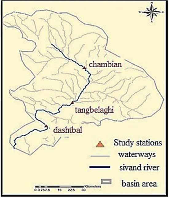
Water Supply Vol 22 No 10, 7462

              runoff in a given watershed, obtaining good measurements, managing to predict both the low and the peak runoff values from
              rainfall events, avoiding the necessity of determining the lags in both time series and number of fuzzy rules.
                 Talei et al. (2010) used ANFIS for event-based rainfall–runoff modeling. They compared the results to an established phys-
              ical-based model. According to the study results, ANFIS was comparable to the physical model and gave a better peak flow
              estimation than the physical model. Dorum et al. (2010) studied the rainfall–runoff data using ANN and ANFIS models. They
              used a multi-regression (MR) model and compared the results obtained from ANN and ANFIS to the results from MR tra-
              ditional methods. According to the study results, ANN and ANFIS models could be used to determine the rainfall–runoff
              relationship in Susurluk Basin in all cases except peak situations.
                 Asadi et al. (2013) used GA to evolve the weights of the neural network employed to model rainfall–runoff process. They pre-
              processed the data-by-data transformation, selection of input data, and data clustering to improve the accuracy of the model
              prediction. They found that a faster training, a higher degree of accuracy, and a better adaptation of nonlinear functional relation-
              ship between rainfall and runoff were achieved by adopting this methodology. The ANN and Ensemble neural networks (ENN)
              models were compared to each other by some other researchers including Kumar et al. (2019) to estimate the rainfall–runoff
              relationship. They suggested ENN models as a superior approach for rainfall–runoff modeling. The impact of changes in climate
              parameters on river runoff, and consequently, on hydropower generation was analyzed by Tayebiyan et al. (2019). They concluded
              that the output of the hydropower reservoir system is highly dependent on the river runoff, and in turn, on climate parameters. As
              such, the reservoir operators/managers should consider the impacts of the change in climate parameters to secure water supplies.
              The application of ANN and fuzzy logic and GA in rainfall–runoff relationships was introduced by Chandwani et al. (2015). It
              partially replaced time-consuming conventional mathematical techniques with time-saving computational tools.
                 A hybrid method that combined a parallel GA model with a fuzzy optimal model in a cluster of computers was developed
              by Cheng et al. (2005). Based on the comparison of the results of the serial and parallel GA models, the current methodology
              significantly reduces the overall optimization time and improves the results. Most studies estimated runoff using other models,
              benefiting the availability of recent runoff data for the studied basin and physiographic characteristics. However, a compari-
              son of membership functions and the number of run rounds in ANFIS and a comparison of linearity and nonlinearity of GA
              were not considered. In the present study, these cases were investigated. Meanwhile, although some researchers believe that
              both climatic and physiographic factors are needed to estimate runoff, according to the results of this study climatic data
              alone can offer acceptable and sufficient results using ANFIS and GA in runoff estimation. Investigating the effect of the
              number of membership functions, the number of run rounds, performing sensitivity analysis with available meteorological
              parameters, accompanied with estimating runoff using the above mentioned models and finally providing a reliable,
              simple and applicable solution for rainfall–runoff relation is one of the important achievements of this study.
                 Since the variance in our data set varies from case to case, therefore PSO-ANFIS model was not used (Nath et al. 2020).
              Meanwhile, one of the main disadvantages of the SWAT-ANN model is the need for many input parameters including soil
              data which, was not consistent with the goal of this study. In this study, only meteorological parameters were employed,
              showing that a successful rainfall–runoff analysis could be done using those methods employing only these easily accessible
              input data. Moreover, the results of some studies showed that more accurate results can be obtained from the hybrid models
              for simulating runoff in rivers if the climatic data were long enough (Zhihua et al. 2020). Therefore, to use successfully the
              hybrid models in this study climatic data for a longer time period than that was available was required. The authors hope
              it could be done in future with acquiring data for a time period which is long enough to use hybrid methods. This was men-
              tioned in the recommendations section in the revised manuscript (Lines 470–476).
                 The ANFIS and the GA models were employed to estimate the runoff in the catchment of Sivand River. Considering the
              available data precipitation, evaporation, and maximum, minimum and average temperatures were used as inputs. The cur-
              rent runoff in the river was defined as the output. The main purpose of this study was to model runoff using ANFIS and GA
              with only climatic data as input and comparing the results. The best model for estimating the runoff in the studied basin was
              selected based on the study results.

              METHODS
              The study area
              Sivand River is located between latitudes of 29⁰510 38″ up to 30⁰360 25″ north and longitudes of 52⁰460 14″ up to 52⁰530 26″ east.
              The length of the river in the studied province is about 110 km. The position of the studied stations in the basin is shown in Figure 1.

Downloaded from http://iwaponline.com/ws/article-pdf/22/10/7460/1127079/ws022107460.pdf
by guest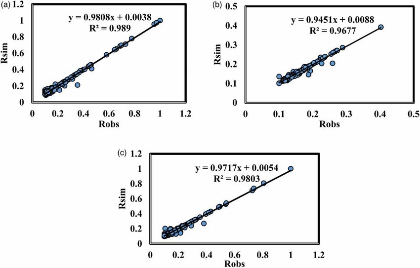
Water Supply Vol 22 No 10, 7463

                     Figure 1 | Geographical location of the stations in the study area.

                        After preparing the statistics needed to simulate runoff and reviewing them, appropriate data with a sufficient statistical
                     time period were found in the Chambian, Tangbelaghi and Dashtbal stations among the stations located in the studied
                     basin (Figure 1). The monthly data including rainfall, runoff, and also minimum, maximum, and average temperatures
                     from those three selected stations were used in the modeling. Also, there existed evaporation data for time periods of 20,
                     28 and 20 years in Chambian, Dashtbal and Tangbelaghi stations, respectively. The average meteorological data used in
                     the studied basin for the three selected stations are given in Table 1.

                     Adaptive – Neuro-Fuzzy Inference System (ANFIS)
                     Fuzzy logic has evolved as a useful approach to model the rainfall–runoff phenomenon. However, it has some degree of
                     uncertainty regarding hydrological processes. The main idea of the approach is to consider variables in a parametric uncer-
                     tain manner rather than numerically precise quantities (Ş en & Altunkaynak 2004; Moraga & Salas 2005). The neural
                     network uses training data to determine the membership functions and fuzzy rules of a fuzzy logic system in the frame of
                     a Neuro-Fuzzy system (Zahedi & Zahedi 2018).

                     Table 1 | Average long-term statistics for the selected stations

                                                                       Rainfall           Runoff   Minimum            Maximum               Average            Evaporation
                     Station           Statistical parameter           (mm)               (m3/s)   temperature (°C)   temperature (°C)      temperature (°C)   (mm)

                     Chambian          Average                         22.9               2.94     11.5               26.3                  18.9               196.7
                                       Minimum                         0                  0        3                 26.9                  5.1                11.5
                                       Maximum                         243.5              27.51    26.9               41                    33                 592
                                       Deviation from the              37.4               3.88     8                  8.9                   8.4                116.7
                                         standard
                     Dashtbal          Average                         32.13              4.7      7.7                23.1                  15.6               214.5
                                       Minimum                         0                  0        8.6               3.3                   1                 35.7
                                       Maximum                         333                42.4     22.1               40.5                  29.9               549.5
                                       Deviation from the              51.3               7        7.7                9.5                   8.2                123.6
                                         standard
                     Tangbelaghi       Average                         50                 3.7      5.5                23.1                  14.3               151
                                       Minimum                         0                  0.33     6.2               6.2                   0                  2.5
                                       Maximum                         441.5              31       17.2               36.6                  26.8               468
                                       Deviation from the              80.3               4.8      6.3                8.6                   7.4                103.5
                                         standard

Downloaded from http://iwaponline.com/ws/article-pdf/22/10/7460/1127079/ws022107460.pdf
by guest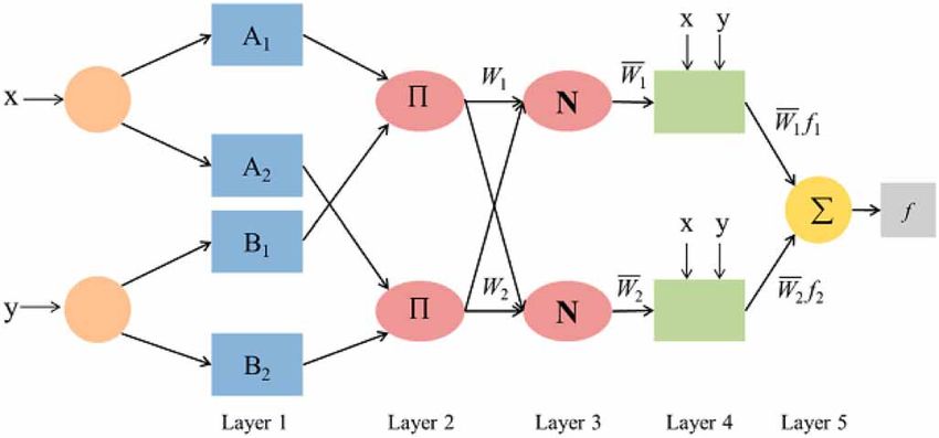
Water Supply Vol 22 No 10, 7464

                 Many Neuro-Fuzzy systems allow the application of gradient descent learning as long as differentiable membership func-
              tions are used (Nauck & Nürnberger 2013). These are based on the fuzzy structure of Takagi-Sugeno-Kang (Takagi & Sugeno
              1985). One of the first popular Neuro-Fuzzy systems is ANFIS. The model was also approved in 1991 by Jang (1993) and has
              been widely applied in rainfall–runoff modeling ( Jothiprakash et al. 2009; Ghose et al. 2013; Panchal et al. 2014; Anusree &
              Varghese 2016).
                 To model nonlinear functions, and to identify nonlinear components online in a control system and predict a chaotic time
              series, all yielding remarkable results, Tagaki & Sugeno (1985) proposed the ANFIS model. ANFIS is a combination of ANN
              and fuzzy systems using ANN learning capabilities to obtain fuzzy if-then rules with appropriate membership functions,
              which is an important advantage. These functions can learn from the imprecise input data and can yield inference capabili-
              ties. Another advantage of ANFIS is that it can provide us with a more stable training process because it can make effective
              use of self-learning and memory abilities of neural networks (Huang et al. 2017). In general, ANFIS is constructed in five
              layers as the following. The input layer is regarded as an antecedent parameter; the three hidden layers called rule-based
              layers with three constant parameters and one consequent parameter; and the output layer (see Figure 2).
                 In the first layer, an input is transformed into a degree between 0 and 1(fuzzification), which is called a premise parameter.
              It is an activation function with membership functions such as triangular, trapezoidal, Gaussian, and/or generalized bell-
              shaped functions. The second layer uses the product operator and estimates each incoming signal for each neuron. In the
              third and fourth layers, the normalization and fuzzification of all input signals are performed, respectively. Finally, in the
              last layer, all weighted output values are summarized. The input–output structure of the prediction model can be formulated
              through an equation as below (Liu 2010):

                              rffiffiffi n
                               1X
              RMSE ¼                 (y pred  yobs )2                                                                                    (1)
                               n k¼1

                According to the observation (training and testing), the input parameters in the form of meteorological data which have
              undergone a learning process, and the input–output structure of the performance of the network can be formulated through
              the correlation coefficient, R. These parameters are often defined in terms of the prediction of error, that is, the difference
              between the actual and the predicted values (Khoshnevisan et al. 2014) as below:

                vffiffiffiffiffiffiffiffiffiffiffiffiffiffiffiffiffiffiffiffiffiffiffiffiffiffiffiffiffiffiffiffiffiffiffiffiffiffiffiffiffiffiffiffiffi
                u
                u         P n
                u                (yobs  y pred )2
                u
              R¼u
                u1
                         K¼1
                                                                                                                                          (2)
                t                P n
                                        (y pred )2
                                      k¼1

              Figure 2 | Design of the ANFIS network (Jang 1993).

Downloaded from http://iwaponline.com/ws/article-pdf/22/10/7460/1127079/ws022107460.pdf
by guest
Water Supply Vol 22 No 10, 7465
where yobs presents the value of an observation, ypred shows the value of a predicted result, and n presents the data number:
1X l
MAE ¼ jYOi þ YEi j (3)
N i¼1
Mean absolute error (MAE) is used to test the fit of the model:
P
l
(YOi YEi )2
i¼1
NSE ¼ 1 (4)
Pl
2
(YOi YOi
)
i¼1
The NSE (Nash–Sutcliffe Efficiency) value is a normalized statistic of the relative scale of the residual variance (noise) com-
pared to the measured data variance (information) which is used to measure the goodness-of-fit of a model. A value closer to
one means a more accurate model. YEi denotes the ith estimated monthly runoff using a model; YOi denotes the ith observed
monthly runoff; YEi shows the average of the estimated monthly runoff; YOi presents the average of the observed monthly
runoff, and l shows the number of observations (Roy et al. 2019).
Genetic algorithm (GA)
The first and most important strength of GAs is that they are inherently parallel. Most other algorithms are not parallel and
can only search the space of the problem at a glance, and if the solution found is an optimal local solution or a subset of the
original solution, it must discard all that has already been done and start all over again. Because GA has multiple starting
points, it can search the problem space from several different directions at once. If one of the starting points fails, the
other paths will continue, and more resources will be available to them. Another strength of genetic algorithms that initially
seemed to be a shortcoming is that GAs know nothing about the problems they solve, and we call them blind watches. They
put random changes in the path of their desired solutions and then use the fit function to measure whether those changes
have made progress or not. Since its decisions are essentially random, it is theoretically open to all possible solutions to
the problem. But issues that are limited to information must be decided by analogy, in which case many new solutions are
lost. Another advantage of GAs is that they can change several parameters simultaneously. Many real issues cannot be limited
to one attribute to maximize or minimize that attribute. GAs are very useful in solving such problems and in fact their ability
to work in parallel gives them this property (Marouf et al. 2015).
Genetic algorithms are powerful optimization techniques (Holland 1975; Goldberg 1989). Those are based on the prin-
ciples of natural selection and species evolution and can work with numerical values to establish objective functions
without difficulty. They are free from a particular model structure. Therefore, their only requirement is an estimation of
the objective function value for each decision set in order to proceed, neglecting whether such information comes from a
simple equation or a very complex model (Jang & Sun 1995).
The models, which were used to estimate runoff in the studied basin and to determine its parameters by GA, are introduced
in this portion of the study. According to the existing relationship between runoff and the variables used in this study (pre-
cipitation, evaporation, the minimum, maximum, and average temperatures) the proposed models are expressed linearly and
nonlinearly to compare the estimated runoff.
Linear model
Runoff ¼ b0 þ b1 x1 þ b2 x2 þ b3 x3 þ b4 x4 þ b5 x5 (5)
where
X1: Precipitation (mm)
X2: Evaporation (mm)
X3: Mean temperature (°c)
X4: Maximum temperature (°c)
X5: Minimum temperature (°c)
b0-b5: Model coefficients
Downloaded from http://iwaponline.com/ws/article-pdf/22/10/7460/1127079/ws022107460.pdf
by guestWater Supply Vol 22 No 10, 7466
In this model, the objective function is to minimize the sum of the squares of the differences between the observed and the
predicted runoff values in the studied catchment. Therefore, using the GA optimization method, the values of the coefficients
of the linear model are determined in such a way that the error amount, which is the difference between the observed and the
simulated runoff values resulting from the use of the linear model could be minimized. The objective function is obtained
using the following equation:
X
n
Minimize e2i (6)
i¼1
e ¼ (Robs Rsim )2 (7)
where
e: Error (the difference between observed and simulated values)
Robs: Observed runoff value
Rsim: Simulated (predicted) runoff value
Non-linear model
Runoff ¼ b0 þ b1 xa11 þ b2 xa22 þ b3 xa33 þ b4 xa44 þ b5 xa55 (8)
In this model the exponents are a1–a5 and the other parameters are as defined in the previous section. By determining the
parameter values for each of the linear and nonlinear models, the runoff can be predicted. Also, by calculating the root mean
square error (RMSE) and the correlation coefficient (R2) between the observed and the predicted runoff values in each
station, the appropriate model is selected to estimate runoff in the basin.
RESULTS AND DISCUSSION
The main goal of this study was not comparing all methods with each other. Obviously, each model has its own advantages
and disadvantages. As it was mentioned in the literature review, although many researchers expressed their positive attitude
about using ANFIS and GA, those methods were not used solely by employing precipitation, temperature, and evaporation.
In this study, only these meteorological parameters -which could be acquired easily- were employed, showing that a successful
rainfall–runoff analysis could be done using those methods employing only these easily accessible input data.
The runoff amount in the stations located in the Sivand river basin was estimated. Using MATLAB, different models of
ANFIS and GA were created for each of the chosen stations in the basin. The better model was selected after estimating
the runoff amounts using the models and comparing them to the observed amounts and calculating the correlation coeffi-
cients (R2) and the RMSE. The results of modeling by ANFIS are summarized below.
Five models in Chambian station, eight models in Dashtbal, and four models in Tangbelaghi stations were used to simulate
runoff amounts. The results are presented in Table 2.
By analyzing the results and observing Table 2 and Figures 3 and 4 provided by the selected models in the chosen stations, it
was concluded that increasing the number of input membership functions and using the linear output membership function
instead of a constant one significantly improves the results of the models. However, the use of a large number of membership
functions (more than 4) makes the calculation process longer, which is not desired in the simulation and modeling of hydro-
logical phenomena. In fact, as the number of cycles increased, the computation time increased by approximately 25%. The
number of membership functions 3, 4, 5 and 6 were examined for Dashtbal station in both linear and constant models. As can
be seen in Table 2, when the number of membership functions is 4, the amount of model error decreases significantly, but
beyond this, the number of model errors does not differ much, so there is no need to increase the number of these functions
and increase the time. Therefore, two other stations with the same number were surveyed. The Investigation of the results by
model evaluation criteria at the three selected stations to determine the appropriate model showed that the models of Cham4,
Dash6, and Tang4 with higher correlation coefficients (R2) and NSE, lower RMSE, and MAE had better accuracies compared
to the other models. Therefore, those are recommended for runoff simulation in the selected stations. These values were as
Downloaded from http://iwaponline.com/ws/article-pdf/22/10/7460/1127079/ws022107460.pdf
by guestWater Supply Vol 22 No 10, 7467
Table 2 | Summary of ANFIS modeling results
Model Membership functions Number of functions Membership functions Number of run rounds Error R2 RMSE NSE MAE
Dashtbal station
Dash1 Urceolate 3 constant 5 0.0721 0.57 0.47 0.52 0.43
Dash2 Urceolate 4 constant 5 0.0375 0.93 0. 09 0.5 0.24
Dash3 Urceolate 5 constant 5 0.0364 0.95 0.07 0.52 0.23
Dash4 Urceolate 6 constant 5 0.0357 0.95 0.065 0.54 0.22
Dash5 Urceolate 3 linear 5 0.0354 0.94 0. 25 0.45 0.34
Dash6 Urceolate 4 linear 5 0.0152 0.99 0. 054 0.85 0.17
Dash7 Urceolate 5 linear 5 0.015 0.99 0.049 0.86 0.15
Dash8 Urceolate 6 linear 5 0.0149 0.99 0.048 0.87 0.13
Chambian station
Cham1 Urceolate 3 constant 5 0.02857 0.54 0. 53 0.63 0.5
Cham2 Urceolate 4 constant 5 0.0206 0.77 0. 49 0.6 0.45
Cham3 Urceolate 3 linear 5 0.0174 0.84 0. 371 0.57 0.36
Cham4 Urceolate 4 linear 5 0.007 0.97 0. 08 0.85 0.21
Cham5 Urceolate 3 linear 10 0.0156 0.87 0. 5 0.58 0.47
Tang belaghi
Tang1 Urceolate 3 constant 5 0.0591 0.87 0. 74 0.84 0.54
Tang2 Urceolate 4 constant 5 0.0356 0.93 0.59 0.65 0.46
Tang3 Urceolate 4 linear 5 0.039 0.91 0.2 0.47 0.18
Tang4 Urceolate 4 linear 5 0.0181 0.98 0. 14 0.75 0.24
follows: For Chambian station error ¼ 0.007, R2 ¼ 0.97, RMSE ¼ 0.08, NSE ¼ 0.85, and MAE ¼ 0.21; for Dashtbal station
error ¼ 0.0152, R2 ¼ 0.99, RMSE ¼ 0.054 NSE ¼ 0.85 and MAE ¼ 0.17; and finally for Tangbelaghi station error ¼ 0.0181, R2
¼ 0.98, RMSE ¼ 0.14, NSE ¼ 0.75, and MAE ¼ 0.24. Figures 3 and 4 present the observed and predicted runoff amounts and
the correlation between them. It was also observed that with the simultaneous increase of the number of input membership
functions from 3 to 4, the error values decreased.
In the next section of this study, the GA approach was used to model the rainfall–runoff relation in the studied basin.
The defined objective was the minimization of the difference between the observed and the predicted runoff values
described in the previous section. Two linear and nonlinear models were used to predict runoff via GA in the studied
basin. The coefficients for the two models were determined in such a way that the error between the observed and predicted
values became minimized. In the following, the runoff simulation by the two models was performed for each of the
three selected stations. Table 3 presents the relationships obtained from the linear and nonlinear modeling of GA for each
station are as follows.
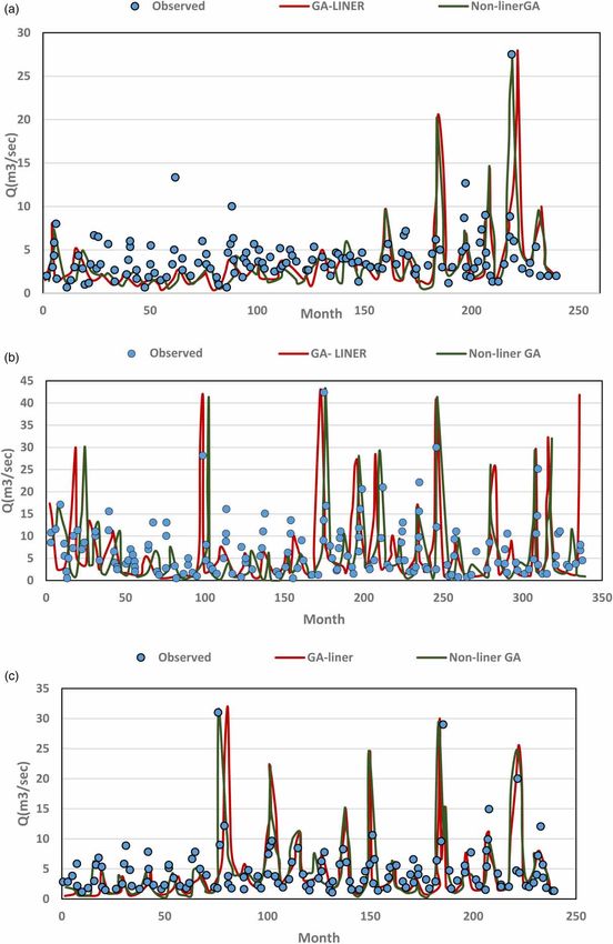
Three comparisons were made in this study. The first one was between the results of the linear GA model with the non-
linear GA model. Table 4 presents the results of the nonlinear GA model with less RMSE and less MAE and more R2 and
NSE between the observed. The predicted amounts were better than the results of the linear GA model in all three studied
stations. For example, in the Chambian station nonlinearity decreased in RMSE and MAE from 1.264 and 0.33 to 1.186 and
0.27, respectively, and increased in R2 and NSE from 0.319 and 0.65 to 0.44 and 0.80, respectively. Figure 5 confirms this
point as well. In fact, non-linearizing improved the results of the GA model in the three studied stations by 27.5%, 17%,
and 9.5% respectively.
The second comparison was between the results of the nonlinear GA model and ANFIS model. Both linear and nonlinear
GA models showed low performance compared to ANFIS. Therefore, the ANFIS model is introduced as a reliable model in
the estimation of runoff. For example, as Table 5 shows for the Dashtbal station, RMSE and MAE from ANFIS results were
Downloaded from http://iwaponline.com/ws/article-pdf/22/10/7460/1127079/ws022107460.pdf
by guestWater Supply Vol 22 No 10, 7468
Figure 3 | Observed and simulated values of runoff. (a) Chambian station (Cham4). (b) Dashtbal station (Dash6). (c) Tangbelaghi (Tang4).
0.054 and 0.17, respectively which were less than RMSE and MAE from nonlinear GA results which were 0.89 and 0.18,
respectively. Also, in the same Dashtbal station R2 and NSE were 0.9 and 0.85, respectively from ANFIS results which
were more than 0.76 and 0.79, respectively from nonlinear GA results.
Downloaded from http://iwaponline.com/ws/article-pdf/22/10/7460/1127079/ws022107460.pdf
by guestWater Supply Vol 22 No 10, 7469
Figure 4 | Correlation between observed and predicted runoff values. (a) Chambian station (Cham 4). (b) Dashtbal station (Dash6).
(c) Tangbelaghi (Tang4).
Table 3 | Relationships resulting from linear and nonlinear modeling of GA
Station Nonlinear model
0:58 0:44
Chambian Runoff ¼ 1:16 þ 0:087P0:85 0:14E0:53 þ 3:53tmean þ 1:15tmax þ 0:77tmin
0:74
Dashtbal Runoff ¼ 0:36 þ 0:42P0:69 0:04E0:35 0:095tmean
1:41
þ 0:11t0:064
max þ 0:77tmin
0:76
Tangbelaghi Runoff ¼ 0:052 þ 0:62P0:46 0:53E0:066 þ 0:12t0:024
mean þ 0:98tmax þ 0:24tmin
0:12 0:35
Linear model
Chambian Runoff ¼ 0:93 þ 0:048P 0:028E 0:079tmean þ 0:155tmax þ 0:315tmin
Dashtbal Runoff ¼ 1:61 þ 0:084P 0:053E 0:67tmean 0:019tmax 0:098tmin
Tangbelaghi Runoff ¼ 1:82 þ 0:03P 0:002E þ 0:176tmean 0:036tmax 0:176tmin
Table 4 | Results from linear and nonlinear models
Linear model Nonlinear model
2
Station R RMSE NSE MAE R2 RMSE NSE MAE
Chambian 0.319 1.264 0.65 0.33 0.44 1.186 0.80 0.27
Dashtbal 0.63 1.024 0.74 0.21 0.76 0.89 0.79 0.18
Tang belaghi 0.57 1.83 0.58 0.32 0.63 1.271 0.72 0.22
Downloaded from http://iwaponline.com/ws/article-pdf/22/10/7460/1127079/ws022107460.pdf
by guestWater Supply Vol 22 No 10, 7470
Figure 5 | Observed runoff (Robs) and predicted runoff (Rsim) versus different months of the studied period. (a) Chambian station. (b) Dashtbal
station. (c) Tangbelaghi station.
Downloaded from http://iwaponline.com/ws/article-pdf/22/10/7460/1127079/ws022107460.pdf
by guestWater Supply Vol 22 No 10, 7471
Table 5 | Results from nonlinear modeling of GA and the best results of ANFIS
Nonlinear model ANFIS
Station R2 RMSE NSE MAE R2 RMSE NSE MAE
Chambian 0.44 1.86 0.8 0.27 0.97 0.08 0.85 0.21
Dashtbal 0.76 0.89 0.79 0.18 0.9 0.054 0.85 0.17
Tang belaghi 0.63 1.271 0.72 0.22 0.98 0.14 0.75 0.24
The third comparison was comparing the ANFIS results with each other by increasing the number of membership func-
tions and running cycles of the model, and using linear membership functions instead of constant membership functions.
Considering Table 2 and Figures 3 and 4 increasing the number of input membership functions and using the linear
output membership function instead of a constant one significantly improves the results of the models. However, the use
of a large number of membership functions (more than 4) makes the calculation process longer, which is not desired in
the simulation and modeling of hydrological phenomena. In fact, as the number of cycles increased, the computation time
increased by approximately 25%. The number of membership functions 3, 4, 5 and 6 were examined for Dashtbal station
in both linear and constant models. As can be seen in Table 2, when the number of membership functions was increased
to four, the amount of model error decreased significantly. However, increasing the number of membership functions to
more than four does not decease error amount considerably but increases the computational time. Therefore, there is no
need to do that, and the two other stations with four membership functions were surveyed. It was clear that using ANFIS,
an increase in the number of membership functions and running cycles of the model decreased the error in Dashtbal, Cham-
bian and Tang Belaghi stations by up to 42, 44 and 11%, respectively.
Meanwhile, as Table 5 shows ANFIS results with less RMSE and less MAE between the observed and the predicted
amounts were better than nonlinear GA results.
Table 5 displays a comparison of the results from the best ANFIS model with GA model in the three stations. The numerical
results indicate that ANFIS with four membership functions and five run rounds worked well in the runoff estimation in the
three stations, e.g. or example for Chambian station these amounts were obtained: RMSE ¼ 0.08, R2 ¼ 0.97, NSE ¼ 0.85 and
MAE ¼ 0.21.While, all these criteria are less accurate in the nonlinear GA model.
Table 6 defines four scenarios, the first of which includes all input parameters to the models. In the second, third and fourth
scenarios rainfall, evaporation, and both parameters (rainfall and evaporation) are removed respectively, to analyze the sen-
sitivity of the models to those parameters.
In Table 7, the sensitivity analysis of ANFIS and nonlinear GA models at the three stations was performed considering
scenarios 1–4.
As can be seen in the table, by removing the main parameter (rainfall), the amounts of error of the models increased for all
three stations. However, the models were not so sensitive when removing evaporation especially using the ANFIS model.
Therefore, runoff can be estimated by using ANFIS in a basin that lacks evaporation data. However, when removing both
parameters of rainfall and evaporation, the error value of the models increased, although ANFIS showed less sensitivity to
reducing the number of input parameters. Meanwhile, the largest difference was observed in the amount of RMSE.
Finally, a summary of the important input and output parameters is given in Table 8. The resulting values in the table also
indicate the accuracy of ANFIS model and the nonlinear model of GA is the second priority.
Table 6 | Scenarios
Scenario Input parameters
Scenario 1 Rainfall–Minimum temperature–Maximum temperature–Average temperature–Evaporation
Scenario 2 Minimum temperature–Maximum temperature–Average temperature–Evaporation
Scenario 3 Rainfall–Minimum temperature–Maximum temperature–Average temperature
Scenario 4 Minimum temperature–Maximum temperature–Average temperature
Downloaded from http://iwaponline.com/ws/article-pdf/22/10/7460/1127079/ws022107460.pdf
by guestWater Supply Vol 22 No 10, 7472
Table 7 | Sensitivity analysis of models
Nonliner-GA ANFIS
Station Input parameters RMSE MAE NSE R2 RMSE MAE NSE R2
Chambian Scenario 1 1.186 0.27 0.8 0.44 0.08 0.21 0.85 0.97
Scenario 2 2.65 0.35 0.67 0.37 0.09 0.23 0.8 0.95
Scenario 3 1.187 0.28 0.77 0.43 0.08 0.21 0.82 0.96
Scenario 4 3.45 0.45 0.56 0.33 0.15 0.33 0.68 0.9
Scenario difference (1 and 2) 1.464 0.08 0.13 0.07 0.01 0.02 0.05 0.02
Scenario difference (1 and 3) 0.001 0.01 0.03 0.01 0 0 0.03 0.01
Scenario difference (1 and 4) 2.264 0.18 0.24 0.11 0.07 0.12 0.17 0.07
Dashtbal Scenario 1 0.86 0.18 0.79 0.76 0.054 0.17 0.85 0.9
Scenario 2 1.03 0.21 0.73 0.7 0.057 0.19 0.8 0.87
Scenario 3 0.87 0.19 0.78 0.74 0.055 0.17 0.83 0.88
Scenario 4 2.56 0.28 0.65 0.6 0.07 0.27 0.74 0.76
Scenario difference (1 and 2) 0.17 0.03 0.06 0.06 0.003 0.02 0.05 0.03
Scenario difference (1 and 3) 0.01 0.01 0.01 0.02 0.001 0 0.02 0.02
Scenario difference (1 and 4) 1.7 0.1 0.14 0.16 0.016 0.1 0.11 0.14
Tangbelaghi Scenario 1 1.271 0.22 0.72 0.63 0.14 0.24 0.75 0.98
Scenario 2 1.56 0.28 0.66 0.58 0.16 0.26 0.7 0.97
Scenario 3 1.269 0.24 0.7 0.61 0.145 0.235 0.74 0.97
Scenario 4 3.32 0.46 0.53 0.44 0.19 0.3 0.65 0.91
Scenario difference (1 and 2) 0.289 0.06 0.06 0.05 0.02 0.02 0.05 0.01
Scenario difference (1 and 3) 0.002 0.02 0.02 0.02 0.005 0.005 0.01 0.01
Scenario difference (1 and 4) 2.049 0.24 0.19 0.19 0.05 0.06 0.1 0.07
Table 8 | Summary of significant parameters
Statistical P Tmin Tmax Tave E QObs Q (ANFIS) Q (Liner-GA) Q (Non-liner-GA)
Station parameter (mm) (C°) (C°) (C°) (mm) (m3/s) (m3/s) (m3/s) (m3/s)
Chambian Average 22.9 11.5 26.3 18.9 196.7 2.94 3.20 4.80 4.72
Minimum 0 3 26.9 5.1 11.5 0 0.25 0.37 0.48
Maximum 243.5 26.9 41 33 592 27.51 27.57 28.10 27.41
Dashtbal Average 32.13 7.7 23.1 15.6 214.5 4.7 6.57 9.56 8.57
Minimum 0 8.6 3.3 1 35.7 0 0.16 0.49 0.23
Maximum 333 22.1 40.5 29.9 549.5 42.4 42.30 43.03 42.58
Tangbelaghi Average 50 5.5 23.1 14.3 151 3.7 4.41 6.07 5.64
Minimum 0 6.2 6.2 0 2.5 0.33 0.37 0.50 0.39
Maximum 441.5 17.2 36.6 26.8 468 31 31.07 32.00 31.28
CONCLUSIONS
Some researchers believe in the use of a large number of independent physiographic and climatic variables (Tavakkoli &
Rostaminia 2006; Salavati et al. 2010). However, since the estimation of runoff in most basins is faced with problems of com-
plexity and lack of data, in this research an attempt was made to provide a simple and practical solution. The neural model
proposed in this study was based on only five climatic parameters which are relatively easy to measure, and at the same time
the results are sufficiently accurate. ANFIS and GA models were employed to estimate runoff using the easily available data
to investigate the rainfall–runoff relationship in three selected hydrometric stations in the Sivand River basin in central Iran.
The amounts of runoff in the selected stations were estimated using easily available climatic data and were compared to the
Downloaded from http://iwaponline.com/ws/article-pdf/22/10/7460/1127079/ws022107460.pdf
by guestWater Supply Vol 22 No 10, 7473
observed runoff values and the comparison result was satisfactory. The input parameters included the average monthly rain-
fall, the monthly minimum, maximum and average temperatures, and the monthly evaporation. Considering the results of the
present study some points should be mentioned are as below.
As the number of membership functions increases, the results of the neuro-fuzzy systems improves, which is consistent with
the results of Ghose et al. (2013) and Hashim et al. (2016). However, when the number of input membership functions is
greater than 4, the computational volume increases and the computational speed decreases. Meanwhile, using ANFIS, the
results from employing the linear output membership function were more accurate than those from employing the constant
output membership function. Moreover, using GA, the nonlinear model was more accurate than the linear one which, could
be attributed to the nonlinear changes of the input parameters.
In general, the results of runoff modeling in the three selected stations using ANFIS were more accurate than the results of
runoff modeling using GA, a conclusion that is in line with the results of Cheng et al. (2005). This result contradicts Asadi’s
result (Asadi et al. 2013) in the runoff prediction that used the hybrid genetic algorithm, and concluded that the hybrid model
of GA was more accurate than ANFIS.
The sensitivity analysis by Hashim et al. (2016) showed that the wet day frequency was the most influential input par-
ameter. Also, Nabizadeh et al. (2012) concluded that temperature has different effects on the predicted amount of runoff
in each month and introduced temperature as an influential parameter. The sensitivity of the results to the input parameters
was investigated in this study too. According to the results removing the rainfall parameter increased the error amount to a
greater extent compared to removing the evaporation parameter, i.e. the models are more sensitive to rainfall than evapor-
ation. In fact, ignoring the evaporation from input data did not have a significant effect on the models’ output, especially
with the ANFIS model. In contrast, ignoring both parameters of rainfall and evaporation from the input data increased
the error amount. Of course, ANFIS showed less error amounts in all three stations.
Since the neuro-fuzzy system is less sensitive to the inaccuracy of the input data, using it is preferred compared to GA. As a
pattern suggested for the optimal ANFIS model for analyzing rainfall–runoff in future, the amount of runoff can be estimated
by entering precipitation data, minimum, maximum, and average temperatures, and evaporation. By analyzing the results
obtained from ANFIS it was observed that the input parameters were satisfactorily enough to estimate runoff in the studied
basin. Due to the proper performance of ANFIS in estimating runoff with climatic data, its results can be trusted and used in
similar projects as well. Meanwhile, based on the results the nonlinear GA model provided better results than the linear one.
Also, the ANFIS model worked more accurately compared to the linear and nonlinear models of GA, so it is recommended as
a simple, applicable, and accurate enough method for calculating runoff using easily available climatic data.
RECOMMENDATION
In this study, due to some limitations, sensitivity analysis was performed on only some of the parameters but not all of them. It
is suggested to perform a sensitivity analysis on the other parameters as well. Also, the role of variance in comparing ANFIS
and PSO-ANFIS models is recommended to be considered. In addition, meteorological parameters such as evapotranspira-
tion, maximum and minimum precipitation, and characteristics of the soil existed in the basin were not available due to the
lack of meteorological data in the Sivand River basin, which could have provided better results if were available.
ACKNOWLEDGEMENT
The authors would like to thank ‘Water Resources Organization’ of Fars province in central Iran for providing the required
data.
DATA AVAILABILITY STATEMENT
All relevant data are included in the paper or its Supplementary Information.
CONFLICT OF INTEREST
The authors declare there is no conflict.
Downloaded from http://iwaponline.com/ws/article-pdf/22/10/7460/1127079/ws022107460.pdf
by guestWater Supply Vol 22 No 10, 7474
REFERENCES
Anusree, K. & Varghese, K. O. 2016 Streamflow prediction of Karuvannur River Basin using ANFIS, ANN and MNLR models. Procedia
Technology 24, 101–108.
Asadi, S., Shahrabi, J., Abbaszadeh, P. & Tabanmehr, S. 2013 A new hybrid artificial neural network for rainfall–runoff process modeling.
Neurocomputing 121, 470–480.
Chandwani, V., Vyas, S. K., Agrawal, V. & Sharma, G. 2015 Soft computing approach for rainfall–runoff modelling: a review. Aquatic
Procedia 4, 1054–1061.
Cheng, C. T., Wu, X. Y. & Chau, K. W. 2005 Multiple criteria rainfall–runoff model calibration using a parallel genetic algorithm in a cluster
of computers. Hydrological Sciences Journal 50 (6), 1069–1087.
Dorum, A., Yarar, A., Sevimli, M. F. & Onüçyildiz, M. 2010 Modelling the rainfall–runoff data of susurluk basin. Expert Systems with
Applications 37 (9), 6587–6593.
Ghose, D. K., Panda, S. S. & Swain, P. C. 2013 Prediction and optimization of runoff via ANFIS and GA. Alexandria Engineering Journal
52 (2), 209–220.
Goldberg, D. E. 1989 Genetic Algorithms in Search, Optimization, and Machine Learning. Addison-Wesley Longman Publishing Co, Inc.,
Boston, Ma, USA.
Hashim, R., Roy, C., Motamedi, S., Shamshirband, S., Petković, D., Gocic, M. & Lee, S. C. 2016 Selection of meteorological parameters
affecting rainfall estimation using neuro-fuzzy computing methodology. Atmospheric Research 171 (1), 21–30.
Holland, J. H. 1975 Review of Adaptation in Natural and Artificial Systems. The University of Michigan Press, ACM SIGART Bulletin,
New York, United States, pp. 15–15.
Huang, M., Zhang, T., Ruan, J. & Chen, X. 2017 A new efficient hybrid intelligent model for biodegradation process of DMP with fuzzy
wavelet neural networks. Scientific Reports 7 (1), 1–9.
Jang, J. S. 1993 ANFIS: adaptive-network-based fuzzy inference system. IEEE Transactions on Systems, Man, and Cybernetics 23 (3), 665–685.
Jang, J. S. & Sun, C. T. 1995 Neuro-fuzzy modeling and control. Proceedings of the IEEE 83 (3), 378–406.
Jothiprakash, V., Magar, R. B. & Kalkutki, S. 2009 Rainfall–runoff models using adaptive neuro–fuzzy inference system (ANFIS) for an
intermittent River. International Journal of Artificial Intelligence 3, 1–23.
Kan, G., Liang, K., Yu, H., Sun, B., Ding, L., Li, J., He, X. & Shen, C. 2020 Hybrid machine learning hydrological model for flood forecast
purpose. Open Geosciences 12 (1), 813–820.
Khoshnevisan, B., Rafiee, S., Omid, M. & Mousazadeh, H. 2014 Development of an intelligent system based on ANFIS for predicting wheat
grain yield on the basis of energy inputs. Information Processing in Agriculture 1 (1), 14–22.
Kumanlioglu, A. A. & Fistikoglu, O. 2019 Performance enhancement of a conceptual hydrological model by integrating artificial intelligence.
Journal of Hydrologic Engineering. Available from: https://ascelibrary.org/doi/epdf/10.1061/%28ASCE%29HE.1943-5584.0001850
(accessed 19 August 2019)
Kumar, S., Roshni, T. & Himayoun, D. 2019 A comparison of emotional neural network (ENN) and artificial neural network (ANN)
approach for rainfall–runoff modelling. Civil Engineering Journal 5 (10), 2120–2130.
Liu, Z. 2010 Chaotic time series analysis. Mathematical Problems in Engineering. Available from: https://www.hindawi.com/journals/mpe/
2010/720190/ (accessed 13 Apr 2010).
Marouf, H., Hashemi, M. & Diba, T. 2015 Modeling of rainfall–runoff of Velian river using GA and comparison with experimental
relationships, MSC. Faculty of civil engineering. Maragheh University, p. 123.
Moraga, C. & Salas, R. 2005 A new aspect for the optimization of fuzzy if-then rules. In 35th International Symposium on Multiple-Valued
Logic (ISMVL’05), 19–21 May, Canada.
Morales, Y., Querales, M., Rosas, H., Allende-Cid, H. & Salas, R. 2021 A self-identification neuro-fuzzy inference framework for modeling
rainfall–runoff in a Chilean watershed. Journal of Hydrology 594, 125910–125927.
Nabizadeh, M., Mosaedi, A. & Dehghani, A. A. 2012 Intelligent estimation of stream flow by adaptive neuro-fuzzy inference system. Water
and Irrigation Management 2 (1), 69–80.
Nath, A., Mthethwa, F. & Saha, G. 2020 Runoff estimation using modified adaptive neuro-fuzzy inference system. Environmental Engineering
Research 25 (4), 545–553.
Nauck, D. D. & Nürnberger, A. 2013 Neuro-fuzzy systems: a short historical review. In: Computational Intelligence in Intelligent Data
Analysis, pp. 91–109. Springer, Berlin, Heidelberg.
Panchal, R., Suryanarayana, T. M. V. & Parekh, F. P. 2014 Adaptive neuro-fuzzy inference system for rainfall–runoff modeling. International
Journal of Engineering Research and Applications 4, 202–206.
Roy, B., Singh, M. P. & Singh, A. 2019 A Novel Approach for Rainfall-Runoff Modelling Using A Biogeography-Based Optimization.
Available from: https://www.tandfonline.com/loi/trbm20 (accessed 26 June 2019).
Salavati, B., Sadeghi, S. J. & Telori, A. 2010 Modeling runoff production in watersheds of Kurdistan province using physiographic and
climatic variables. Water and Soil (Agricultural Sciences and Industries) 24 (1), 84–96.
Ş en, Z. & Altunkaynak, A. 2004 Fuzzy awakening in rainfall–runoff modeling. Hydrology Research 35 (1), 31–43.
Suparta, W. & Samah, A. A. 2020 Rainfall prediction by using ANFIS times series technique in South Tangerang, Indonesia. Geodesy and
Geodynamics 11 (6), 411–417.
Downloaded from http://iwaponline.com/ws/article-pdf/22/10/7460/1127079/ws022107460.pdf
by guestWater Supply Vol 22 No 10, 7475
Takagi, T. & Sugeno, M. 1985 Fuzzy identification of systems and its applications to modeling and control. IEEE Trans. on Systems, Man, and
Cybernetics 15 (1), 116–132.
Talei, A., Chua, L. H. C. & Quek, C. 2010 A novel application of a neuro-fuzzy computational technique in event-based rainfall–runoff
modeling. Expert Systems with Applications 37 (12), 7456–7468.
Tavakkoli, M. & Rostaminia, M. 2006 Presenting a regional flood model in the watersheds of Ilam province. Journal of Iranian Agricultural
Sciences 20 (2), 347–356.
Tayebiyan, A., Mohammad, T. A., Malakootian, M., Nasiri, A., Heidari, M. R. & Yazdanpanah, G. 2019 Potential impact of global warming on
river runoff coming to Jor reservoir, Malaysia by integration of LARS-WG with artificial neural networks. Environmental Health
Engineering and Management Journal 6 (2), 139–149.
Zahedi, F. & Zahedi, Z. 2018 A review of neuro-fuzzy systems based on intelligent control. Journal of Electrical and Electronic Engineering
3 (2/1), 58–61.
Zhihua, L. V., Zuo, J. & Rodriguez, D. 2020 Predicting of runoff using an optimized SWAT-ANN: a case study. Journal of Hydrology: Regional
Studies 29, 100688. https://doi.org/10.1016/j.ejrh.2020.100688.
First received 20 April 2022; accepted in revised form 25 August 2022. Available online 2 September 2022
Downloaded from http://iwaponline.com/ws/article-pdf/22/10/7460/1127079/ws022107460.pdf
by guestYou can also read