Rosalia: an experimental research site to study hydrological processes in a forest catchment
←
→
Page content transcription
If your browser does not render page correctly, please read the page content below
Earth Syst. Sci. Data, 13, 4019–4034, 2021
https://doi.org/10.5194/essd-13-4019-2021
© Author(s) 2021. This work is distributed under
the Creative Commons Attribution 4.0 License.

                 Rosalia: an experimental research site to study
                  hydrological processes in a forest catchment
            Josef Fürst1 , Hans Peter Nachtnebel1 , Josef Gasch2 , Reinhard Nolz3 , Michael Paul Stockinger3 ,
                                        Christine Stumpp3 , and Karsten Schulz1
                   1 Institute
                             for Hydrology and Water Management (HyWa), University of Natural Resources
                                        and Life Sciences Vienna (BOKU), Vienna, Austria
                                  2 Forest Demonstration Centre, University of Natural Resources

                                        and Life Sciences Vienna (BOKU), Vienna, Austria
             3 Institute for Soil Physics and Rural Water Management (SoPhy), University of Natural Resources

                                        and Life Sciences Vienna (BOKU), Vienna, Austria
                                        Correspondence: Josef Fürst (josef.fuerst@boku.ac.at)

                                      Received: 27 August 2020 – Discussion started: 26 November 2020
                                 Revised: 29 June 2021 – Accepted: 14 July 2021 – Published: 19 August 2021

       Abstract. Experimental watersheds have a long tradition as research sites in hydrology and have been used
       since the late nineteenth and early twentieth centuries. The University of Natural Resources and Life Sciences
       Vienna (BOKU) recently extended its experimental research forest site “Rosalia” with an area of 950 ha towards
       the creation of a full ecological-hydrological experimental watershed. The overall objective is to implement a
       multi-scale, multi-disciplinary observation system that facilitates the study of water, energy and solute transport
       processes in the soil–plant–atmosphere continuum. This article describes the characteristics of the site and the
       monitoring network and its instrumentation that has been installed since 2015, as well as the datasets. The net-
       work includes four discharge gauging stations and seven rain gauges along with observations of air and water
       temperature, relative humidity, and electrical conductivity. In four profiles, soil water content and temperature
       are recorded at different depths. In addition, since 2018, nitrate, TOC and turbidity have been monitored at
       one gauging station. In 2019, a programme to collect isotopic data in precipitation and discharge was initiated.
       All data collected since 2015, including, in total, 56 high-resolution time series (with 10 min sampling inter-
       vals), are provided to the scientific community on a publicly accessible repository. The datasets are available at
       https://doi.org/10.5281/zenodo.3997140 (Fürst et al., 2020).

1   Introduction                                                        Given these long-term datasets, changes in the hydrological
                                                                        cycle, such as those resulting from climate warming, can be
                                                                        investigated in these watersheds (Bogena et al., 2018).
Environmentally oriented water management depends on un-                   In recent decades, there has been growing recognition that
derstanding hydrological processes and their dominant con-              hydrology (and its related disciplines) cannot be treated in
trols at different spatial and temporal scales. To investi-             isolation. Rather, hydrological processes driven by meteoro-
gate hydrological processes and their complex interactions              logical conditions are also strongly controlled by complex
with the environment, long-term measurements from multi-                feedback mechanisms with biotic and abiotic systems (Por-
disciplinary hydrological observatories are required (Schu-             porato and Rodriguez-Iturbe, 2002). Therefore, hydrologi-
mann et al., 2010; Blöschl et al., 2016). As the earliest hy-           cal experimental watersheds have gradually transitioned into
drological observatories, experimental watersheds have been             multi-disciplinary experimental watersheds. A prominent ex-
used as far back as the late nineteenth and early twenti-               ample for this is the “Critical Zone Observatories” research
eth centuries (USGS Reynolds Creek; Seyfried et al., 2018).

Published by Copernicus Publications.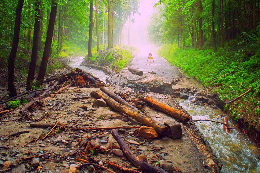
4020                                                                                                      J. Fürst et al.: Rosalia

project, which was initiated in 2007 by the US National Sci-      subsurface. The Plynlimon research catchment in the UK
ence Foundation (Anderson et al., 2018) and has been suc-         (Neal et al., 2011; Cosby and Emmett, 2020) and the Kryck-
ceeded by the Critical Zone Collaborative Network (CZN) in        lan catchment study in Sweden (Laudon et al., 2013) are
2021.                                                             good examples of such research catchments, with long term
   Understanding processes based on research conducted at         tracer and hydro-geochemical data available.
individual catchments is limited to the physio-geographic            The University of Natural Resources and Life Sciences
conditions at the particular location. In an effort to un-        in Vienna (BOKU) has a long tradition and extensive ex-
derstand hydrological processes based on a wider spec-            perience in operating multi-disciplinary experimental sites.
trum of boundary conditions, networks of multi-disciplinary       BOKU has been using these sites for research purposes to
hydrological observatories have been established in recent        monitor environmental changes and climate change impacts,
decades. Examples of such networks are the German “TER-           to develop new monitoring techniques, and to train students
restrial ENvironmental Observatory network” (TERENO)              in applied research. One of BOKU’s sites is the experimental
(Zacharias et al., 2011), the “International Network for          research forest “Rosalia”, with an area of 950 ha that was es-
Alpine Research Catchment Hydrology” (Bernhardt et al.,           tablished in 1875 to facilitate research and education, mainly
2015), the “US National Science Foundation’s National Eco-        in forestry disciplines (Fig. 1). Several forest dieback stud-
logical Observatory Network” (NEON) (Kampe et al., 2010),         ies were conducted in the 1980s. In 2013, a 222 ha water-
and the “Euro-Mediterranean Network of Experimental and           shed within the Rosalia forest site was established as an eco-
Representative Basins” (ERB) as part of UNESCO FRIEND             hydrological experimental watershed, and this Rosalia wa-
(Flow Regimes from International Experimental and Net-            tershed became part of the Austrian LTER-CWN (Research
work Data) (Holzmann, 2018).                                      Infrastructure for Carbon, Water and Nitrogen) initiative.
   A prominent example of an observatory network is the              The overall objective is to implement a multi-scale, multi-
“Long-Term Ecosystem Research” (LTER) initiative, which           disciplinary observatory that facilitates the study of wa-
aims to better understand the structure and functioning of        ter, energy and solute transport processes in the soil–plant–
complex ecosystems and their long-term response to environ-       atmosphere continuum. Research emphasis is put on deriv-
mental, societal and economic pressures at different spatial      ing effective parameters for scales on which models simu-
scales (LTER Network Office, 2020). The LTER was initi-           late flow and transport processes (e.g. hillslope, catchment)
ated in 1980 with six US catchments and has since expanded        by upscaling point measurements. A distinctive feature of
to other continents, comprising different ecosystem types,        the current monitoring setup is the continuous measurement
climates and pressures. The LTER was further developed into       of tracers in precipitation and discharge of selected creeks
the “Long Term Socio-economic and Ecosystem Research”             within the catchment, which allows us to derive travel time
(LTSER) platform to emphasise the importance of the hu-           distributions for sub-catchments and investigate flow path-
man dimension and to explicitly consider the socio-economic       ways in detail. Because BOKU has the right of access for
system in multi-disciplinary ecosystem research (Haberl et        educational and research purposes, large-scale controlled ex-
al., 2006). The European LTER is the “European Long-Term          periments can be undertaken. For example, rain-out shelters
Ecosystem, Critical Zone and Socio-Ecological Systems Re-         were used in parts of the forest by Netherer et al. (2015) to in-
search Infrastructure” (eLTER RI), which was established in       vestigate drought impacts on bark beetle attacks on Norway
2003 by the European Commission as part of the “European          spruce, while Schwen et al. (2015) and Leitner et al. (2017)
Strategy Forum on Research Infrastructures” (ESFRI) (ES-          used rain-out shelters to investigate soil water repellency and
FRI, 2020).                                                       short-term organic nitrogen fluxes under a changing climate.
   These networks of observatories make it possible to ad-        Besides such local experiments, the monitoring network es-
dress some open research questions in hydrology that were         tablished in 2015 enables researchers to investigate the im-
recently formulated (Blöschl et al., 2019). The most chal-        pacts on the large-scale forest ecosystem and its services
lenging questions regarding catchment hydrology relate to         by providing the necessary baseline data. Investigating the
the effect of small-scale variability in the upscaling of model   transition of the forest ecosystem from its actual state into a
parameters and processes (e.g., hydraulic conductivity and        pristine, unmanaged natural forest is among future research
porosity of soils, soil water movement), the transfer of model    plans.
parameters to other (especially ungauged) catchments, and            The objective of this article is to present the monitoring
the derivation of flow paths and residence times of water         network and the recorded data of the Rosalia watershed and
and solutes in the subsurface at different scales. Overcoming     to make them available to the scientific community.
these challenges requires the existing networks of observa-
tories to be complemented in their instrumentation and ob-
servational capacities, harmonising temporal and spatial fre-     2   Description of the watershed
quencies and continuously monitoring natural tracers such
as ions, metals and stable isotope ratios such as 2 H/1 H,        The Rosalia watershed is part of the Rosalia mountains (Ger-
18 O/16 O and 15 N/14 N in precipitation, discharge and the       man: Rosaliengebirge) that belong to the eastern foothills

Earth Syst. Sci. Data, 13, 4019–4034, 2021                                        https://doi.org/10.5194/essd-13-4019-2021
J. Fürst et al.: Rosalia                                                                                                     4021

Figure 1. Map of the watersheds and the monitoring network (DEM source: Land Niederösterreich – http://data.noe.gv.at, last access:
29 June 2021).

of the Alps on the state border between Lower Austria
and Burgenland in Austria (Fig. 1). Terrain heights range
from 385 to 725 m a.s.l., and the watershed is characterised
by steep slopes (96 % of the area is steeper than 10 %,
and 55 % is steeper than 30 %). From 1990 to 2017, an-
nual precipitation was between 560 and 1100 mm (aver-
age 790 mm, standard deviation 128 mm), and the mean an-
nual air temperature was between 5.5 and 10 ◦ C (average
8.2 ◦ C, standard deviation 1.2 ◦ C) (data: https://deims.org/
dataset/839e7779-f6ee-4b81-b4d8-924177b9c562, last ac-
cess: 29 June 2021). Precipitation is not equally distributed
throughout the year. Frequently in summer, heavy thunder-
storms occur, causing floods that destroy forest roads, road
culverts and other infrastructure (Fig. 2).
   Crystalline rocks dominate in the Rosalia mountains, but         Figure 2. Destructions of forest roads due to a storm on
coarse-grained gneiss, sericitic schist, phyllite and dolomite      29 June 2009 (Photo: Josef Gasch).
are also encountered. However, only coarse-grained gneiss
with occasionally embedded dark or white mica schist is
found in the actual catchment area of the hydrological re-
search site.                                                        are characterised by poor water holding capacity and loss
   The soils are predominantly cambisols that can be clas-          of organic material due to gravitational transport and wind
sified into four categories (Fig. 3). The source materials for      erosion. The characteristic species for these sites are beech
the recent soil formation are often remnants of tertiary soils      with white woodrush (Luzula albida) associated with pine
that were modified by frost action and landslides during the        (Pinus sylvestris) and European larch (Larix decidua) above
ice age. The cambisols on steep slopes (slope > 40 %, cate-         500 m a.s.l., while below 500 m a.s.l. they are associated with
gory 1 in Fig. 3) cover 5 % of the area. They are podzolic          oak (Quercus petraea). Cambisols on plains and moderate
cambisols with more than 40 % coarse grain. These sites             slopes (category 2 in Fig. 3, 68 % of the area) contain 30 %–
                                                                    50 % coarse grain and have a medium water holding capac-

https://doi.org/10.5194/essd-13-4019-2021                                          Earth Syst. Sci. Data, 13, 4019–4034, 2021
4022                                                                                                        J. Fürst et al.: Rosalia

                                                                   snow break, wind throw and bark beetles, the latter affecting
                                                                   mainly coniferous tree species.
                                                                      The main advantages of Rosalia as a research site are as
                                                                   follows:

                                                                       1. The watershed is part of the larger 950 ha forest site
                                                                          used by BOKU, and therefore a large amount of wa-
                                                                          tershed information already exists, including soil maps,
                                                                          high-resolution DEMs (digital elevation models), maps
                                                                          on forest growth and productivity, detailed topographic
                                                                          maps, etc.

                                                                       2. There is a well-established cooperation between BOKU
                                                                          and the owners of the forest, the Austrian Federal
                                                                          Forests, which facilitates even large-scale experiments
                                                                          with durations of several years.

                                                                       3. Rosalia can be reached from Vienna within less than an
Figure 3. Soil map with the four main soil categories, watershed
                                                                          hour, making maintenance cost-effective.
divides and discharge gauges.
                                                                       4. BOKU has an educational centre right at the border of
                                                                          the watershed with seminar rooms, basic laboratory fa-
ity. The characteristic species is beech with woodruff (Gal-              cilities and accommodation for up to 40 persons. Resi-
ium odoratum). At higher elevations and cool north slopes,                dent staff at the educational centre can assist in urgent
beech, spruce and fir (abieti-fagetum) are found. Cambisol                situations, such as a storm or power failure.
and planosol on plains and moderate slopes (category 3 in
Fig. 3, 22 % of the area) are characterised by periodic wa-        3     Network of measurement sites
ter stagnation. They are typically on concave land forms and
have good water capacity and nutrient sustenance. There is         A network of stations (Fig. 1, Tables 1 and 2) has been set
a risk of wind throw due to possible root dieback in long          up to collect hydro-meteorological data: at four gauging sta-
wet periods. Forest associations are the same as for category      tions, river discharge, water and air temperature, relative hu-
2. Cambisol and fluvisol on valley slopes and bottoms (cat-        midity, and electrical conductivity of water are monitored.
egory 4, 5 % of the area) are characterised by varying con-        The locations were selected to cover nested sub-watersheds
tents of coarse material and profile thickness but always have     of 9, 27, 146 and 222 ha. At one of these sites (Q4, 146 ha),
good nutrient and water supply. Where valleys form a flat          water quality (NO3 -N, TOC, turbidity) is monitored with a
bottom, fluvisols are the basis for plant growth. The domi-        S::can multi::lyser™ spectrometer probe. Here, also stream
nant tree species on the slopes are ash and sycamore (aceri-       water samples are taken for analysing stable isotopes of oxy-
fraxinetum), while ash and black alder (pruno-fraxinetum)          gen (δ 18 O) and hydrogen (δ 2 H). Precipitation is measured
dominate the valley floors.                                        by seven rain gauges at different altitudes. At two of these
   Forest management is undertaken by the Austrian Federal         locations, K1 and Q4, precipitation is additionally collected
Forests (OeBf; Österreichische Bundesforste) owned by the          for the analysis of δ 18 O and δ 2 H. At four locations, soil pro-
Republic of Austria. BOKU has the right of access for ed-          files were equipped with sensors measuring soil water con-
ucational and research purposes. OeBf manages the forest           tent (SWC), electrical conductivity of soil water, and soil
sustainably, balancing the protection of the environment, the      temperature at four and three depths, respectively.
needs of society and economic success. The management of
the forest is characterised by long production cycles of 100 to
                                                                   3.1    Data acquisition
140 years. The main species of the forest are the broadleaved
beech (Fagus sylvatica) and the coniferous Norway spruce           Although the observed variables have different temporal
(Picea abies). The forest is at different development stages       characteristics, it was decided to record all in situ mea-
ranging from clear cut areas to mature forest stands. Natu-        surements (except stable water isotope data) at synchronous
ral regeneration is preferred to planting, and fertilisation is    10 min intervals to simplify data storage and organisation.
almost never done. Timber harvesting is usually done with          For this purpose, a UHF radio telemetry network (ADCON
harvesters and forwarders, and cable cranes are used on steep      telemetry by OTT Hydromet GmbH) was implemented, en-
slopes. Management and timber transport are supported by           abling data acquisition, storage and management by a web-
a dense network of forest roads (50 m per hectare), suit-          accessible database management system (DBMS). At each
able for heavy timber trucks. Main threats to the forest are       monitoring site, different sensors are connected to a remote

Earth Syst. Sci. Data, 13, 4019–4034, 2021                                           https://doi.org/10.5194/essd-13-4019-2021
J. Fürst et al.: Rosalia                                                                                                                     4023

Table 1. List of sites, sensors and observed variables.

      Site                     Sensors                                                       Observed variables
                               Conductivity and temperature sensor Ponsel C4E                Electrical conductivity and water temperature
      Q1
      Mittereckgraben          Rain gauge RG1 (Adcon tipping bucket)                         10 min rain depth
      559.87 m a.s.l
                               Air temperature and humidity sensor TR1 (Adcon)               Air temperature
      Watershed 9 ha
                                                                                             Relative humidity
                               1-ft H-flume with two ultrasonic distance sensors (Baumer)    Water level in H-flume
                                                                                             Discharge
                               Tipping bucket, 1 L per tip (for discharge < 0.02 L s−1 )     Small discharge
      Q1S0                     Four HydraProbe soil sensors (Stevens) at Q1S0                Soil water content
      Soil water profile       Sensor depths: 10, 20, 40, 60 cm                              Soil temperature
                                                                                             Electrical conductivity of soil water
      Q2                       Conductivity and temperature sensor Ponsel C4E                Electrical conductivity
      Grasriegelgraben                                                                       Water temperature
      550.06 m a.s.l
                               Rain gauge RG1 (tipping bucket)                               10 min rain depth
      Watershed 27 ha
                               Air temperature and humidity sensor TR1                       Air temperature
                                                                                             Relative humidity
                               1-ft H-flume with two ultrasonic distance sensors             Water level in H-flume
                                                                                             Discharge
      Q2S0                     Four HydraProbe soil sensors at Q2S0                          For parameters, see above
      Soil water profile       Sensor depths: 10, 20, 40, 60 cm
      Q2S1                     Three HydraProbe soil sensors at Q2S1 and Q2S2                For parameters, see above
      Q2S2                     Sensor depths: 10, 20, 40 cm
      Soil water profiles
      Q3                       Depth sensor Keller PR46X                                     Water level at weir
      Weir Grasriegelgraben                                                                  Discharge
      410 m a.s.l
                               Rain gauge RG1 (tipping bucket)                               10 min rain depth
      Watershed 222 ha
                               Air temperature and humidity sensor TR1                       Air temperature
                                                                                             Relative humidity
                               2-ft H-flume with two ultrasonic distance sensors (Baumer)    Water level in H-flume
                                                                                             Discharge
      Q4
      Grasriegelgraben         Rain gauge RG1 (tipping bucket)                               10 min rain depth
      415 m a.s.l
                               Air temperature and humidity sensor TR1                       Air temperature
      Watershed 146 ha
                                                                                             Relative humidity
                               S::can conductivity and temperature sensor condu:lyser        Electrical conductivity
                                                                                             Water temperature
                               S::can multi::lyser spectrometer probe                        TOC, NO3 -N, turbidity
                               Palmex rain sampler                                           Precipitation isotopes (δ 18 O, δ 2 H)
                               Teledyne ISCO full-size portable sampler 6712                 River water isotopes (δ 18 O, δ 2 H)
      K1                       OTT Pluvio2 L – weighing rain gauge                           10 min rain depth
      Heuberg
                               Air temperature and humidity sensor TR1                       Air temperature
      640 m a.s.l
                                                                                             Relative humidity
                               Palmex – rain sampler                                         Precipitation isotopes (δ 18 O, δ 2 H)
      K2                       OTT Pluvio2 L – weighing rain gauge                           10 min rain depth
      Mehlbeerleiten
                               Air temperature and humidity sensor TR1                       Air temperature
      385 m a.s.l
                                                                                             Relative humidity
      K3                       OTT Pluvio2 L – weighing rain gauge                           10 min rain depth
      Krieriegel
      655 m a.s.l

https://doi.org/10.5194/essd-13-4019-2021                                                   Earth Syst. Sci. Data, 13, 4019–4034, 2021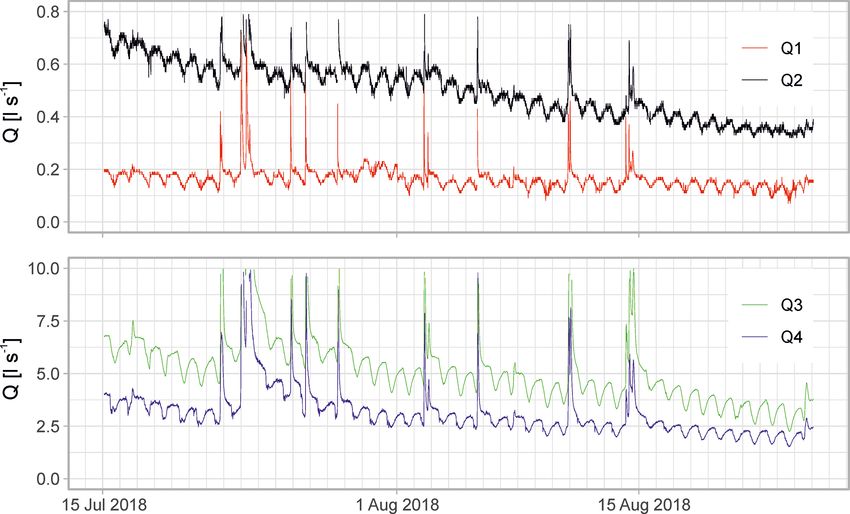
4024                                                                                                           J. Fürst et al.: Rosalia

Table 2. Specifications of sensors. Last access date of all URLs: 29 June 2021.

  Sensor                             Variable                           Range                Resolution       Accuracy
  Adcon RG1 tipping bucket rain      Precipitation (mm)                 0–200 mm/h           0.2 mm           < 50 mm h−1 ± 1 %
  gauge                                                                                                       50–100 mm h−1 ± 3 %
  http://www.adcon.at                                                                                         100–
                                                                                                              200 mm h−1 ± 5 %
  Ott Pluvio2 weighing               Precipitation (mm)                 12–                  0.01 mm min−1    ±0.05 mm
  rain gauge                                                            1800 mm h−1
  https://www.ott.com
  Adcon TR1 air temperature and      Air temperature (◦ C)              −40 to +60 ◦ C       ±0.1 ◦ C         ±0.1 ◦ C
  humidity                           Relative humidity (% RH)           0–100 % RH                            ± 1 % RH at 0 % RH–
  http://www.adcon.at                                                                                         90 % RH
                                                                                                              ±2 % RH at 90 % RH–
                                                                                                              100 % RH
  UGT – 1-ft H-flume                 Discharge (L s−1 )                 0.02–55 L s−1                         2 %–5 %
  https://www.ugt-online.de
  UGT – 2-ft H-flume                 Discharge (L s−1 )                 0.04–315 L s−1                        2 %–5 %
  https://www.ugt-online.de
  Keller PR-46X water level          Water level (m)                    0–1 m                < 1 mm           ±0.55 mm
  https://keller-druck.com
  Ponsel C4E water                   Water temperature (◦ C)            0–50 ◦ C             0.01 ◦ C         ±0.5 ◦ C
  temperature and electrical         Electrical conductivity            0–2000 µS cm−1       < 0.1 µS cm−1    ±1 % of the full range
  conductivity                       (µS cm−1 )
  https://en.aqualabo.fr
  s::can condu::lyser™ water         Water temperature (◦ C)            −20–130 ◦ C          < 0.1 ◦ C        Not specified
  temperature and electrical         Electrical conductivity            0–                   1 µS cm−1        ±1 % of value
  conductivity                       (µS cm−1 )                         500 000 µS cm−1
  https://www.s-can.at
  Stevens HydraProbe II              Soil water content (cm3 cm−3 )     Dry to saturated                      ±3 %
  https://www.stevenswater.com       Electrical conductivity            0–20 dS m−1                           ±2 % or ±0.2 dS m−1
                                     (dS m−1 )
                                     Soil temperature (◦ C)             −10 to +65 ◦ C                        ±0.6 ◦ C

telemetry unit (RTU). Within the network, several RTUs                  of hardware state and broadcasting parameters. Pre-defined
store and transmit data to a base station (located at the educa-        conditions, such as power failure or exceedance of certain
tion centre building) and receive control commands from the             thresholds in the data, can trigger e-mail alerts to site admin-
base station. Apart from physically connecting the sensors to           istrators to enable timely remediation of issues, avoiding or
the RTU and providing a power supply (solar or external),               reducing gaps in the records.
all setup, parameterisation, etc. are done remotely via a web              Stable water isotope data are not automatically uploaded
interface to the base station.                                          to the DBMS, but samples are collected on-site and picked
   The DBMS addVANTAGE Pro, which is connected to                       up manually by university staff for analysis in the labora-
the base station via an internet link, is the main interface            tory. Precipitation samples are collected bi-weekly with to-
for administrators, regular users and the public. It is AD-             talisators with plans to refine the sampling interval to daily,
CON’s universal data visualisation, processing and distribu-            while streamflow samples are collected as daily grab samples
tion platform. It is fully web-based, runs on a reliable Post-          using an autosampler.
greSQL database engine and is fully scalable from a sin-
gle user version for five RTUs to servers with thousands of
clients and thousands of RTUs. The addVANTAGE Pro inter-
face was configured to provide intuitive diagnostic displays
of the measured hydro-meteorological variables, as well as

Earth Syst. Sci. Data, 13, 4019–4034, 2021                                                 https://doi.org/10.5194/essd-13-4019-2021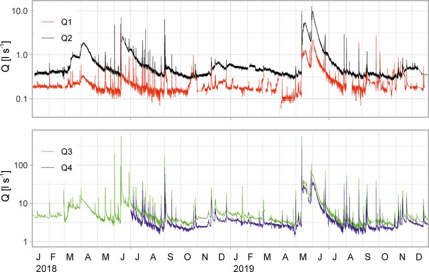
J. Fürst et al.: Rosalia 4025
3.2 Description of sites 3.2.2 Rain gauges
3.2.1 Discharge gauges Sites K1, K2 and K3 are equipped with OTT Pluvio2 weigh-
ing rain gauges. Antifreeze fluid is added during the frost
The sites for discharge measurements were selected to col-
period so that continuous measurements are possible. At the
lect data for nested sub-catchments of different sizes. It was
discharge sites Q1 to Q4, tipping bucket rain gauges are in-
possible to find locations just at culverts of forest access
stalled. They require more maintenance than weighing rain
roads, which has several advantages: (i) the sites are accessi-
gauges because the funnel is easily blocked by deposition of
ble by car, which is important for cost-effective maintenance;
leaves, pollen, dust or insects, and they are inoperable dur-
(ii) they have a defined sub-catchment outlet; and (iii) the H
ing frost. Records from November to April must therefore be
flume devices could be mounted directly on culverts, which
carefully checked using air temperature records and compar-
meant that the road embankments could be used to fully cap-
ing the data with the records from the weighing rain gauges.
ture even larger flows.
Furthermore, it was not possible to place all rain gauges in
H-flume devices were selected to measure discharge as
the forest in such a way that no negative wind influences
they cover a wide range of flow rates and most sediments
occur. Particularly, the recommendation that the height of
are flushed through due to their horizontal bottom (Morgen-
nearby objects, such as trees, should not exceed the distance
schweis, 2010). For sites Q1 and Q2 with a watershed size
from the gauge to the objects (WMO, 2008) had to be disre-
of 9 and 27 ha, respectively, the 1-foot H-flumes can mea-
garded for Q1 and Q2. In particular, the rain gauge at Q1 is
sure discharge from 0.02 up to 55 L s−1 , in which the upper
directly affected by the interception of the trees above.
limit corresponds to an approximately 5-year flood discharge
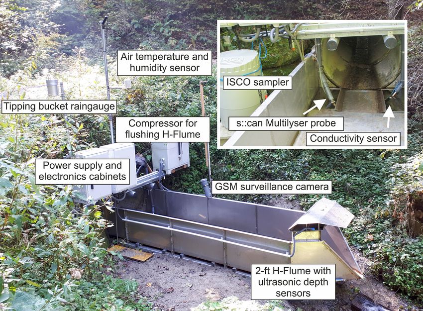
(at the 27 ha site). Site Q4, with a watershed of 146 ha, is
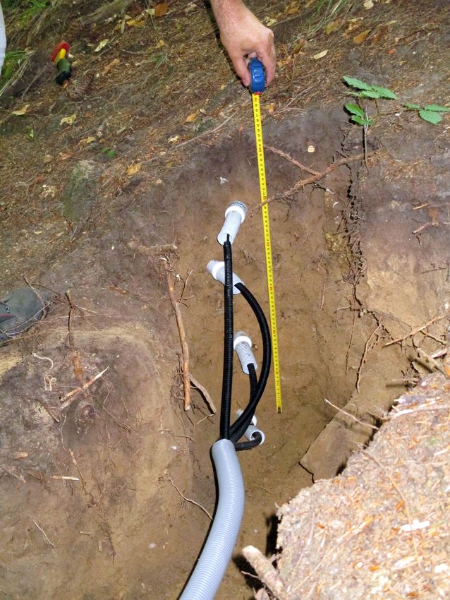
3.2.3 Soil water
equipped with a 2-foot H flume (Fig. 4). Water level at the
H-flumes is measured by pairs of ultrasonic distance sensors. Stevens® HydraProbe® soil sensors (Stevens Water Monitor-
One of these sensors measures the depth to the water level, ing Systems, Inc., Portland, OR, USA) were installed to si-
and the second measures a fixed reference distance. With the multaneously measure soil moisture, temperature and salin-
ratio of known reference distance to measured distance, the ity (Stevens Water Monitoring Systems, 2015). The sensors
depth to water level is corrected for the dependence of the deliver a standard data packet of six variables, including three
speed of sound on air temperature and relative humidity. Al- variables characterising the dielectric properties of the soil
though H-flumes are comparatively insensitive to sediment and the resulting values of soil water content, temperature
accumulation, we developed a compressed-air flushing sys- and bulk electrical conductivity. The sensor-internal calcu-
tem to keep the outflow section and the water level reference lation of soil water content refers to the general calibration
point free of sediments and debris. Site Q3 (222 ha) was al- function published by Seyfried et al. (2005). In total, four
ready constructed in the 1980s using a Thomson weir (Thom- soil profiles were equipped with HydraProbes. In two of the
son, 1859). The water level at Q3 is measured by a capacitive profiles, the sensors were installed at depths of 10, 20, 40
pressure transmitter. and 60 cm below the surface (Fig. 5); in the others, the sen-
Sites Q1, Q2 and Q4 are additionally equipped with sen- sors were installed at 10, 20 and 40 cm depth. Soil profile
sors for electrical conductivity, water temperature, air tem- Q1S0 is located approximately 20 m upslope of gauge Q1.
perature and relative humidity. At sites Q1 and Q2, Ponsel Soil profiles Q2S0, Q2S1 and Q2S2 form a transect up the
C4E sensors (four electrodes) were installed to measure wa- slope line at 16, 30 and 45 m distance from Q2. This design
ter temperature and conductivity as they have an SDI-12 in- supports a transect of soil water parameters measured along
terface and low power consumption. They work electroni- the slope line (Fig. 1).
cally reliably, but the measured conductivities are sensitive
to biofilms on the sensor, and the internal firmware requires 3.2.4 Water quality
more than an hour to achieve a stable reading after turning
on or after cleaning. Furthermore, the measured conductiv- Since 2018, the water quality parameters NO3 -N, TOC and
ity tends to show an offset compared to manual measure- turbidity have been monitored with a spectrometer probe,
ments conducted approximately bi-weekly. Nevertheless, the s::can multi::lyser™, at site Q4. In June 2019, two rain total-
recorded curves show plausible dynamics, e.g., during storm isators (Palmex Ltd., Croatia) specifically designed to min-
events. Currently, alternative sensors are being tested to re- imise isotope fractionation were installed to collect precipi-
place the C4E devices. At site Q4, a different type of sensor tation samples for isotope analysis at meteorological station
(s::can condu::lyser™) is used, which, after more than a year K1 and discharge site Q4. At the same site, a Teledyne ISCO
of operation, recorded reliable and stable data. full-size portable autosampler with a capacity of 24 1 L bot-
tles (model no: 6712) was installed to collect water samples
for the laboratory analysis of δ 18 O and δ 2 H. A daily sam-
pling interval with 500 mL of water per sample was chosen
to cover long-term changes in base flow and allow for daily
https://doi.org/10.5194/essd-13-4019-2021 Earth Syst. Sci. Data, 13, 4019–4034, 2021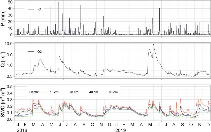
4026                                                                                                        J. Fürst et al.: Rosalia

Figure 4. Gauging site Q4 with 2-ft H-flume, spectrometer device and ISCO autosampler.

snapshot information in case of events. The amount of water             Close to the autosampler, open precipitation samples are
ensures a statistically sound sample size, while the sampling        collected approximately bi-weekly with a totalisator station
interval is short enough to enable the investigation of runoff       (Palmex Ltd., Croatia) which is suitable for isotope sampling
events and is long enough that the autosampler can be left           (Gröning et al., 2012). The sample bottle is inside a plastic
in the field for 24 d without maintenance. The suction tube          pipe and thus protected from direct sunlight. The tube that
leading from the H-flume to the autosampler is occasionally          connects the sample bottle to the funnel outlet has a small di-
affected by frost. The frozen water inside the tube prevents         ameter and extends to the bottom of the sample bottle to limit
the autosampler pump from collecting water samples. Since            air exchange. Since the collected rainfall at Q4 is not affected
the installation of the system, this has happened only rarely        by interception, the samples did not undergo canopy-induced
(less than 20 d), and we plan on further measures to mitigate        changes in the isotopic ratio that can influence the results of
freezing issues arising from small amounts of residual water         hydrologic models (Stockinger et al., 2015). Additionally, a
in the tube that the pump cannot fully flush out. A poten-           Palmex totalisator station was installed at K1 to consider el-
tial evaporation issue arises from the fact that the autosam-        evation effects on isotope ratios and sampled approximately
pler is not a cooled field sampler and the sample bottles are        bi-weekly until September 2020. Since September 2020, the
open to the sampler’s internal atmosphere. Hence, we man-            totalisator has been emptied daily during work days (Monday
ually collected streamflow grab samples in closed high den-          to Friday) by staff of the BOKU education centre.
sity polyethylene (HDPE) bottles each time the field site was           Both δ 18 O and δ 2 H are analysed using laser spectroscopy
visited and measured their isotope ratio within a few days.          (Picarro L2140-i, Picarro Inc., Santa Clara, CA, USA) in
These values were then compared to those of the sampling             the isotope laboratory at BOKU. A calibration with labora-
bottle which was standing the longest in the field. Prelimi-         tory reference material calibrated against the Vienna Stan-
nary results indicated no major evaporation enrichment prob-         dard Mean Ocean Water and Standard Light Antarctic Pre-
lem with a mean difference in δ 18 O of 0.11 ‰ for more than         cipitation scale was used. All values are given in delta nota-
a year of data (measurement uncertainty of 0.1 ‰). Nonethe-          tion, and the precision of the instrument (1σ ) was better than
less, occasionally larger deviations up to 0.4 ‰ were ob-            0.1 ‰ and 0.5 ‰ for δ 18 O and δ 2 H.
served. To minimise possible evaporation effects we adapted
the sampling bottles according to a recent publication (von          4   Data
Freyberg et al., 2020) by placing a 100 mm syringe (with-
out the needle) into the opening of the sampling bottle which        All time series data are recorded, stored and routinely visu-
effectively reduced the area open to atmosphere to a 2 mm            alised using addVANTAGE Pro. For comprehensive analy-
diameter opening (the tip of the syringe body).                      sis, data are regularly exported into the frequently used and

Earth Syst. Sci. Data, 13, 4019–4034, 2021                                           https://doi.org/10.5194/essd-13-4019-2021

J. Fürst et al.: Rosalia                                                                                                    4027

                                                                   at the time of publication, only the years 2018 and 2019 are
                                                                   presented in the graphs below to maintain readability.

                                                                   4.1   Discharge data

                                                                   Raw discharge data at the H-flume gauges Q1, Q2 and Q4
                                                                   needed careful inspection and editing. First, spikes in the hy-
                                                                   drographs (one or two consecutive values significantly ex-
                                                                   ceeding the value before and after the spike) were attributed
                                                                   to random events such as a leave under the ultrasonic depth
                                                                   sensor and were automatically replaced by linear interpola-
                                                                   tion. Next, visually detected implausible discharges were re-
                                                                   placed by linear interpolation when reliably possible or were
                                                                   deleted otherwise. As an example, occasionally during very
                                                                   low flow (water level less than 2 cm in the flume), single
                                                                   leaves can temporarily (a few hours) get stuck at the nar-
                                                                   row outlet of the flume and cause the water level to rise a few
                                                                   millimetres. Such events are clearly visible as plateau-shaped
                                                                   parts of the hydrograph and can be safely replaced by linear
                                                                   interpolation. At these gauges, the measurements have never
                                                                   been disturbed by freezing.
                                                                      At the weir Q3, two issues required editing. (1) During
                                                                   very low flow, leaves and grass can occasionally get stuck at
                                                                   the weir crest, causing the water level to rise. These events
                                                                   can be detected in the images transmitted daily by a surveil-
                                                                   lance camera and visually in the hydrograph. Such artefacts
                                                                   are replaced by linear interpolation. (2) During longer frost
                                                                   periods, the stilling basin may be covered by ice, and there-
Figure 5. HydraProbe sensors installed at site Q2S0.               fore the discharge is no longer described by the weir for-
                                                                   mula. These situations can be detected by visual inspection of
                                                                   the hydrograph and comparison with the temperature. These
freely available time series management system HEC DSS             parts of the records have been deleted.
and the management software HEC DSSVue (Hydrologic                    Discharge is characterised by its wide range of values
Engineering Center, 2010). HEC DSSVue has powerful vi-             (Table 3). At Q3 (watershed outlet with 222 ha), low flows
sualisation features and provides a convenient graphical edi-      in summer and autumn are frequently less than 3 L s−1 ,
tor for the time series. During editing, obvious artefacts such    while peak flows of more than 500 L s−1 have occurred
as spikes generated during maintenance, occasional obstruc-        twice since 2015. Specific discharge does not vary signif-
tions of flumes during storms and similar disturbances are re-     icantly between the four watersheds and typically ranges
moved from the raw data. The data cleaning is specific to the      from 1 to 2 L s−1 km−2 during low to medium flows and up
variables and is therefore discussed in detail in the respective   to 30 L s−1 km−2 during peak flows (calculated from daily
sections below. For even more flexible and automated pro-          means).
cessing, as well as for publication, the HEC DSS database             In the hydrographs for the period 2018 to 2019 (Fig. 6) it
was converted into a simple SQLite database (Hipp et al.,          can be seen that the base flow is greater in spring and early
2019), which provides efficient and simple access from dif-        summer than in autumn and winter and that sharp runoff
ferent software tools, including Python and R (Müller et al.,      peaks occur after rainfall events. The zoomed-in hydrographs
2018).                                                             for July/August 2018 (Fig. 7) illustrate characteristic diurnal
   As the implementation of the instruments started in spring      fluctuations of discharge during no-rain periods in the vege-
2015, the earliest time series are from sites Q1 and Q2 and        tation period (see section “Applications” for more details).
start in May 2015. Until September 2015, rain gauges K1 and
K2, soil water profiles Q1S0 and Q2S0, and stream gauge Q3         4.2   Precipitation data
were also added and are delivering data. Soil water profiles
Q2S1 and Q2S2 were added in April 2016 and rain gauge              For quality control, rainfall data recorded by tipping bucket
K3 and stream gauge Q4 in summer 2018. For the majority            devices (Q1 to Q4) are compared to records of the weigh-
of the data, more than 4 years of records are currently avail-     ing rain gauges and to corresponding hydrographs. They are
able (spring 2021). Out of the 5 years of records available        deleted if the funnel appears to have been (partially) blocked.

https://doi.org/10.5194/essd-13-4019-2021                                         Earth Syst. Sci. Data, 13, 4019–4034, 2021
4028                                                                                                               J. Fürst et al.: Rosalia

Table 3. Statistics of discharge records and of missing data.

                     Site   Time period                  Min discharge     Max discharge     Mean discharge     Percent
                                                               (L s−1 )          (L s−1 )           (L s−1 )    missing
                     Q1     1 Jun 2015–31 Dec 2019                0.05               8.11               0.27        3.3
                     Q2     1 Jun 2015–31 Dec 2019                0.24              12.64               0.81        0.9
                     Q3     1 Sep 2015–31 Dec 2019                1.75             582.34               7.55        6.8
                     Q4     1 Jul 2018–31 Dec 2019                1.35             309.68               4.23        1.1

Figure 6. Discharge hydrographs at gauges Q1 to Q4 for the years 2018–2019 (Q in log scale).

Also, records for the winter season from November to Febru-               rain gauges are useful for analysing storm events as intercep-
ary are excluded due to tipping bucket issues with freezing.              tion reduces rainfall depths by only a small percentage. For
Anomalies observed during field maintenance visits (one to                water balance investigations of periods longer than a week,
two per month) are also considered. The three weighing rain               however, only the gauges not affected by interception should
gauges have provided gap-free records since the time of in-               be used.
stallation up to now, with a resolution of 0.1 mm. For most
rainfall events between March and October, consistent and                 4.3   Soil water data
plausible data were acquired by up to seven rain gauges in
total, providing a high-resolution rainfall pattern for a small           With 14 HydraProbe sensors installed, and each measuring
area of 222 ha and being spread over different altitudes from             six variables, 84 soil-water-related time series at 10 min res-
385 to 655 m a.s.l (Table 4, Fig. 8).                                     olution are recorded, resulting in a large volume of data. In
   In this densely forested watershed, it was not possible to             the data repository, only soil water content (SWC) and soil
place all rain gauges at sites without interception or rain-              temperature are provided. Apart from an initial power supply
shading. However, the rainfall depths at the seven sites are              problem at Q2S2, these sensors worked without any problem
very similar for events that cover the entire catchment. Gauge            or data loss and required no maintenance. Figure 9 illustrates
Q1 is affected by interception, which amounts to typically                daily SWC in four depths at profile Q2S0, together with daily
less than 2 mm per event (compared to weighing rain gauges                rainfall data. It is important to mention that the installation of
K1 and K2), but monthly precipitation at Q1 is on average                 the sensors requires digging a trench, which causes consid-
only 75 % of the mean of K1 and K2. At Q2, monthly pre-                   erable local disturbance of the soil. Despite careful refilling,
cipitation is on average 87 % of the mean of K1 and K2. (K1               local infiltration paths could be influenced, and data do not
is close to the highest elevation of the watershed, K2 at the             necessarily reflect natural conditions for some time after in-
lowest; see Fig. 1 and Table 1.) Therefore, the data from all             stallation. During the first few months after installation, for
                                                                          example, deeper probes reacted faster to rainfall than those

Earth Syst. Sci. Data, 13, 4019–4034, 2021                                                  https://doi.org/10.5194/essd-13-4019-2021
J. Fürst et al.: Rosalia 4029
Figure 7. Diurnal fluctuations of flow for July/August 2018 (peak flows are cut off: Q1 and Q2 at 0.8 L s−1 ; Q3 and Q4 at 10 L s−1 ).
Table 4. Statistics of precipitation data (statistics are calculated only if there are no missing values in the interval). NA – not available
Site Time Percent Max daily Annual precipitation
period missing precip. (mm) (mm)
2016 2017 2018 2019
K1 26 Aug 2015–31 Dec 2019 0 69.2 975 676 877 759
K2 26 Aug 2015–31 Dec 2019 0 60.8 949 682 906 739
K3 1 Aug 2018–31 Dec 2019 0 84.1 NA NA NA 737
Q1 1 Jun 2015–31 Dec 2019 26 56.6 NA NA NA NA
Q2 1 Jun 2015–31 Dec 2019 29 63.0 NA NA NA NA
Q3 1 Sep 2015–31 Dec 2019 31 48.6 NA NA NA NA
Q4 1 Jul 2018–31 Dec 2019 23 27.0 NA NA NA NA
close to the surface (Fig. 10). This can be attributed to artifi- 4.5 Isotopic data
cial flow paths along the walls of the trench and the cables,
or to effects arising from interrupted and destroyed natural At discharge site Q4, river and precipitation samples have
macropores like wormholes. However, direct effects due to been collected since June and October 2019, respectively
installation practically disappeared after the first season. (Fig. 11). The precipitation data are collected as bi-weekly
bulk samples and are compared to the daily river water grab
4.4 Electrical conductivity and temperature of runoff samples. The comparison shows the response of the dis-
charge to the precipitation input tracer signal (Fig. 11). Fur-
At discharge sites Q1, Q2 and Q4, water temperature and thermore, the precipitation and river water isotopes vary sea-
electrical conductivity are measured. Due to the risk of dam- sonally, with larger values in summer and lower values in
age by frost, the sensors are removed during the frost pe- winter months. This seasonality originated from contribu-
riod from December to March at sites Q1 and Q2. Besides tions of precipitation to discharge, and isotope ratios in pre-
frost, conductivity records at sites Q1 and Q2 are additionally cipitation seasonally vary due to changes in temperature,
negatively influenced by the sensor problems described in sources of vapour for cloud formation and different rain-out
Sect. 3.2. Regular conductivity measurements with a portable histories (Feng et al., 2009). Apart from this, there are some
device showed that the conductivity of base flow is stable at preliminary indications of different flow paths, such as base
sites Q1 and Q2 (typically approx. 120 µS cm−1 ) so that the flow (relatively stable δ 18 O isotope values around −10 ‰),
recorded conductivity series are still informative for the sep- interflow (moderate increases or decreases in isotopes, for
aration of base flow and direct runoff events despite conduc- example, at the beginning of August 2019), and faster flow
tivity offsets in the records. (sharp peaks), suggesting dynamic runoff processes and tran-
https://doi.org/10.5194/essd-13-4019-2021 Earth Syst. Sci. Data, 13, 4019–4034, 20214030 J. Fürst et al.: Rosalia
Figure 8. Daily rainfall at the weighing rain gauges for 2018 to 2019.
Figure 9. Daily soil water content and corresponding daily rainfall and log-discharge at site Q2S0 for 2018 to 2019.
sit times in the Rosalia watershed, which will be analysed in DEMs, watershed divides and the drainage network were de-
the future. rived in GIS. Additionally, a ground survey was performed
for the main creeks in 2018. These data are included in the
repository in shapefile format.
4.6 Spatial data
Data interpretation is complemented by a comprehensive 5 Applications
amount of spatial data characterising the site. DEMs at var-
ious resolutions are available, including a 10 × 10 m DEM The presented data are suitable for studying processes of wa-
(data source: Land Niederösterreich – http://data.noe.gv. ter flow and transport in small, forested watersheds. They
at, last access: 29 June 2021) and a lidar-based DEM at have been used in academic teaching and research. The site
0.5 × 0.5 m (Immitzer, 2009), accessible at https://zenodo. is regularly used for advanced field courses in the water man-
org/record/4601057 (last access: 29 June 2021). From these agement and environmental engineering curriculum. During
Earth Syst. Sci. Data, 13, 4019–4034, 2021 https://doi.org/10.5194/essd-13-4019-2021J. Fürst et al.: Rosalia 4031
Figure 10. Detail of daily soil water content at site Q2S1: deeper sensors reacted faster to rainfall on 12 May 2016.
discharge and rainfall records at site Q2, the model also used
soil moisture data at sites Q2S0, Q2S1 and Q2S2.
Wesemann (2021) investigated the influence of forest
roads and skid trails on runoff during heavy rainfall events in
the Rosalia catchment. Based on the 0.5 × 0.5 m lidar DEM
(Immitzer, 2009), he reconstructed a historical terrain model
without forest roads and buildings, which allowed the com-
parison of the runoff from the natural terrain surface and
runoff from the current surface where flow paths are mod-
Figure 11. Precipitation and river water δ 18 O isotopes at site Q4.
ified by the forest roads. The physically based rainfall-runoff
model RoGeR (Steinbrich et al., 2016) was set up for the
catchment to quantify the influence of the road network on
the runoff behaviour for three flood events observed at gauge
these courses, students not only learn about the setup and op- Q3 between 2017 and 2019. Rainfall data from all seven rain
eration of a hydrological monitoring network, but they also gauges were used to assess the effect of the spatio-temporal
contribute to the improvement of knowledge about the water- distribution of rainfall on runoff.
shed by collecting and analysing soil samples or performing
validation measurements of the instruments. 6 Data availability
The dataset provided the majority of the database for two
master’s theses and a dissertation. Irsigler (2017) applied dis- All time series data were cleaned of the most obvi-
charge and electrical conductivity data in a simple two-end- ous errors and artefacts and stored in an easily useable
member mixing model for the separation of base flow and database. In addition, some auxiliary spatial datasets are
direct runoff, using an approach described by Lott and Stew- made available. The data described above are available at
art (2016). Stecher (2021) investigated a phenomenon that https://doi.org/10.5281/zenodo.3997140 (Fürst et al., 2020).
is observed in no-rain periods during the vegetation period: This repository comprises an SQLite database file with all
daily fluctuations of discharge, with peaks at 08:00 CET up the high-resolution time series data, an MS Excel sheet with
to 40 % higher than the minimum at 17:00 CET, occur consis- the isotopic data and the spatial datasets. Usage of the data is
tently at all four gauging sites. It was hypothesised that this described by a comprehensive HTML file (generated by an
is an effect of forest transpiration since these diurnal fluc- R Markdown document also included), which includes pre-
tuations are not observed from late autumn to early spring. views and a full technical description of the data, including R
By modelling a slope transect at site Q2 with HYDRUS 2D code chunks to read and visualise them. The data repository
(Simunek et al., 1999), the diurnal fluctuations of discharge will be updated annually.
are demonstrated to be caused by the vegetation in the ripar-
ian zone within only a few metres of the creek. Besides the
https://doi.org/10.5194/essd-13-4019-2021 Earth Syst. Sci. Data, 13, 4019–4034, 20214032 J. Fürst et al.: Rosalia
7 Summary References
The data presented in this article represent an effort to mea-
Anderson, S. P., Bales, R. C., and Duffy, C. J.: Critical Zone
sure components of the energy and water cycle in a forested
Observatories: Building a network to advance interdisciplinary
catchment in the eastern Austrian Alps. The period of record study of Earth surface processes, Mineral. Mag., 72, 7–10,
for precipitation, discharge, air and water temperature, rel- https://doi.org/10.1180/minmag.2008.072.1.7, 2018.
ative humidity, electrical conductivity, and soil water con- Bernhardt, M., Schulz, K., and Pomeroy, J. W.: The International
tent started in 2015. Water quality monitoring and sampling Network for Alpine Research Catchment Hydrology: A new
for precipitation and river water δ 18 O isotopes were added GEWEX crosscutting Project, Hydrol. Wasserbewirts., 59, 190–
in 2018 and 2019. Measurements use consistent methods 191, 2015.
to ensure comparability within the research catchment. The Blöschl, G., Blaschke, A. P., Broer, M., Bucher, C., Carr, G., Chen,
data have proven fit for the purpose of supporting hydrolog- X., Eder, A., Exner-Kittridge, M., Farnleitner, A., Flores-Orozco,
ical and hydro-meteorological process research. Making the A., Haas, P., Hogan, P., Kazemi Amiri, A., Oismüller, M., Para-
data available to the research and applied hydrology com- jka, J., Silasari, R., Stadler, P., Strauss, P., Vreugdenhil, M., Wag-
ner, W., and Zessner, M.: The Hydrological Open Air Laboratory
munities has two main objectives. First, it intends to inform
(HOAL) in Petzenkirchen: a hypothesis-driven observatory, Hy-
decision-makers in the Rosalia forest. The record is an im- drol. Earth Syst. Sci., 20, 227–255, https://doi.org/10.5194/hess-
portant source of baseline data that can be used to assess 20-227-2016, 2016.
the effect of disturbances such as clear-cuts and changing Blöschl, G., Bierkens, M. F. P., Chambel, A., Cudennec, C.,
forestry on hydrological processes. Second, these data are Destouni, G., Fiori, A., Kirchner, J. W., McDonnell, J. J.,
provided to allow others to also investigate hydrological pro- Savenije, H. H. G., Sivapalan, M., Stumpp, C., Toth, E., Volpi,
cesses, medium-term patterns and potential changes in this E., Carr, G., Lupton, C., Salinas, J., Széles, B., Viglione, A., Ak-
type of watershed. soy, H., Allen, S. T., Amin, A., Andréassian, V., Arheimer, B.,
Aryal, S. K., Baker, V., Bardsley, E., Barendrecht, M. H., Bar-
tosova, A., Batelaan, O., Berghuijs, W. R., Beven, K., Blume,
Author contributions. JF was involved in field work to collect T., Bogaard, T., Borges de Amorim, P., Böttcher, M. E., Boulet,
the data discussed here, including selection and installation of G., Breinl, K., Brilly, M., Brocca, L., Buytaert, W., Castellarin,
the instruments, processing, quality assurance, and quality control. A., Castelletti, A., Chen, X., Chen, Y., Chen, Y., Chifflard, P.,
HPN and KS handled strategic decisions and funding. JG provided Claps, P., Clark, M. P., Collins, A. L., Croke, B., Dathe, A.,
advice on site selection and provided some spatial data. RN han- David, P. C., de Barros, F. P. J., de Rooij, G., Di Baldassarre, G.,
dled the selection and installation of soil sensors. MS and CS set up Driscoll, J. M., Duethmann, D., Dwivedi, R., Eris, E., Farmer,
the isotope measurement network and maintain it. All the authors W. H., Feiccabrino, J., Ferguson, G., Ferrari, E., Ferraris, S., Fer-
contributed to writing the manuscript. sch, B., Finger, D., Foglia, L., Fowler, K., Gartsman, B., Gas-
coin, S., Gaume, E., Gelfan, A., Geris, J., Gharari, S., Gleeson,
T., Glendell, M., Gonzalez Bevacqua, A., González-Dugo, M.
P., Grimaldi, S., Gupta, A. B., Guse, B., Han, D., Hannah, D.,
Competing interests. The authors declare that they have no con-
Harpold, A., Haun, S., Heal, K., Helfricht, K., Herrnegger, M.,
flict of interest. Names of products and companies are only men-
Hipsey, M., Hlaváčiková, H., Hohmann, C., Holko, L., Hopkin-
tioned for better understanding and traceability; none of the authors
son, C., Hrachowitz, M., Illangasekare, T. H., Inam, A., Inno-
are associated with any of the mentioned companies.
cente, C., Istanbulluoglu, E., Jarihani, B., Kalantari, Z., Kalvans,
A., Khanal, S., Khatami, S., Kiesel, J., Kirkby, M., Knoben,
W., Kochanek, K., Kohnová, S., Kolechkina, A., Krause, S.,
Disclaimer. Publisher’s note: Copernicus Publications remains Kreamer, D., Kreibich, H., Kunstmann, H., Lange, H., Liber-
neutral with regard to jurisdictional claims in published maps and ato, M. L. R., Lindquist, E., Link, T., Liu, J., Loucks, D. P.,
institutional affiliations. Luce, C., Mahé, G., Makarieva, O., Malard, J., Mashtayeva, S.,
Maskey, S., Mas-Pla, J., Mavrova-Guirguinova, M., Mazzoleni,
M., Mernild, S., Misstear, B. D., Montanari, A., Müller-Thomy,
Acknowledgements. Over the years, several people have con- H., Nabizadeh, A., Nardi, F., Neale, C., Nesterova, N., Nurtaev,
tributed to the implementation of the Rosalia test site, the oper- B., Odongo, V. O., Panda, S., Pande, S., Pang, Z., Papachar-
ation of the instruments and data collection and deserve recogni- alampous, G., Perrin, C., Pfister, L., Pimentel, R., Polo, M. J.,
tion. These include Wisam Almohamed, Matthias Bernhardt, Lau- Post, D., Prieto Sierra, C., Ramos, M.-H., Renner, M., Reynolds,
rin Bonell, Reinhard Burgholzer, Roman Eque, Heinz Fassl, Martin J. E., Ridolfi, E., Rigon, R., Riva, M., Robertson, D. E., Rosso,
Hackl, Mathew Herrnegger, Freddy Kratzert, Thomas Lehner, Mar- R., Roy, T., Sá, J. H. M., Salvadori, G., Sandells, M., Schaefli,
tin Lichtblau, Johann Karner, Philipp Proksch, Andreas Schwen, B., Schumann, A., Scolobig, A., Seibert, J., Servat, E., Shafiei,
Wolfgang Sokol, Gabriel Stecher and Johannes Wesemann. M., Sharma, A., Sidibe, M., Sidle, R. C., Skaugen, T., Smith, H.,
Spiessl, S. M., Stein, L., Steinsland, I., Strasser, U., Su, B., Szol-
gay, J., Tarboton, D., Tauro, F., Thirel, G., Tian, F., Tong, R., Tus-
Review statement. This paper was edited by Lukas Gudmunds- supova, K., Tyralis, H., Uijlenhoet, R., van Beek, R., van der Ent,
son and reviewed by two anonymous referees. R. J., van der Ploeg, M., Van Loon, A. F., van Meerveld, I., van
Earth Syst. Sci. Data, 13, 4019–4034, 2021 https://doi.org/10.5194/essd-13-4019-2021J. Fürst et al.: Rosalia 4033 Nooijen, R., van Oel, P. R., Vidal, J.-P., von Freyberg, J., Voro- istry and structure, J. Appl. Remote Sens., 4, 043510, gushyn, S., Wachniew, P., Wade, A. J., Ward, P., Westerberg, I. https://doi.org/10.1117/1.3361375, 2010. K., White, C., Wood, E. F., Woods, R., Xu, Z., Yilmaz, K. K., and Laudon, H., Taberman, I., Ågren, A., Futter, M., Ottosson- Zhang, Y.: Twenty-three unsolved problems in hydrology (UPH) Löfvenius, M., and Bishop, K.: The Krycklan Catchment Study – a community perspective, Hydrolog. Sci. J., 64, 1141–1158, – A flagship infrastructure for hydrology, biogeochemistry, and https://doi.org/10.1080/02626667.2019.1620507, 2019. climate research in the boreal landscape, Water Resour. Res., 49, Bogena, H. R., White, T., Bour, O., Li, X., and Jensen, K. H.: 7154–7158, https://doi.org/10.1002/wrcr.20520, 2013. Toward Better Understanding of Terrestrial Processes through Leitner, S., Minixhofer, P., Inselsbacher, E., Keiblinger, K. M., Long-Term Hydrological Observatories, Vadose Zone J., 17, 1– Zimmermann, M., and Zechmeister-Boltenstern, S.: Short-term 10, https://doi.org/10.2136/vzj2018.10.0194, 2018. soil mineral and organic nitrogen fluxes during moderate and Cosby, J. and Emmett, B.: Plynlimon Experimental Catch- severe drying–rewetting events, Appl. Soil Ecol., 114, 28–33, ments: available at: https://www.ceh.ac.uk/our-science/projects/ https://doi.org/10.1016/j.apsoil.2017.02.014, 2017. plynlimon-experimental-catchments, last access: 28 May 2020. Lott, D. A. and Stewart, M. T.: Base flow separation: A comparison ESFRI: Roadmap & Strategy Report on Research Infras- of analytical and mass balance methods, J. Hydrol., 535, 525– tructures: available at: http://roadmap2018.esfri.eu/media/1066/ 533, https://doi.org/10.1016/j.jhydrol.2016.01.063, 2016. esfri-roadmap-2018.pdf, last access: 28 May 2020. LTER Network Office: LTER History, available at: https://lternet. Feng, X., Faiia, A. M., and Posmentier, E. S.: Seasonality of iso- edu/network-organization/lter-a-history/, last access: 28 May topes in precipitation: A global perspective, J. Geophys. Res.- 2020. Atmos., 114, D08116, https://doi.org/10.1029/2008JD011279, Morgenschweis, G.: Hydrometrie – Theorie und Praxis der Durch- 2009. flussmessung in offenen Gerinnen, Springer-Verlag, Berlin Hei- Fürst, J., Nachtnebel, H. P., Gasch, J., Nolz, R., Stockinger, delberg, 582 pp., 2010. M. P., Stumpp, C., and Schulz, K.: Rosalia: an exper- Müller, K., Wickham, H., James, D. A., and Falcon, S.: RSQLite: imental research site to study hydrological processes in “SQLite” Interface for R. R package version 2.1.1, available at: a forest catchment – data repository, Zenodo [data set], https://CRAN.R-project.org/package=RSQLite (last access: 29 https://doi.org/10.5281/zenodo.3997141, 2020. June 2021), 2018. Gröning, M., Lutz, H. O., Roller-Lutz, Z., Kralik, M., Gourcy, Neal, C., Reynolds, B., Norris, D., Kirchner, J. W., Neal, M., Row- L., and Pöltenstein, L.: A simple rain collector preventing wa- land, P., Wickham, H., Harman, S., Armstrong, L., Sleep, D., ter re-evaporation dedicated for δ18O and δ2H analysis of cu- Lawlor, A., Woods, C., Williams, B., Fry, M., Newton, G., and mulative precipitation samples, J. Hydrol., 448–449, 195–200, Wright, D.: Three decades of water quality measurements from https://doi.org/10.1016/j.jhydrol.2012.04.041, 2012. the Upper Severn experimental catchments at Plynlimon, Wales: Haberl, H., Winiwarter, V., Andersson, K., Ayres, R. U., Boone, an openly accessible data resource for research, modelling, en- C., Castillo, A., Cunfer, G., Fischer-Kowalski, M., Freuden- vironmental management and education, Hydrol. Process., 25, burg, W. R., Furman, E., Kaufmann, R., Krausmann, F., Langth- 3818–3830, https://doi.org/10.1002/hyp.8191, 2011. aler, E., Lotze-Campen, H., Mirtl, M., Redman, C. L., Reen- Netherer, S., Matthews, B., Katzensteiner, K., Blackwell, E., Hen- berg, A., Wardell, A., Warr, B., and Zechmeister, H.: From schke, P., Hietz, P., Pennerstorfer, J., Rosner, S., Kikuta, S., LTER to LTSER: Conceptualizing the Socioeconomic Dimen- Schume, H., and Schopf, A.: Do water-limiting conditions pre- sion of Long-term Socioecological Research, Ecol. Soc., 11, 13, dispose Norway spruce to bark beetle attack?, New Phytol., 205, https://doi.org/10.5751/ES-01786-110213, 2006. 1128–1141, https://doi.org/10.1111/nph.13166, 2015. Hipp, D. R., Kennedy, D., and Mistachkin, J.: SQLite SQLite De- Porporato, A. and Rodriguez-Iturbe, I.: Ecohydrology- velopment Team, available at: https://www.sqlite.org/download. a challenging multidisciplinary research perspec- html (last access: 29 June 2021), 2019. tive/Ecohydrologie: une perspective stimulante de recherche Holzmann, H.: Status and perspectives of hydrological research in multidisciplinaire, Hydrolog. Sci. J., 47, 811–821, small basins in Europe, Geographical Research Letters, 44, 601– https://doi.org/10.1080/02626660209492985, 2002. 614, https://doi.org/10.18172/cig.3406, 2018. Schumann, S., Schmalz, B., Meesenburg, H., and Schröder, U.: Sta- Hydrologic Engineering Center: HEC DSSVue Version 2.0, US tus and Perspectives of Hydrology in Small Basins – Results Army Corps of Engineers, Institute for Water Resources, Davis, and recommendations of the International Workshop in Goslar- CA, 2010. Hahnenklee, Germany, 2009 and Inventory of Small Hydrolog- Immitzer, M.: Auswertung von Airborne-Laser-Scanning-Daten für ical Research Basins, German National Committee for the In- die Ableitung des Holzvorrates im Lehrforst der Universität für ternational Hydrological Programme (IHP) of UNESCO and the Bodenkultur, MSc thesis, University of Natural Resources and Hydrology and Water Resources Programme (HWRP) of WMO Life Sciences Vienna, Vienna, 163 pp., 2009. KoblenzIHP/HWRP-Berichte, Heft 10, 71 pp., 2010. Irsigler, S. Z.: Nutzung von Leitfähigkeits- und Temperaturdaten Schwen, A., Zimmermann, M., Leitner, S., and Woche, S. zur verbesserten Beschreibung der Abflussprozesse in kleinen K.: Soil Water Repellency and its Impact on Hydraulic bewaldeten Einzugsgebieten, MSc thesis, Wasser – Atmosphäre Characteristics in a Beech Forest under Simulated Cli- – Umwelt, Universität für Bodenkultur Wien, Wien, 128 pp., mate Change, Vadose Zone J., 14, vzj2015.2006.0089, 2017. https://doi.org/10.2136/vzj2015.06.0089, 2015. Kampe, T., Johnson, B., Kuester, M., and Keller, M.: NEON: Seyfried, M., Lohse, K., Marks, D., Flerchinger, G., Pierson, F., the first continental-scale ecological observatory with and Holbrook, W. S.: Reynolds Creek Experimental Watershed airborne remote sensing of vegetation canopy biochem- https://doi.org/10.5194/essd-13-4019-2021 Earth Syst. Sci. Data, 13, 4019–4034, 2021
You can also read