GWL_FCS30: a global 30 m wetland map with a fine classification system using multi-sourced and time-series remote sensing imagery in 2020 - ESSD
←
→
Page content transcription
If your browser does not render page correctly, please read the page content below

Earth Syst. Sci. Data, 15, 265–293, 2023
https://doi.org/10.5194/essd-15-265-2023
© Author(s) 2023. This work is distributed under
the Creative Commons Attribution 4.0 License.

            GWL_FCS30: a global 30 m wetland map with a fine
             classification system using multi-sourced and
              time-series remote sensing imagery in 2020
       Xiao Zhang1,2 , Liangyun Liu1,2,3 , Tingting Zhao1,4 , Xidong Chen5 , Shangrong Lin6 , Jinqing Wang1,2,3 ,
                                             Jun Mi1,2,3 , and Wendi Liu1,2,3
          1 InternationalResearch Center of Big Data for Sustainable Development Goals, Beijing 100094, China
                   2 Key Laboratory of Digital Earth Science, Aerospace Information Research Institute,
                                    Chinese Academy of Sciences, Beijing 100094, China
           3 School of Electronic, Electrical and Communication Engineering, University of Chinese Academy of

                                               Sciences, Beijing 100049, China
                 4 College of Geomatics, Xi’an University of Science and Technology, Xi’an 710054, China
                5 North China University of Water Resources and Electric Power, Zhengzhou 450046, China
      6 School of Atmospheric Sciences, Southern Marine Science and Engineering Guangdong Laboratory (Zhuhai),

                                 Sun Yat-sen University, Zhuhai 519082, Guangdong, China
                                    Correspondence: Liangyun Liu (liuly@radi.ac.cn)

                                  Received: 24 May 2022 – Discussion started: 19 August 2022
                     Revised: 21 December 2022 – Accepted: 27 December 2022 – Published: 17 January 2023

      Abstract. Wetlands, often called the “kidneys of the earth”, play an important role in maintaining ecological
      balance, conserving water resources, replenishing groundwater and controlling soil erosion. Wetland mapping
      is very challenging because of its complicated temporal dynamics and large spatial and spectral heterogeneity.
      An accurate global 30 m wetland dataset that can simultaneously cover inland and coastal zones is lacking. This
      study proposes a novel method for wetland mapping by combining an automatic sample extraction method, ex-
      isting multi-sourced products, satellite time-series images and a stratified classification strategy. This approach
      allowed for the generation of the first global 30 m wetland map with a fine classification system (GWL_FCS30),
      including five inland wetland sub-categories (permanent water, swamp, marsh, flooded flat and saline) and three
      coastal tidal wetland sub-categories (mangrove, salt marsh and tidal flats), which was developed using Google
      Earth Engine platform. We first combined existing multi-sourced global wetland products, expert knowledge,
      training sample refinement rules and visual interpretation to generate large and geographically distributed wet-
      land training samples. Second, we integrated the Landsat reflectance time-series products and Sentinel-1 syn-
      thetic aperture radar (SAR) imagery to generate various water-level and phenological information to capture the
      complicated temporal dynamics and spectral heterogeneity of wetlands. Third, we applied a stratified classifi-
      cation strategy and the local adaptive random forest classification models to produce the wetland dataset with
      a fine classification system at each 5◦ × 5◦ geographical tile in 2020. Lastly, GWL_FCS30, mosaicked by 961
      5◦ × 5◦ regional wetland maps, was validated using 25 708 validation samples, which achieved an overall ac-
      curacy of 86.44 % and a kappa coefficient of 0.822. The cross-comparisons with other global wetland products
      demonstrated that the GWL_FCS30 dataset performed better in capturing the spatial patterns of wetlands and had
      significant advantages over the diversity of wetland sub-categories. The statistical analysis showed that the global
      wetland area reached 6.38 million km2 , including 6.03 million km2 of inland wetlands and 0.35 million km2 of
      coastal tidal wetlands, approximately 72.96 % of which were distributed poleward of 40◦ N. Therefore, we can
      conclude that the proposed method is suitable for large-area wetland mapping and that the GWL_FCS30 dataset
      is an accurate wetland mapping product that has the potential to provide vital support for wetland manage-

Published by Copernicus Publications.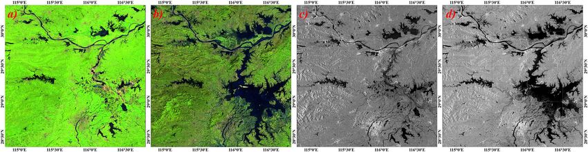
266                                                 X. Zhang et al.: Global 30 m wetland map with fine classification system

       ment. The GWL_FCS30 dataset in 2020 is freely available at https://doi.org/10.5281/zenodo.7340516 (Liu et
       al., 2022).

1   Introduction                                                  (WorldCover; Zanaga et al., 2021; Dynamic World; Brown
                                                                  et al., 2022; and FROM_GLC10; Gong et al., 2019), contain-
                                                                  ing an independent wetland layers, were produced, but their
The Ramsar Convention defines wetlands as “areas of marsh,
                                                                  classification algorithms were not specifically designed for
fen, peatland or water, whether natural or artificial, perma-
                                                                  the wetland environment, so wetlands usually suffered from
nent or temporary, with water that is static or flowing, fresh,
                                                                  low accuracy in these products. In addition, several global
brackish or salt, including areas of marine water the depth of
                                                                  coastal tidal wetland products have been developed, includ-
which at low tide does not exceed six meters” (Gardner and
                                                                  ing the global mangrove extent (Bunting et al., 2018; Hamil-
Davidson, 2011). Wetlands not only provide humans with
                                                                  ton and Casey, 2016) and global 30 m tidal flat datasets from
a large amount of food, raw materials and water resources
                                                                  1984 to 2016 (Murray et al., 2019), but these only covered
(Ludwig et al., 2019; Z. Zhang et al., 2022) but also play an
                                                                  the intertidal zones. Thus, an accurate global 30 m thematic
important role in maintaining ecological balance, conserving
                                                                  wetland dataset, with fine wetland categories and covering
water resources, replenishing groundwater and controlling
                                                                  both inland and coastal zones, is still lacking.
soil erosion (Hu et al., 2017a; Mao et al., 2021; Wang et al.,
                                                                     One of the largest challenges of current state-of-the-art
2020; Zhu and Gong, 2014). Therefore, they are also called
                                                                  methods for large-area wetland mapping is to collect a mas-
the “kidneys of the earth” (Guo et al., 2017). However, due
                                                                  sive number of training samples (Liu et al., 2021; Ludwig et
to increasing human activities, including agriculturalization,
                                                                  al., 2019). Zhang et al. (2021b) mentioned two options for
industrialization and urbanization (McCarthy et al., 2018; Xi
                                                                  collecting training samples, including the visual interpreta-
et al., 2020), and climatic changes, such as sea-level rise and
                                                                  tion method and deriving training samples from pre-existing
coastal erosion (Cao et al., 2020; Wang et al., 2021), wet-
                                                                  products. First, since the visual interpretation method had
lands have been seriously degraded and threatened over the
                                                                  significant advantages over the confidence of training sam-
past few decades (Mao et al., 2020). Thus, having access to
                                                                  ples, it was widely used for local or regional wetland map-
timely and accurate wetland mapping information is pivotal
                                                                  ping (Amani et al., 2019; Wang et al., 2020). However, col-
for protecting biodiversity and supporting the sustainable de-
                                                                  lecting accurate and sufficient training samples is usually a
velopment goals.
                                                                  time-consuming process and involves a large amount of man-
   Along with the rapid development of remote sensing tech-
                                                                  ual work, so it was impractical and nearly impossible to use
niques and computing abilities, a variety of regional and
                                                                  the visual interpretation for collecting global wetland sam-
global wetland datasets have been produced with spatial res-
                                                                  ples. Comparatively, the process of deriving training sam-
olutions ranging from 30 m to 1◦ (∼ 112 km) (Chen et al.,
                                                                  ples from existing products and applying some rules or re-
2022; Gumbricht et al., 2017; Lehner and Döll, 2004; Mao
                                                                  finement methods to identify these high-confidence samples
et al., 2020; Matthews and Fung, 1987; Tootchi et al., 2019).
                                                                  from existing products shows promise (Zhang et al., 2021b).
Recently, Tootchi et al. (2019) and Hu et al. (2017a) have sys-
                                                                  So this approach is practical in that it could quickly produce a
tematically reviewed the generation process of global wet-
                                                                  large and geographically diverse distribution of training sam-
land datasets with various spatial and temporal resolutions
                                                                  ples without much manual effort. Thus, the second option at-
and wetland categories and found significant uncertainties
                                                                  tracted increasing attention and has been successfully used
and inconsistencies among these datasets. For example, the
                                                                  for large-area land-cover mapping (Zhang and Roy, 2017;
global total wetland area reviewed by Hu et al. (2017a)
                                                                  Zhang et al., 2020, 2021b). For example, Zhang et al. (2021b)
ranged from 2.12 to 7.17 million km2 based on remote sens-
                                                                  used global training samples derived from the combination
ing products. Therefore, great uncertainties among global
                                                                  of the CCI_LC and MCD43A4 Distribution Function Ad-
wetland datasets directly hindered wetland applications and
                                                                  justed Reflectance (NBAR) datasets to produce a global 30 m
analysis. Furthermore, from the perspective of spatial reso-
                                                                  land-cover product with a fine classification system in 2015
lution, although many wetland products have been produced
                                                                  and 2020 (GLC_FCS30) with an overall accuracy of 82.5 %.
at regional or global scales using various remote sensing im-
                                                                  Therefore, if we take effective measures to fuse these existing
agery and different methods (Guo et al., 2017; Tootchi et al.,
                                                                  products and then derive high-confidence training samples
2019), most of them were coarse-spatial-resolution datasets,
                                                                  using some refinement rules, the deriving approach would
ranging from 100 m to 25 km. Recently, with the improve-
                                                                  hold great potential for global wetland mapping.
ment in computing power and storage abilities, three global
                                                                     Another major challenge inherent to wetland mapping is
30 m land-cover products (including GlobeLand30; Chen et
                                                                  the complicated temporal dynamics and the spatial and spec-
al., 2015; FROM_GLC; Gong et al., 2013; and GLC_FCS30;
                                                                  tral heterogeneity. The spectral characteristics of the wet-
Zhang et al., 2021b) and several 10 m land-cover products

Earth Syst. Sci. Data, 15, 265–293, 2023                                           https://doi.org/10.5194/essd-15-265-2023
X. Zhang et al.: Global 30 m wetland map with fine classification system                                                     267

lands would quickly change with the seasonal or daily water        of 2020 via the Google Earth Engine platform for minimiz-
levels of the underlying surface (Ludwig et al., 2019; Mah-        ing the influence of frequent cloud contamination in the trop-
dianpari et al., 2020). Therefore, many studies proposed to        ics and snow and ice in the high latitudes. To minimize the
combine multi-sourced, time-series remote sensing imagery          effect of atmosphere, each Landsat image was atmospheri-
to capture the spatial extent and temporal dynamics of wet-        cally corrected to the surface reflectance by the United States
lands (LaRocque et al., 2020; Ludwig et al., 2019; Murray et       Geological Survey using the Land Surface Reflectance Code
al., 2019; Wang et al., 2021; Z. Zhang et al., 2022). For ex-      (LaSRC) method (Vermote et al., 2016) and then archived
ample, Z. Zhang et al. (2022) and Murray et al. (2019) used        on the Google Earth Engine (GEE) platform. These “bad-
the Landsat time-series imagery to generate tidal-level and        quality” observations (shadow, cloud, snow and saturated
phenological features for identifying coastal tidal wetlands       pixels) in Landsat imagery were masked using the CFmask
and successfully produced the coastal tidal wetlands in China      cloud detection method, which built a series of decision
with an overall accuracy of 97.2 % (Z. Zhang et al., 2022)         rules, using temperature, spectral variability, brightness and
and global trajectory tidal flats with the overall map accuracy    geometric relationship between cloud and shadow, to identify
of 82.3 % (Murray et al., 2019). Except for optical imagery,       these “poor-quality” pixels and achieved the overall accuracy
synthetic aperture radar (SAR) data, which were sensitive to       of 96.4 % (Zhu et al., 2015; Zhu and Woodcock, 2012). In
soil moisture, vegetation structure and inundation, enabled        this study, six optical bands, including blue, green, red, NIR
data acquisition regardless of solar illumination, clouds or       (near infrared), SWIR1 (shortwave infrared 1) and SWIR2
haze and were also widely used for wetland mapping, espe-          (shortwave infrared 2) bands, were used for wetland map-
cially after the Sentinel-1 data became open-access (Li et al.,    ping. In total, 764 239 Landsat scenes were collected to cap-
2020; Slagter et al., 2020; Zhang et al., 2018). For example,      ture various water-level and phenological features according
Li et al. (2020) used the Sentinel-1 time-series imagery to        to the spectral characteristics of various land-cover types,
discriminate wetlands with and without trees and achieved          presented in Sect. 4. Figure 1a illustrates the spatial distri-
an overall accuracy of 86.0 ± 0.2 %. Therefore, the fusion of      bution of all clear-sky observations for all Landsat scenes,
multi-sourced and time-series remote sensing imagery is vi-        and it can be seen that there were more than 10 clear observa-
tal for accurate wetland mapping.                                  tions after masking these “poor-quality” observations in each
   Due to the complicated temporal dynamics and the spa-           region and even in the tropics.
tial and spectral heterogeneity of wetlands, there are very           Then, the Sentinel-1 SAR data, which were demonstrated
few global thematic wetland datasets covering both inland          to be sensitive to the soil moisture, vegetation structure
and coastal regions with a fine classification system and          and inundation information (Li et al., 2020), used dual-
high spatial resolution, which also cause global 30 m wet-         polarization C-band backscatter coefficients to measure the
land mapping with a fine classification system to remain a         incident microwave radiation scattered by the land surface
challenging task. In this study, we combined several exist-        (Torres et al., 2012). This study obtained the Sentinel-1 time-
ing wetland products and multi-sourced time-series remote          series imagery archived on the GEE platform in 2020 in
sensing imagery to (1) derive large and geographically dis-        Interferometric Wide swath mode with a dual-polarization
tributed wetland training samples from pre-existing multi-         of VV and VH. Notably, all Sentinel-1 SAR imagery on
sourced global wetland products to minimize the manual             the GEE platform has been pre-processed by the Sentinel-
participation; (2) develop a robust method to capture the          1 Toolbox with thermal noise removal, radiometric calibra-
temporal dynamics of wetlands and then produce the first           tion and terrain correction using 30 m elevation data (Veci
global 30 m wetland dataset with a fine classification sys-        et al., 2014). Figure 1b also illustrates the spatial distribu-
tem (GWL_FCS30); and (3) quantitatively analyze the spa-           tion of all available Sentinel-1 SAR imagery; there were
tial distribution of different wetland categories and assess the   enough Sentinel-1 SAR observations in each area to cap-
accuracy of GWL_FCS30 in 2020.                                     ture the water-level dynamics of wetlands because it was im-
                                                                   mune to cloud and shadow and had a revisit time of 6 d after
                                                                   launching the Sentinel-1B mission. Lastly, as many studies
2     Datasets
                                                                   have demonstrated that the topography would directly affect
2.1    Multi-sourced remote sensing imagery
                                                                   the spatial distribution of wetlands, which are mainly dis-
                                                                   tributed in low-lying areas (Hu et al., 2017b; Ludwig et al.,
Three types of remote sensing imagery were collected to cap-       2019; Tootchi et al., 2019), the ASTER GDEM elevation and
ture the temporal dynamics and spatial and spectral hetero-        derived slope and aspect were used as auxiliary information
geneity of wetlands. These include Landsat optical data and        for wetland mapping. It had a spatial resolution of 30 m and
Sentinel-1 SAR and ASTER Global Digital Elevation Model            covered the entire global land area (Tachikawa et al., 2011a).
(GDEM) topographical data. First, all available Landsat im-        Quantitative assessment indicated that the GDEM achieved
agery, including Landsat 7 Enhanced Thematic Mapper Plus           an absolute vertical accuracy of 0.7 m over bare areas and
(ETM+) and Landsat 8 Operational Land Imager (OLI) mis-            7.4 m over forested areas (Tachikawa et al., 2011b).
sions, during 2019–2021 was obtained for the nominal year

https://doi.org/10.5194/essd-15-265-2023                                             Earth Syst. Sci. Data, 15, 265–293, 2023
268                                                      X. Zhang et al.: Global 30 m wetland map with fine classification system

Figure 1. The spatial distribution of clear observations after masking these “poor-quality” observations during 2019–2021 (a) and availability
of Sentinel-1 SAR time-series observations in 2020 (b).

2.2   Prior global wetland datasets                                      with an interval of 3 years, achieving an overall map accu-
                                                                         racy of 82.3 % (Murray et al., 2019). The global salt marsh
To achieve the goal of deriving a large and geographically               dataset, containing 350 985 individual occurrence polygon
diverse distribution of training samples with minimum man-               shapefiles, helped generate the global salt marsh estimation
ual labor, we propose combining various prior global wet-                (McOwen et al., 2017).
land datasets for generating high-confidence training sam-                  Except for the coastal tidal wetland products, two thematic
ples. Table 1 lists the characteristics of several global wet-           wetland products (TROP-SUBTROP Wetland and Global
land datasets. Specifically, we collected five global mangrove           Lakes and Wetlands Database (GLWD) contained various
forest products with different spatial resolutions and time              wetland sub-categories), three global land-cover products
spans, and all of them achieved desirable accuracy. For ex-              (GlobeLand30, GLC_FCS30 and CCI_LC contained an in-
ample, the Global Mangrove Watch (GMW) was validated to                  dependent layer) and the 30 m water dynamic time-series
reach an overall accuracy of 95.25 %, and the user and pro-              dataset (JRC_GSW) were combined to determine the inland
ducer accuracies of mangrove forest were 97.5 % and 94.0 %,              maximum wetland extents and generate the wetland train-
respectively (Thomas et al., 2017). Furthermore, to derive               ing samples after using a series of refinement rules given
the samples of salt marsh and tidal flats, we collected the              in Sect. 3. Specifically, the TROP-SUBTROP was produced
global 30 m tidal flat time-series products from 1984 to 2016            by combining the hydrological model and annual time series

Earth Syst. Sci. Data, 15, 265–293, 2023                                                    https://doi.org/10.5194/essd-15-265-2023
X. Zhang et al.: Global 30 m wetland map with fine classification system                                                    269

of soil moisture, mainly covering the tropics and subtropics     ing eight sub-categories (three coastal tidal sub-categories
(40◦ N–60◦ S) with a resolution of 231 m (Gumbricht, 2015).      and five inland sub-categories), was proposed to comprehen-
The GLWD, combining the GIS functionality and a variety of       sively depict the spatial patterns of global wetlands (Table 2).
existing maps and information, was developed with 12 wet-        Specifically, the sub-categories of coastal tidal wetlands con-
land sub-categories at a resolution of 1 km (Lehner and Döll,    sist of mangroves, salt marshes and tidal flats. By importing
2004). The JRC_GSW dynamic water dataset achieved a pro-         the vegetation and water cover information associated with
ducer accuracy of 98.5 % for these seasonal waters (Pekel        this land cover, these categories were widely recognized in
et al., 2016) and was used to identify inundated pixels. Fur-    many previous studies (Wang et al., 2021; Z. Zhang et al.,
thermore, three global land-cover products, simultaneously       2022). The inland wetland types shared similar characteris-
containing wetland and non-wetland land-cover types, were        tics and were grouped into swamp, marsh and flooded flat.
used to determine the non-wetland samples and then served        Meanwhile, in order to capture saline soils and halophytic
as the auxiliary datasets to improve the confidence of inland    plant species along saline lakes, the inland saline wetland,
wetland samples.                                                 inherited from the GLWD (Lehner and Döll, 2004), was also
                                                                 imported. Lastly, the permanent water, including lakes, rivers
2.3    Global 30 m tree cover product                            and streams that are always flooded, was widely identified as
                                                                 a wetland layer in previous studies (Davidson, 2014; Dixon
The global 30 m forest cover change in tree cover                et al., 2016; Hu et al., 2017b) and was also added into our
(GFCC30TC) data in 2015 was produced by downscaling              fine wetland classification system.
the 250 m MODIS VCF (Vegetation Continuous Fields) tree             Many studies have explained that the quality and confi-
cover product using Landsat imagery and then incorporating       dence of training samples directly affected the classification
the MODIS cropland layer to guarantee the tree cover accu-       performance (Zhang et al., 2021b; Zhu et al., 2016). The
racy in agricultural areas (Sexton et al., 2016, 2013). This     previously mentioned process of collecting sufficient train-
product was used to accurately distinguish between inland        ing samples via visual interpretation was time-consuming
swamp and marsh wetlands because both of them reflected          and involved a lot of manual labor. Fortunately, a variety
obvious vegetation spectral characteristics. It was validated    of regional and global wetland products have been devel-
to achieve an overall accuracy of 91 %; the average pro-         oped and released over the past few decades (Table 1), and
ducer and user accuracies for stable forests were 92.5 % and     many studies have demonstrated that deriving training sam-
95.4 %, respectively (Sexton et al., 2016; Townshend et al.,     ples from existing products could be used for large-area clas-
2012).                                                           sification and mapping (Huang et al., 2021; Zhang et al.,
                                                                 2021b). Therefore, we propose to combine existing global
2.4    National wetland products                                 wetland datasets to independently derive coastal and inland
                                                                 wetland training samples and their maximum distribution ex-
Three national wetland products, including NLCD (National        tents (Fig. 2).
Land Cover Database) (Homer et al., 2020), NWI (Na-
tional Wetlands Inventory) (Wilen and Bates, 1995) and
CLC (CORINE Land Cover) (Büttner, 2014), were used               3.1   Deriving coastal tidal wetland training samples and
as the comparative datasets to analyze the performance                 maximum extents
of developed global wetland maps in Sect. 6.2. Specifi-          This study divided the coastal tidal wetlands into three sub-
cally, the NLCD contained open water, woody wetlands and         categories: mangrove forest, salt marsh and tidal flat. The
emergent herbaceous wetlands, the NWI contained eight            previously existing products have been collected in Table 1.
sub-categories (estuarine and marine deepwater, estuarine        For the mangrove training samples, we collected five global
and marine wetland, freshwater emergent wetland, freshwa-        mangrove products with different spatiotemporal resolutions,
ter forest/shrub wetland, freshwater pond, lake, other and       all of which achieved good performances. For example,
riverine), and the CLC identified the wetlands in 10 sub-        Hamilton and Casey (2016) stated that their continuous man-
categories: inland marshes, peat bogs, salt marshes, saline,     grove forest cover (CGMFC) dataset could cover 99 % of
intertidal flats, water courses, waterbodies, coastal lagoons,   all mangrove forests from 2000 to 2012, and Thomas et
estuaries, and sea and oceans.                                   al. (2017) validated their Global Mangrove Watch (GMW)
                                                                 products from 1996 to 2016 and reached an overall accuracy
3     Collecting training samples and determining                of 95.25 %. Therefore, we first measure the temporal con-
      maximum wetland extent                                     sistency of the three mangrove forest time-series products
                                                                 (CGMFC, GMW and GBTM mangroves), and only these
In this study, after considering the applicability of moderate   temporally stable mangrove forest pixels were selected as
resolution (10–30 m) imagery, their practical use for ecosys-                                    Tstable ). Meanwhile, to min-
                                                                 the primary candidate points (Pmangrove
tem management and the available pre-existing global wet-        imize the influence of classification error in each mangrove
land dataset, the fine wetland classification system, contain-   forest product, the cross-consistency of five mangrove prod-

https://doi.org/10.5194/essd-15-265-2023                                           Earth Syst. Sci. Data, 15, 265–293, 2023
270                                                         X. Zhang et al.: Global 30 m wetland map with fine classification system

Table 1. The characteristics of 13 global wetland products with various spatiotemporal resolutions (unit of area: million km2 ).

   Dataset name and reference          Wetland categories          Year              Resolution         Total area        Coverage
   World Atlas of Mangroves                                        2010              1 : 1 000 000      0.152             Global
   (WAM)
   Spalding (2010)                     Mangrove
   Global Mangrove Watch                                           1996–2016         ∼ 25 m             ∼ 0.136           Global
   (GWM) Thomas et al. (2017)
   A global biophysical typology                                   1996–2016         ∼ 25 m             ∼ 0.136           Global
   of mangroves (GBTM)
   Worthington et al. (2020)
   Continuous global mangrove                                      2000–2010         30 m               0.083             Global
   forest cover (CGMFC)
   Hamilton and Casey (2016)
   Global Distribution of Man-                                     2011              30 m               ∼ 0.138           Global
   groves USGS (GDM_USGS)
   Giri et al. (2011)
   Global distribution of tidal flat   Tidal flat                  1984–2016         30 m               0.124–0.132       60◦ S–60◦ N
   ecosystems
   Murray et al. (2019)
   Global distribution of salt         Salt marsh                  1973–2015         1 : 10 000         ∼ 0.05            Global
   marsh
   McOwen et al. (2017)
   Tropical and Subtropical Wet-       Open water, mangrove,       2011              ∼ 231 m            4.7               60◦ S–40◦ N
   land Distribution (CIFOR)           swamps, fens, riverine,
   Gumbricht (2015)                    floodplains, marshes
   Global Lakes and Wetlands           Lake, reservoir, river,     2004              ∼ 1 km             10.7–12.7         Global
   Database (GLWD)                     marsh, swamps, coastal
   Lehner and Döll (2004)              tidal wetland, saline
                                       wetland and peatland
   JRC_GSW                             Water                       1984–2021         30 m               ∼ 4.46            Global
   Pekel et al. (2016)
   ESA CCI_LC                          Swamps, mangrove, and       1992–2020         300 m              6.1               Global
   Defourny et al. (2018)              shrub or herbaceous cov-
                                       ered wetlands
   GlobeLand30                         Wetland                     2000–2020         30 m               7.01–7.17         Global
   Chen et al. (2015)
   GLC_FCS30                           Wetland                     2015, 2020        30 m               6.36              Global
   Zhang et al. (2021b)

ucts was analyzed, and only the pixel simultaneously iden-                (MaxExtentmangrove ), the union operation was applied to five
tified as mangrove forest in all five products was labeled as             global mangrove products as shown in Eq. (1).
                                            Tstable,Scons
stable and consistent candidate points (Pmangrove         ). Fur-                                      [          [
thermore, considering that there was a temporal interval be-              MaxExtentmangrove = MWAM MGMW MGBTM
tween prior mangrove products and our study and that man-                                   [             [
                                                                                                 MCGMFC MGDM_USGS ,                 (1)
grove deforestation usually followed the pattern of edge-to-
center contraction, a morphological erosion filter with a lo-             where MWAM , MGMW , MGBTM , MCGMFC and MGDM_USGS
                                           Tstable,Scons
cal window of 3 × 3 was applied to the Pmangrove           points         are the spatial distributions of five global mangrove forest
to further ensure the confidence of mangrove training sam-                products listed in Table 1. It should be noted that these prior
ples. Lastly, as for the maximum mangrove forest extents                  mangrove products were demonstrated to cover almost all

Earth Syst. Sci. Data, 15, 265–293, 2023                                                      https://doi.org/10.5194/essd-15-265-2023
X. Zhang et al.: Global 30 m wetland map with fine classification system                                                             271

Table 2. The description of the wetland classification system in this study.

               Category I                    Category II                       Description
                                             Mangrove                          The forest or shrubs which grow in the coastal
               Tidal wetland                                                   brackish or saline water
                                             Salt marsh                        Herbaceous vegetation (grasses, herbs and low
                                                                               shrubs) in the upper coastal intertidal zone
                                             Tidal flat                        The tidal flooded zones between the coastal high
                                                                               and low tide levels including mudflats and sand-
                                                                               flats.
                                             Swamp                             The forest or shrubs which grow in the inland
                                                                               freshwater
               Inland wetland
                                             Marsh                             Herbaceous vegetation (grasses, herbs and low
                                                                               shrubs) grows in the freshwater
                                             Flooded flat                      The non-vegetated flooded areas along the rivers
                                                                               and lakes
                                             Saline                            Characterized by saline soils and halophytic (salt
                                                                               tolerant) plant species along saline lakes
                                             Permanent water                   Lakes, rivers and streams that are always flooded

Figure 2. The flowchart of deriving coastal and inland wetland samples from multiple pre-existing datasets.

mangroves over the world, so the MaxExtentmangrove can be                 two different land-cover types are likely to be misclassified;
used as the boundary for mangrove mapping; namely, only                                                                  Tstable were fur-
                                                                          therefore, the candidate tidal flat samples Ptidal
the pixel within the maximum mangrove extent was labeled                  ther refined by the morphological erosion filter with a lo-
as mangrove forest.                                                       cal window of 3 × 3. Furthermore, as a tidal flat is a non-
   Regarding the collection of tidal flat samples, the prior              vegetated coastal tidal wetland, we combined the empirical
global 30 m tidal flat time-series products (Gtidalflat) from             rule (enhanced vegetation index (EVI) ≥ 0.1, normalized dif-
1984 to 2016 were validated to achieve an overall map ac-                 ference vegetation index (NDVI) ≥ 0.2 and land surface wa-
curacy of 82.3 % and user accuracies for the non-tidal and                ter index (LSWI) > 0) proposed by Wang et al. (2020) and
tidal flat of 83.3 % and 81.1 %, respectively (Murray et al.,             Landsat time-series imagery in 2020 (approximately 142 000
2019). To ensure the accuracy of tidal flat samples, we first             Landsat scenes) to exclude all vegetated pixels from tidal
applied temporal consistency analysis to the time series of               flat training samples. Lastly, to derive the maximum tidal flat
tidal flat datasets from 2000 to 2016 and identified the tem-             extents (MaxExtenttidalflat ), the union operation was applied
                                    Tstable ) during 16 consecutive
porally stable tidal flat pixels (Ptidal                                  to the tidal flat time-series products from 1984 to 2016. It
years. The reason why we discarded the tidal flat datasets be-            should be noted that Murray’s global 30 m tidal flat datasets
fore 2000 was that the available Landsat imagery was sparse               only covered the regions of 60◦ N–60◦ S (Murray et al.,
and could not accurately capture the high-tidal and low-tidal             2019); therefore, we used the coastal shorelines (Linecoastal )
information and suffered lower monitoring accuracy. Next,                 to create a 50 km buffer (applied by Wang et al., 2020, and
Radoux et al. (2014) found that transition zones between                  Murray et al., 2019) as the potential tidal flat zones in the

https://doi.org/10.5194/essd-15-265-2023                                                        Earth Syst. Sci. Data, 15, 265–293, 2023
272                                                           X. Zhang et al.: Global 30 m wetland map with fine classification system

high-latitude regions (> 60◦ N) as in Eq. (2). It should be                 and CCI_LC) were resampled to 30 m using the nearest-
noted that we only identified and then retained these tidal flat            neighbor method on the GEE platform, and the coastal tidal
pixels within the maximum extents by using the classification               wetland layers in these products were excluded. Namely,
models in Sect. 4.2.                                                        only the pixel identified as inland wetland in all five products
                        S
                          2016                            ◦     ◦
                                                                            was retained. Then, the morphological erosion filter with a
MaxExtenttidalflat =       t=1984 Gtidalflatt, s , s ∈ [60 S, 60 N]   (2)   local window of 3×3 was also used to decrease the sampling
                         Linecoastal ± 50 km, s ∈ [60◦ N, 90◦ N]
                                                                            uncertainty over these land-cover transition areas because the
   Compared with mangrove forest and tidal flat, the pre-                   transition zones between two different land-cover types are
existing global or regional salt marsh products were rela-                  likely to be misclassified (Lu and Wang, 2021; Radoux et al.,
tively sparse. The global distribution of the salt marsh dataset            2014).
contained 350 985 individual vector polygons and was the                       Afterward, to determine the wetland sub-category for each
most complete dataset on salt marsh occurrence and extent                   inland wetland sample, we first used the empirical vegetation
at the global scale (McOwen et al., 2017). However, after                   rule (EVI ≥ 0.1, NDVI ≥ 0.2 and LSWI > 0) proposed by
careful review, we found some mislabeled salt marsh poly-                   Wang et al. (2020) and Landsat time-series imagery to split
gons, so this dataset cannot be used directly to derive training            candidate samples into two parts: vegetated wetland sam-
samples. This study first used the random sampling method                   ples (swamp and marsh) and non-vegetated wetland sam-
to generate 35 099 salt marsh points (approximately 10 % of                 ples (flooded flat, saline and permanent water). Then, as
the total polygons) based on prior datasets. We combined the                the swamp was defined as the forest or shrubs which grow
visual interpretation method and high-resolution imagery to                 in the inland freshwater, the global 30 m tree cover dataset
check each salt marsh point. After discarding the incorrect                 (GFCC30TC) was adopted to distinguish the swamp and
and uncertain samples, a total of 32 712 salt marsh points                  marsh from vegetated wetland samples. Specifically, if the
were retained. However, the prior dataset only captured the                 tree cover of the sample was greater than 30 % (Hansen et
extent of salt marshes in 99 countries worldwide (McOwen et                 al., 2013), it was labeled as swamp, and the remaining veg-
al., 2017), further noting that the distribution of salt marshes            etated wetland samples were labeled as marsh. Furthermore,
was spatially correlated with tidal flat and mangrove for-                  to distinguish between the inland flat, saline samples and per-
est (Wang et al., 2021). Consequently, the maximum extents                  manent water, the saline blocks in the prior GLWD products
of tidal flat and mangrove forest, in addition to the prior                 were first checked by visual interpretation and then imported
salt marsh extent, were used for salt marsh mapping. Mean-                  as the reference dataset to identify all saline wetland samples.
while, as the wetland layer in the global land-cover prod-                  The remaining non-vegetated wetland samples were further
ucts (GLC_FCS30, GlobeLand30 and CCI_LC) also covered                       refined using the time series of the JRC_GSW datasets; only
some coastal tidal wetlands, the saline-water wetland layer in              the remaining samples whose water probability was less than
the CCI_LC and the wetland data in the other two products                   the threshold of 0.95 (suggested by Wang et al., 2020) were
close to the coastal shorelines were also imported as sup-                  labeled as flooded flat. Lastly, regarding the permanent wa-
plementary material when determining the maximum coastal                    ter samples, the JRC_GSW water dynamic dataset was val-
tidal wetland extents.                                                      idated and achieved producer and user accuracies of 99.7 %
                                                                            and 99.1 % for permanent water (Pekel et al., 2016). The per-
3.2   Deriving inland wetland training samples and
                                                                            manent water training samples were directly derived from the
      maximum extents
                                                                            JRC_GSW dataset without any refinement rules.
                                                                               Lastly, as for determining the maximum inland wetland
The pre-existing inland wetland datasets usually suffered                   extents (MextentinWet ), the union operation was conducted
from lower accuracy compared to coastal tidal wetland prod-                 with six pre-existing global wetland datasets as in Eq. (3).
ucts; for example, the wetland layer in GlobeLand30-2010
and GLC_FCS30-2015 was validated to achieve a user ac-                                                  [        [
                                                                            MextentinWet = WTROP-SUBTROP WGLWD WCCI_LC
curacy of 74.9 % (Chen et al., 2015) and 43.4 % (Zhang et                                [            [
al., 2021b), respectively. Therefore, we first generated high-                             WGLC_FCS30 WGlobeland30
confidence inland wetland samples and then determined their                              [
                                                                                           WJRC_GSW                    (3)
sub-categories (swamp, marsh, inland flat, saline wetland
and permanent water). Specifically, the consistency analysis                Here WTROP−SUBTROP , WGLWD , WCCI_LC , WGLC_FCS30 and
of five global wetland datasets (TROP-SUBTROP Wetland,                      WGlobeland30 are wetland distributions of five pre-existing
GLWD, CCI_LC, GlobeLand30 and GLC_FCS30) and the                            global wetland products, and WJRC_GSW is the JRC_GSW
temporal stability checking for CCI_LC (1992–2020), Glo-                    water dynamic time-series datasets, which identified the in-
beLand30 (2000–2020) and GLC_FCS30 (2015–2020) were                         undated probability at a monthly scale during 1984–2021
applied to identify these temporally stable and high-cross-                 (Pekel et al., 2016). It should be noted that the omission error
                               Tstable,Scons
consistency wetland points (PinlandWet       ). It should be noted          can be ignored for derived maximum inland wetland extents
that the coarse wetland products (GLWD, TROP-SUBTROP                        (MextentinWet ) because the GLWD and TROP-SUBTROP

Earth Syst. Sci. Data, 15, 265–293, 2023                                                     https://doi.org/10.5194/essd-15-265-2023
X. Zhang et al.: Global 30 m wetland map with fine classification system                                                       273

Wetland datasets captured almost all potential wetlands us-       our statistics, this study derived more than 20 million train-
ing compilation and model simulation methods (Gumbricht,          ing samples for mapping global fine wetlands.
2015; Lehner and Döll, 2004).
                                                                  4     Mapping wetland using the stratified classification
3.3   Deriving non-wetland training samples from prior                  strategy and the water-level and phenological
      land-cover products                                               features

Except for inland and coastal tidal wetland samples, the non-     Figure 3 illustrates the flowchart of the proposed method
wetland samples were also necessary because some non-             for generating the global 30 m fine wetland maps. First, we
wetland land-cover types were shown to have a similar             combined the Landsat 8 and Sentinel-1 SAR time-series ob-
spectrum to wetlands. For example, swamp and forest or            servations and ASTER DEM topographical images to de-
shrubs exhibited the same vegetation reflectance character-       rive multi-sourced and multi-temporal features, including
istics in optical imagery, and marsh and grassland shared         three topographical and various water-level and phenologi-
similar spectral curves during the growing season (Z. Zhang       cal features. Then, the training samples (coastal tidal, inland
et al., 2022). Except for eight fine wetland sub-categories       wetlands and non-wetlands) and derived multi-sourced and
training samples, we also divided the non-wetlands into           multi-temporal features were combined to train the stratified
forest/shrubland, grassland, cropland and others (bare land,      random forest classifiers (a classic and widely used machine
impervious surfaces and snow). To automatically derive            learning classification model; Breiman, 2001) at each local
these non-wetland samples, the multi-epoch GlobeLand30,           region. Next, using the trained random forest models and de-
GLC_FCS30 and CCI_LC global land-cover products were              rived multi-sourced and multi-temporal features, we could
integrated. Specifically, the temporal stability and cross-       develop corresponding coastal tidal wetland and inland wet-
consistency analyses were applied to three land-cover prod-       land maps. Finally, the post-processing step was used to gen-
ucts to identify temporally stable forest/shrubland, grassland,   erate the global 30 m fine wetland map in 2020.
cropland and other candidate samples. Furthermore, the mor-
phological erosion filter with the local window of 3 × 3 was      4.1    Generating various water-level and phenological
also adopted to decrease the sampling uncertainty over land-             composites
cover transition areas.
                                                                  Before generating various water-level and phenological fea-
                                                                  tures, four spectral indices, including normalized difference
3.4   Determining the sample size and distributions using
                                                                  water index (NDWI), LSWI, NDVI and EVI, were imported
      stratified random sampling strategy
                                                                  because many studies have demonstrated that they were of
Except for the confidence of training samples, many studies       great help in wetland mapping (Mao et al., 2020; Wang et
also found that the size and distribution of training samples     al., 2020).
also affected classification performances (Jin et al., 2014;                ρnir − ρswir1               ρgreen − ρswir1
Zhu et al., 2016). As this study aimed to identify wetlands       LSWI =                  , NDWI =                      ,
                                                                            ρnir + ρswir1               ρgreen + ρswir1
instead of all land-cover types, the equal allocation sam-                  ρnir − ρred
ple distribution would perform better than the proportional       NDVI =                ,
                                                                            ρnir + ρred
distribution (the sample size determined by the area) (Jin
                                                                                             ρnir − ρred
et al., 2014; Zhang et al., 2020). Namely, the approximate          EVI = 2.5 ×                                     ,       (4)
proportion of inland wetland, coastal tidal wetland and non-                      ρnir + 6 × ρred − 7.5 × ρblue + 1
wetland samples was 5 : 3 : 4 in the coexisting areas be-         where ρblue , ρgreen , ρred , ρnir and ρswir1 are the blue, green,
cause the classification system was composed of five inland       red, near-infrared and shortwave infrared bands of Landsat
and three coastal tidal wetland sub-categories and four non-      imagery, respectively.
wetland land-cover types. Regarding the sample size, Zhu et          Then, the spectral characteristics of the wetlands would
al. (2016) had analyzed the quantitative relationships of sam-    quickly change along with the seasonal or daily water lev-
ple size and the mapping accuracy and found that the map-         els of the underlying surface. For example, the tidal flat was
ping accuracies slowly increased and then remained stable         the status of seawater at the high tidal stage and mudflats or
with any further increase in the number of samples and sug-       sandflats at low tidal stages (Wang et al., 2021); therefore, it
gested using a total of 20 000 samples in the Landsat scene.      was necessary to extract the highest- and lowest-water-level
In this study, we used the stratified random sampling strat-      composites to completely capture these inundated wetlands.
egy to collect the training samples (excluding salt marsh be-     Over the past several years, the time-series compositing strat-
cause it was collected globally using visual interpretation in    egy has been widely used to capture phenological and cloud-
Sect. 3.1) at each 5◦ × 5◦ geographical grid (corresponding       free composites (Jia et al., 2020; Ludwig et al., 2019; Mur-
to the local adaptive modeling in Sect. 4.2) using an approx-     ray et al., 2019; Zhang et al., 2021a). In this study, consider-
imate sample size of 2000 for each category. According to         ing that NDWI was sensitive to open surface water and that

https://doi.org/10.5194/essd-15-265-2023                                            Earth Syst. Sci. Data, 15, 265–293, 2023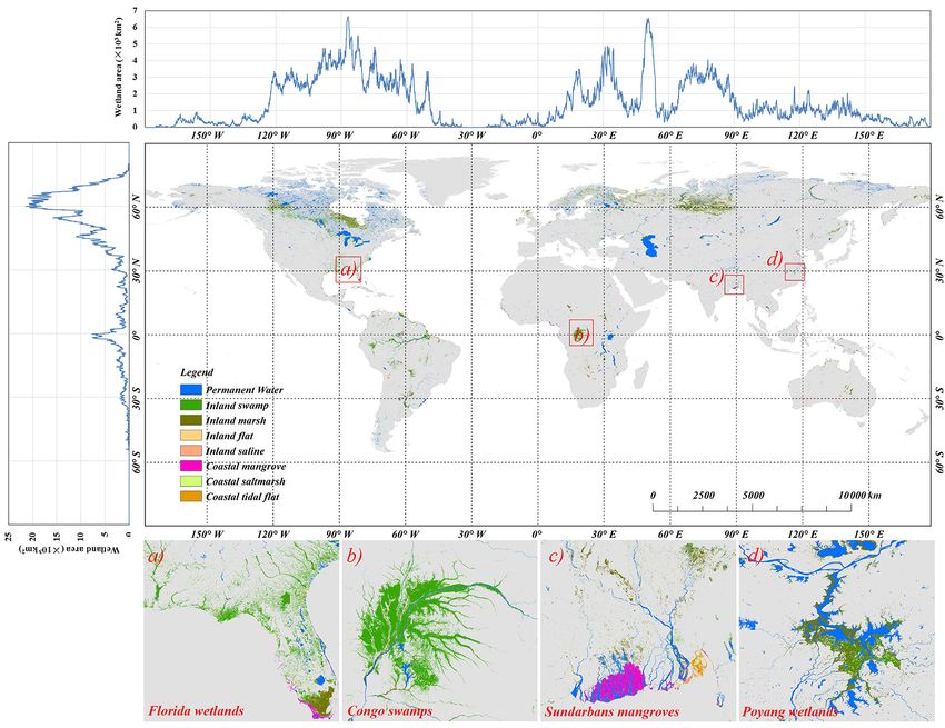
274                                                      X. Zhang et al.: Global 30 m wetland map with fine classification system

Figure 3. The flowchart of wetland mapping using water-level, phenological and topographical features and a stratified classification strategy.

Z. Zhang et al. (2022) found a positive relationship between                 Many studies also demonstrated that a multi-temporal phe-
tidal height and NDWI using field survey data, the maximum                nology was also essential for classifying the vegetated wet-
NDWI compositing was applied to the clear-sky Landsat                     lands and excluding these non-wetland land-cover types (Li
time-series imagery to capture the highest-water-level opti-              et al., 2020; Ludwig et al., 2019). There were usually two op-
cal composites illustrated in Fig. 4b. As for the lowest water-           tions for capturing phenological features from Landsat time-
level features, considering that the tidal and flooded flat or            series imagery. These included seasonal-based compositing
marsh usually reflected higher NDVI and EVI values than                   (Zhang et al., 2021a, 2022) and percentile-based composit-
waterbodies and that Z. Zhang et al. (2022) also used the field           ing (Hansen et al., 2014; Zhang and Roy, 2017; Zhang et
data to demonstrate that there was a negative relationship                al., 2021b). The former used the phenological calendar for
between tidal-level height and NDVI, the maximum NDVI                     selecting time-matched imagery. It then adopted the com-
composite was applied to capture the lowest-water-level op-               positing rule to capture the seasonal features, while the lat-
tical information illustrated in Fig. 4a. Considering that opti-          ter directly used the statistical distributions to select various
cal observations were usually contaminated by clouds, espe-               percentiles. Azzari and Lobell (2017) quantitatively analyzed
cially during the rainy seasons, and that the SAR back coef-              the performance of two compositing methods and found
ficients had a great advantage in the presence of cloud cover-            that both of them had similar mapping accuracy for land-
age and were found to be sensitive to the soil moisture, veg-             cover mapping. Meanwhile, the seasonal-based composit-
etation structure and inundation information, the Sentinel-1              ing method needed the prior phenological calendar, while
SAR time-series imagery could be used as a complemen-                     the percentile compositing method did not require any prior
tary dataset for capturing the highest- and lowest-water-level            knowledge or explicit assumptions regarding the timing of
composites (DeVries et al., 2020; Li et al., 2020; Mahdian-               the season; therefore, the percentile compositing method
pari et al., 2018). Specifically, as the SAR active transmitting          was more suitable for generating phenological features. This
signals were heavily absorbed when they reached the water-                study composited Landsat reflectance time-series bands and
body, the corresponding SAR back coefficients in the water-               four spectral indices into five percentiles (15th, 30th, 50th,
body had lower values compared to other land-cover types.                 70th and 85th) because we wanted to capture as many of
To capture the high-water-level features from the Sentinel-1              the phenological changes in wetlands as possible when com-
time-series imagery, the percentile compositing method us-                paring with the four seasonal composites (Zhang and Roy,
ing the 5th percentile was applied, as illustrated in Fig. 4d.            2017). It should be noted that the minimum and maximum
Conversely, the 95th percentiles of Sentinel-1 VV and VH                  percentiles were excluded because they were usually affected
were generated to capture the lowest-water-level information              by residual clouds, shadows and saturated observations.
(Fig. 4c). It should be noted that the minimum and maxi-                     Lastly, the topographical variables were also important
mum percentiles were not used because the Sentinel-1 time-                factors for determining the spatial distribution of wetlands
series imagery still contained the residual errors caused by              (Ludwig et al., 2019; Tootchi et al., 2019). For example,
the quantitative processing.                                              the widely used topographical wetness index (TWI) uses the
                                                                          local slope to reveal soil wetness, which improves wetland

Earth Syst. Sci. Data, 15, 265–293, 2023                                                     https://doi.org/10.5194/essd-15-265-2023
X. Zhang et al.: Global 30 m wetland map with fine classification system 275
Figure 4. The lowest- and highest-water-level features derived from (a–b) Landsat optical reflectance time-series data and (c–d) the Sentinel-
1 SAR imagery using the time-series compositing method in Poyang Lake, China.
classification performance and reduces commission errors Finally, we spatially mosaicked these 961 regional wetland
within upland areas (Ludwig et al., 2019). Therefore, the ele- maps into the global 30 m wetland map in 2020.
vation, aspect and slope, calculated from the ASTER GDEM Afterward, the random forest (RF) classifier was demon-
dataset, were included in the multi-sourced features. In sum- strated to have obvious advantages, including dealing with
mary, there are a total of 77 multi-sourced training features high-dimensional data, robustness for training noise and fea-
(listed in Table 3), including 70 optical features from Land- ture selection, as well as achieving higher classification when
sat imagery, 4 SAR features from Sentinel-1 imagery and 3 compared to other widely used machine learning classifiers
topographical features from ASTER GDEM. (e.g., support vector machines, neural networks, decision
trees) (Belgiu and Drăguţh, 2016; Gislason et al., 2006).
Therefore, the RF classifier was selected for mapping inland
4.2 The stratified classification strategy for wetland and coastal tidal wetlands using multi-sourced features on the
mapping GEE platform. It should be noted that the RF classifier had
two key parameters: the number of selected prediction vari-
Since we have simultaneously extracted the maximum
ables (Mtry ) and the number of decision trees (Ntree ). Belgiu
coastal and inland wetland extents when deriving training
and Drăguţh (2016) and Z. Zhang et al. (2022) have demon-
samples from prior wetland datasets, the stratified classifi-
strated the quantitative relationship of Ntree against classi-
cation strategy was adopted to fully use the maximum extent
fication accuracy and found that the classification accuracy
constraint. If a pixel was classified as a coastal tidal wetland
stabilized when Ntree was greater than 100. Meanwhile, Bel-
outside the maximum coastal tidal wetland extents, it would
giu and Drăguţh (2016) suggested that Mtry should take its
be identified as a misclassification. Furthermore, there were
default value of the square root of the number of all input
two ideas for the large-area land-cover mapping, including
features. Therefore, Ntree and Mtry took 100 and the square
global classification modeling (using one universal model
root of the number of all input features, respectively.
for entire areas) and local adaptive modeling (using various
The inland and coastal tidal wetland maps were pro-
models for different local zones) (Zhang et al., 2020). For ex-
duced by combining water-level and phenological features,
ample, Zhang and Roy (2017) demonstrated that local adap-
the stratified classification strategy, local adaptive modeling,
tive modeling outperformed the global classification model-
and the derived wetland and non-wetland training samples.
ing strategy. Therefore, the global land surface was first di-
As the inland and coastal tidal wetlands were independently
vided into 961 5◦ × 5◦ geographical tiles illustrated in Fig. 5,
produced, some pixels in the overlapping area of maximum
which were inherited from the global 30 m land-cover map-
inland and coastal tidal wetland extents were simultaneously
ping by Zhang et al. (2021b). Then, we trained the local adap-
labeled as inland wetlands and coastal tidal wetlands. How-
tive classification models using derived training samples in
ever, as the final global wetland map was a hard classifica-
Sect. 3 and multi-sourced and multi-temporal features (the
tion, these pixels should be post-processed into one label.
highest water level, lowest water level, phenological compos-
As the random forest classifier could provide the posterior
ites and topographical variables) at each 5◦ × 5◦ geographi-
probability for each pixel, we determined the labels of the
cal tile. It should be noted that we used the training samples
confused pixels by comparing the posterior probabilities. In
from neighboring 3 × 3 geographical tiles to train the clas-
addition, as the tidal flats were demonstrated to overestimate
sification model and classify the central tile for guarantee-
some coastal ponds as tidal flats, the global lake and reservoir
ing the spatially continuous transition over adjacent regional
dataset, developed by Khandelwal et al. (2022), was applied
wetland maps. Namely, we trained 961 local adaptive classi-
to optimize the tidal flat.
fication models and then produced 961 5◦ ×5◦ wetland maps.
https://doi.org/10.5194/essd-15-265-2023 Earth Syst. Sci. Data, 15, 265–293, 2023276 X. Zhang et al.: Global 30 m wetland map with fine classification system
Table 3. The multi-sourced and multi-temporal training features for wetland mapping.
Data Derived training features from multi-sourced remote
sensing imagery
Water-level features: the lowest and highest com-
Landsat
posites with blue, green, red, NIR, SWIR1, SWIR2,
LSWI, NDWI, NDVI and EVI bands
Phenological features: 15th, 30th, 50th, 70th and
85th percentiles with blue, green, red, NIR, SWIR1,
SWIR2, LSWI, NDWI, NDVI and EVI bands
Sentinel-1 SAR Water-level features: the lowest and highest compos-
ites using 5th and 95th percentiles for VV and VH
bands.
ASTER GDEM Topographical features: elevation, slope and aspect.
Figure 5. The spatial distribution of 961 5◦ × 5◦ geographical tiles used for local adaptive modeling, which was inherited from the global
30 m land-cover mapping by Zhang et al. (2021b). The background imagery came from the National Aeronautics and Space Administration
(https://visibleearth.nasa.gov, last access: 10 November 2022).
4.3 Accuracy assessment where Wi and pi are the area proportion and expected accu-
racy of class i, ni and n are the sample size of class i and total
To quantitatively analyze the performance of our sample size, V is the standard error of the estimated overall
GWL_FCS30 wetland map, a total of 25 709 validation accuracy, and N is the number of pixel units in the study re-
samples (illustrated in Fig. 6), including 10 558 non-wetland gion. Then, as the wetlands had a significant correlation with
points and 15 151 wetland points, were collected. Firstly, as the water levels (Z. Zhang et al., 2022), the time-series op-
the wetland was a sparse land-cover type compared to the tical observations archived on the GEE cloud platform were
non-wetlands (forest, cropland, grassland and bare land), the used as the auxiliary dataset to interpret these water-level-
stratified random strategy was applied to randomly derive sensitive wetlands, such as tidal flat and flooded flat. It should
validation points at each stratum as be noted that the visual interpretation was implemented on
Wi × pi (1 − pi ) the GEE cloud platform because it archives a large number
ni = n × P , of satellite images with various time spans and spatiotempo-
Wi × pi (1 − pi )
ral resolution (X. Zhang et al., 2022). Meanwhile, each val-
P √ 2
Wi pi (1 − pi ) idation point is independently interpreted by five experts for
n= P , (5) minimizing the effect of an expert’s subjective knowledge,
V + Wi pi (1 − pi )/N
Earth Syst. Sci. Data, 15, 265–293, 2023 https://doi.org/10.5194/essd-15-265-2023X. Zhang et al.: Global 30 m wetland map with fine classification system 277
and only these complete agreement points were retained; oth- cause their spectral characteristics quickly changed with the
erwise, they were discarded. Then, we employed four met- seasonal or daily water levels of the underlying surface (Lud-
rics typically used to evaluate accuracy, which include the wig et al., 2019). To quantitatively analyze the importance
kappa coefficient, overall accuracy, user accuracy (measuring of these multi-sourced and multi-temporal features, we used
the commission error) and producer accuracy (measuring the the random forest classification model, which calculated the
omission error) (Gómez et al., 2016; Olofsson et al., 2014), increased mean squared error by permuting the out-of-bag
for calculations using 25 709 global wetland validation sam- data of a variable while keeping the remaining variables con-
ples. stant (Breiman, 2001; Zhang et al., 2020) in an effort to com-
pute their importance. Figure 8 illustrates the importance of
all multi-sourced and phenological features, and it can be
5 Results
found that the phenological features which made the most
5.1 The reliability analysis of derived training samples
significant contribution mainly did so because they used the
multi-temporal percentiles to comprehensively capture vege-
This study proposed combining pre-existing multi-sourced tation phenology (EVI and NDVI) and water-level dynamics
wetland products, refinement rules and expert knowledge to (NDWI and LSWI) for the various land-cover types. Then,
automatically derive these massive inland and coastal tidal the combination of optical and Sentinel-1 SAR water-level
wetland training samples globally. To demonstrate the relia- features was ranked as the second-most-important role in dis-
bility of the derived training samples for wetland mapping, tinguishing the fine wetlands and non-wetlands. Based on
we randomly selected approximately 10 000 points from the the lowest- and highest-water-level features in Fig. 4, the
sample pool and checked their confidence using visual in- highest- and lowest-water-level features greatly contributed
terpretation. It should be noted that we cannot check all the to determining these water-sensitive wetlands (marsh, tidal
training samples because the number of derived samples was flat and flooded flat). For example, Z. Zhang et al. (2022)
massive (exceeding 20 million training samples in Sect. 3). quantitatively analyzed the contribution of multi-sourced
After a point-to-point inspection, these selected training sam- features to mapping accuracy. They found that importing
ples achieved an overall accuracy of 91.53 % in 2020. Mean- water-level features significantly improved the ability to sep-
while, we also used 10 000 selected wetland training samples arate tidal flats from non-wetlands. Lastly, three topograph-
and many non-wetland samples to analyze the overall and ical variables also contributed to wetland mapping because
producer accuracies of coastal and inland wetlands vs. num- the spatial distribution of wetlands had a significant relation-
ber of erroneous training samples. Specifically, we gradually ship with topography and was mainly distributed in low-lying
increased the “contaminated” samples by randomly altering areas (Zhu and Gong, 2014).
the label of a certain percentage of training samples in steps
of 0.01 and then used these “contaminated” samples to build 5.3 The spatial pattern of global wetlands in 2020
the RF classification model. After repeating the process 100
times, the quantitative relationship between mapping accu- Figure 9 illustrates the spatial distributions of our
racies and erroneous samples is illustrated in Fig. 7. Obvi- GWL_FCS30 wetland map and their area statistics in lat-
ously, the overall accuracy and producer accuracy of wet- itudinal and longitudinal directions in 2020. Overall, the
lands (merging seven sub-categories into one wetland) were GWL_FCS30 map accurately captured the spatial patterns
insensitive to the erroneous training samples when the per- of wetlands. It mainly concentrated on the high-latitude areas
centage of erroneous samples was controlled within 20 %. in the Northern Hemisphere and the rainforest areas (Congo
Beyond this threshold, the accuracies slowly decreased along Basin and Amazon rainforest in South America). Quantita-
with the increase in erroneous training samples. Similarly, tively, according to the latitudinal statistics, approximately
previous studies by Zhang et al. (2021b, 2022) quantitatively 72.96 % of wetlands were distributed poleward of 40◦ N (a
analyzed the relationship between overall accuracy and the large number of wetlands are located in Canada and Rus-
erroneous training sample size. They found that the overall sia), and 10.6 % of wetlands were located in equatorial areas,
accuracy stabilized when the percentage of erroneous train- between 10◦ S–10◦ N, within which the Congo and Ama-
ing samples was controlled within the threshold and then zon rainforest wetlands are located. As for the longitudinal
rapidly decreased after exceeding the threshold. Therefore, direction, there were mainly four statistical peak intervals:
the derived training samples in Sect. 3 were accurate enough 120–50◦ W (Canada wetlands and Amazon wetlands), 15–
to support large-area fine wetland mapping. 25◦ E (Congo wetlands), 40–55◦ E (the Caspian Sea) and 60–
90◦ E (Russia wetlands). Afterward, to more intuitively un-
5.2 The importance of multi-sourced phenological
derstand the performance of our GWL_FCS30 wetland map,
features for wetland mapping
four local enlargements in Florida, the Congo Basin, Sun-
darbans and Poyang Lake were also illustrated. All of them
The complicated temporal dynamics and spectral hetero- comprehensively captured the wetland patterns in these lo-
geneity caused great uncertainties in wetland mapping be- cal areas. For example, there was significant consistency be-
https://doi.org/10.5194/essd-15-265-2023 Earth Syst. Sci. Data, 15, 265–293, 2023You can also read