Extreme-coastal-water-level estimation and projection: a comparison of statistical methods - NHESS
←
→
Page content transcription
If your browser does not render page correctly, please read the page content below
Nat. Hazards Earth Syst. Sci., 22, 1109–1128, 2022
https://doi.org/10.5194/nhess-22-1109-2022
© Author(s) 2022. This work is distributed under
the Creative Commons Attribution 4.0 License.

Extreme-coastal-water-level estimation and projection:
a comparison of statistical methods
Maria Francesca Caruso1 and Marco Marani1,2,3
1 Department of Civil, Architectural, and Environmental Engineering, University of Padua, 35131, Padua, Italy
2 Earthand Climate Sciences Division, Duke University, Durham, NC, USA
3 Department of Civil and Environmental Engineering, Duke University, Durham, NC, USA

Correspondence: Maria Francesca Caruso (mariafrancesca.caruso@phd.unipd.it)

Received: 6 August 2021 – Discussion started: 18 August 2021
Revised: 17 February 2022 – Accepted: 23 February 2022 – Published: 1 April 2022

Abstract. Accurate estimates of the probability of extreme        1   Introduction
sea levels are pivotal for assessing risk and for designing
coastal defense structures. This probability is typically esti-
mated by modeling observed sea-level records using one of a       The statistical analysis of extreme values of random variables
few statistical approaches. In this study we comparatively ap-    is of wide conceptual and applicative importance in science
ply the generalized-extreme-value (GEV) distribution, based       and engineering (Coles, 2001; Beirlant et al., 2004; Castillo
on block maxima (BM) and peaks-over-threshold (POT) for-          et al., 2005; Finkenstädt and Rootzén, 2004). Modeling
mulations, and the recent metastatistical extreme-value dis-      extreme-value probability of occurrence is indeed an active
tribution (MEVD) to four long time series of sea-level ob-        field of theoretical and applied research in many fields, such
servations distributed along European coastlines. A cross-        as hydrology and climatology (Katz et al., 2002; Cancelliere,
validation approach, dividing available data into separate cal-   2017; Mekonnen et al., 2021; Miniussi and Marra, 2021),
ibration and test sub-samples, is used to compare their per-      ecology (Katz et al., 2005; Rypkema et al., 2019), ocean
formances in high-quantile estimation. To address the limi-       wave modeling (Rueda et al., 2016; Benetazzo et al., 2017;
tations posed by the length of the observational time series,     Barbariol et al., 2019), transport engineering (Songchitruksa
we quantify the estimation uncertainty associated with dif-       and Tarko, 2006), geophysical processes (Pisarenko et al.,
ferent calibration sample sizes from 5 to 30 years. We study      2014a, b; Elvidge and Angling, 2018; Hosseini et al., 2020),
extreme values of the coastal water level – the sum of the wa-    biomedical data analysis (De Zea Bermudez and Mendes,
ter level setup induced by meteorological forcing and of the      2012; Chiu et al., 2018), insurance and financial applications
astronomical tide – and we find that the MEVD framework           (Embrechts et al., 1997; Chan et al., 2022), and many others.
provides robust quantile estimates, especially when longer           In particular, the reliable estimation of the occurrence
sample sizes of 10–30 years are considered. However, dif-         probability of coastal flooding events of large magnitude is
ferences in performance among the approaches explored are         crucial to environmental hazard evaluation (Coles and Tawn,
subtle, and a definitive conclusion on an optimal solution in-    2005; Hamdi et al., 2018) and to decision-making and mit-
dependent of the return period of interest remains elusive.       igation measure design. In fact, coastal flooding hazard has
Finally, we investigate the influence of end-of-century pro-      been increasing on a global scale in recent decades, a trend
jected mean sea levels on the probability of occurrence of        expected to continue as a result of climate change (Meehl
extreme-total-water-level (the sum of the instantaneous wa-       et al., 2007; Church et al., 2013; Fortunato et al., 2016).
ter level and the increasing mean sea level) frequencies. The     Several studies highlight that global sea-level rise will con-
analyses show that increases in the value of total water levels   tinue accelerating in the 21st century as a consequence of
corresponding to a fixed return period are highly heteroge-       climate change (Church and White, 2006; Jevrejeva et al.,
neous across the locations explored.                              2008; Church and White, 2011; Haigh et al., 2014b; Hay
                                                                  et al., 2015). Additionally, changes in storminess may have

Published by Copernicus Publications on behalf of the European Geosciences Union.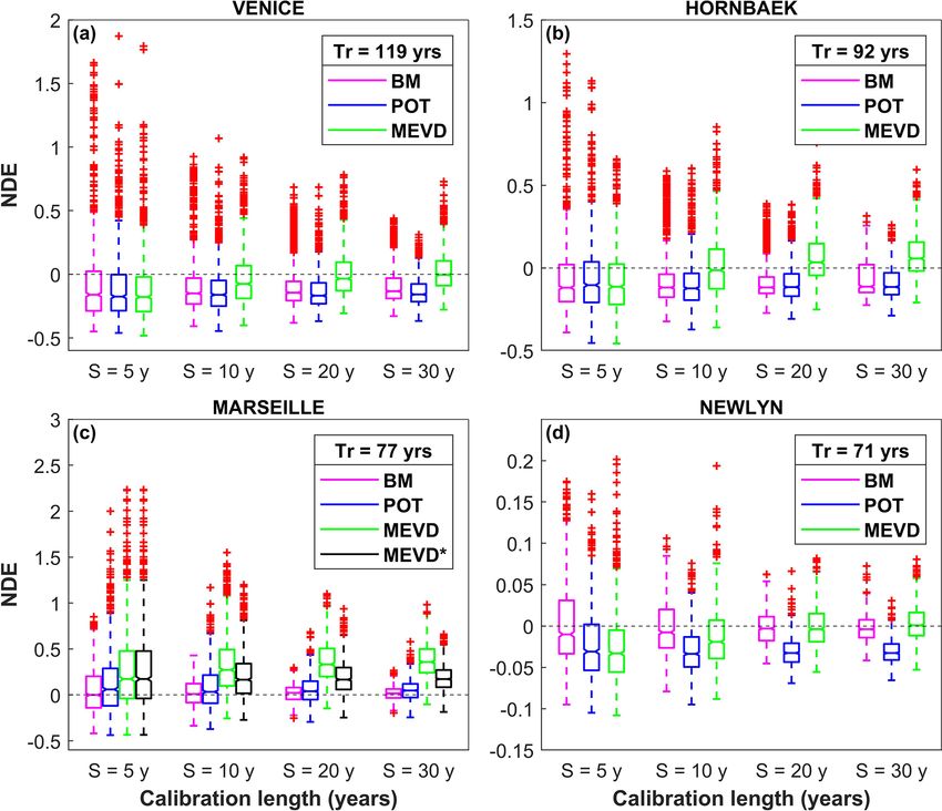
1110                                  M. F. Caruso and M. Marani: Extreme-coastal-water-level estimation and projection

an important role in modifying the frequency and magni-                More generally, GEV-based approaches, by construction,
tude of water level extremes (Lowe et al., 2010; Menéndez           discard most of the observations and do not attempt to op-
and Woodworth, 2010; Woodworth et al., 2011). Much of               timize the use of the available information (Volpi et al.,
the current work on extreme-coastal-flooding events is based        2019). Furthermore, the traditional extreme-value theory de-
on the classical extreme-value theory (EVT) (Fréchet, 1927;         rives the GEV distribution either as the asymptotic distri-
Dalrymple, 1960; Coles, 2001; Woodworth and Blackman,               bution when the number of events per block becomes very
2002; Hamdi et al., 2014, 2015; and references therein),            large or through the ad hoc GPD–Poisson assumptions un-
which identifies the family of distribution functions known as      derlying the POT approach. Whether these hypotheses do
generalized-extreme-value (GEV) distribution (Von Mises,            apply to the case of sea levels is a matter of discussion, but
1936) as a general model for the distribution of maxima (or         it seems beneficial to adopt methods that require the least
minima) extracted from fixed time periods of equal length           number of a priori assumptions on the properties of the event
(“blocks”, most commonly with a length of 1 year). The              arrival process. As a contribution to overcoming the limi-
GEV, according to its original formulation, arises as a lim-        tations of the traditional EVT, here we explore the use of
iting distribution for maxima (or minima, not considered            an alternative approach for modeling extreme sea levels, the
here) of a sequence of independent and identically distributed      metastatistical extreme-value distribution (MEVD). This ap-
(i.i.d.) random variables. The peaks-over-threshold (POT)           proach was introduced by Marani and Ignaccolo (2015) and
formulation (Balkema and de Haan, 1974; Pickands, 1975)             has been previously applied to rainfall, flood-frequency anal-
extends the original GEV derivation by modeling all events          ysis, and hurricane intensities. The MEVD models the distri-
exceeding a high threshold as opposed to considering just           bution of yearly maxima starting from the distribution of “or-
yearly maxima as in the GEV-block maxima formulation                dinary values”, i.e., all the available data, in contrast to just
(GEV–BM). The POT approach again recovers the GEV dis-              considering annual maxima or a few values above a thresh-
tribution as the distribution of the annual maxima if two as-       old. Moreover, the MEVD framework (i) is a non-asymptotic
sumptions are valid (Davison and Smith, 1990): (1) the num-         extreme-value distribution, which does not require the num-
ber of events per year is Poisson-distributed; (2) exceedances      ber of events per year to be large as in the traditional theory,
over the threshold come from a generalized Pareto distribu-         and (ii) makes no a priori assumptions on the properties of
tion (GPD). Under these suitable conditions, in the follow-         the event occurrence process. In previous applications, the
ing we refer to the POT framework as the POT–GPD formu-             MEVD has been shown to significantly reduce estimation
lation. For a brief overview of the theory underlying EVT           uncertainty compared to traditional approaches, especially
and the two main methods based on the GEV distribution              when considering return periods greater than the sample size
(i.e., BM and POT approaches), the reader can refer to the          used for parameter estimation (Zorzetto et al., 2016; Marra
“Methods” section or the Supplement. The POT–GPD ap-                et al., 2018; Miniussi and Marani, 2020; Miniussi et al.,
proach is often considered to be superior to GEV–BM in              2020a, b).
practical applications due to its more efficient use of often          Here we comparatively analyze the performance of GEV-
scarce observations. For extreme-sea-level studies in partic-       based approaches and MEVD in high-quantile estimations
ular, Coles and Tawn (2005) and Haigh et al. (2010) recog-          with application to extreme sea levels at different observa-
nize two weaknesses in the use of the GEV–BM analysis:              tion sites. The aim is to (1) identify the statistical tool afford-
(1) sea level is the combination of tide-driven (deterministic)     ing minimal uncertainty in the estimate of extreme sea levels
and storm-driven (stochastic) components (the presence of           with assigned probability of exceedance and (2) model and
a deterministic component is suggested to violate the i.i.d.        understand how climate change will affect the extreme-sea-
assumption required in the GEV–BM derivation); (2) sea-             level occurrence. To achieve these objectives, we analyze se-
level data are collected frequently (e.g., hourly), while the       lected sea-level time series along the European coastline and
GEV–BM approach only studies annual maxima, with an ex-             evaluate extreme-sea-level predictive uncertainty by adopt-
tremely inefficient use of the data. The POT framework ex-          ing a cross-validation approach in which calibration and test
ploits more of the available information with respect to the        samples are kept separate and independent. Subsequently,
BM approach (e.g., Coles, 2001; Bernardara et al., 2014).           we use the optimized estimation method to infer possible
However, the choice of a suitable threshold to retain a few         changes in coastal flooding hazard under Intergovernmental
above-threshold events per year is a critical step, and the esti-   Panel on Climate Change (IPCC) climate change scenario
mation uncertainty significantly depends on threshold selec-        RCP4.5 and RCP8.5.
tion (Önöz and Bayazit, 2001; Li et al., 2012; Solari et al.,          The structure of the paper is as follows: Sect. 2 outlines the
2017). The selected threshold value implies a balance be-           sea-level data and the methodology used in this application,
tween bias and estimation error variance (Coles, 2001). In          and results are described in Sect. 3, while the conclusions are
fact, too low a threshold will violate the independence hy-         given in Sect. 4.
pothesis of the framework, leading to bias, while too high a
threshold will retain just a few values above the threshold,
leading to high error variance.

Nat. Hazards Earth Syst. Sci., 22, 1109–1128, 2022                                  https://doi.org/10.5194/nhess-22-1109-2022
M. F. Caruso and M. Marani: Extreme-coastal-water-level estimation and projection                                            1111

2     Materials and methods                                        duced tidal level, x(t); and meteorologically induced surge
                                                                   level, y(t):
2.1     Data
                                                                   z(t) = m.s.l.(t) + x(t) + y(t).                             (1)
The analyses were performed using daily and hourly sea-
level records from four tide gauge stations (see Table 1) dis-        The term m.s.l.(t) represents the long-term variations in
tributed along European coastlines: Venice (Italy), Hornbæk        water levels and of the elevation datum (i.e., possible land
(Denmark), Marseille (France), and Newlyn (United King-            subsidence or uplift). Local m.s.l.(t) does not change uni-
dom). The study sites span a variety of geographical loca-         formly over time, and its calculation is affected by many fac-
tions, coastal morphologies, and storm regimes.                    tors, such as tidal phases, long-term wind and atmospheric-
   Venice sea-level data (maximum and minimum                      pressure patterns, and vertical land motion (subsidence or
daily observations) were obtained from the “Centro                 uplift). The tidal contribution to the instantaneous sea level,
Previsioni e Segnalazioni Maree” of the Venice Mu-                 x(t), caused by the gravitational forces exerted by the moon
nicipality         (https://www.comune.venezia.it/it/content/      and the sun is deterministic in nature and can be predicted
centro-previsioni-e-segnalazioni-maree, Città di Venezia,          with a good degree of accuracy. This tidal variability oc-
2020) for the Punta della Salute gauge station. The remain-        curs with characteristic periodicities between 12 h and 18.61
ing water level data, all at the hourly scale, were downloaded     years (Eliot, 2010; Haigh et al., 2011; Pugh and Woodworth,
from the University of Hawaii Sea Level Center (UHSLC)             2014; Peng et al., 2019; Valle-Levinson et al., 2021). This lat-
repository (http://uhslc.soest.hawaii.edu/data/?rq#uh745a/,        ter longest tidal periodicity corresponds to the precession of
last access: 10 November 2020; Caldwell et al., 2015).             the lunar nodal cycle. The storm-surge contribution, y(t), is
   All sea-level datasets span long observational periods: 148     the meteorologically induced change in the water level gen-
years for Venice, 122 years for Hornbæk, 115 years for Mar-        erated by a combination of factors, such as the magnitude
seille (ca. 19 missing years), and 102 years for Newlyn.           and direction of the wind, spatial gradients in atmospheric
   The raw data for all stations were pre-processed to elim-       pressure, storm size, fetch, bathymetry, and storm duration
inate (1) years with less than 6 months of water level ob-         (Hall and Sobel, 2013).
servations and (2) days with less than 24 h of data (for the          Two classes of methods are widely used to estimate the
case of hourly data). This process yields four “cleaned up”        probability of occurrence of extreme sea levels: direct and
time series that were subsequently used in the analyses (see       indirect methods. Indirect methods model separately the
Table 1). Figure 1 shows daily maximum sea levels at the           deterministic and the stochastic components of z(t), fol-
gauge stations explored after pre-processing.                      lowed by a convolution to obtain the probability distribu-
                                                                   tion of their sum. Examples are the joint probability method
                                                                   (Pugh and Vassie, 1978, 1980), the revised joint probabil-
2.2     Methods                                                    ity method (Tawn and Vassie, 1989), the exceedance proba-
                                                                   bility method (Middleton and Thompson, 1986; Hamon and
2.2.1    Mean-sea-level removal                                    Middleton, 1989), and the empirical simulation technique
                                                                   (Scheffner et al., 1996; Goring et al., 2011). Direct meth-
                                                                   ods, such as the one adopted here, analyze observed values
The sea-level sequence is highly correlated and is generated
                                                                   compounding the astronomical and stochastic storm-surge
by a non-stationary process due to long-term trends in mean
                                                                   component. Direct methods mostly differ based on the anal-
sea level, the deterministic tidal component, surge seasonal-
                                                                   ysis approach adopted, such as the annual maxima method
ity, and interactions between the tide and surge (Dixon and
                                                                   (Jenkinson, 1955; Gumbel, 1958), the peaks-over-threshold
Tawn, 1999). Tide–surge interactions may change amplitude
                                                                   method (Davison and Smith, 1990), or the r-largest method
and phase of the surges, mostly in shallow estuarine areas
                                                                   (Smith, 1986; Tawn, 1988). Here, we study the distribution
(Johns and Ali, 1980; Bernier and Thompson, 2007; Zhang
                                                                   of the sum, h(t), of the contributions from the deterministic
et al., 2010). Therefore, this effect needs to be taken into ac-
                                                                   tide and the stochastic surge:
count when separating the surge and tide components. How-
ever, here, we do not attempt to separate these contributions;     h(t) = z(t) − m.s.l.(t).                                    (2)
we only analyze the sum given by the combination of the wa-
ter level setup, induced by meteorological forcing, and the           From a statistical point of view, this choice is justified by
astronomical tide. Hence, we simply study such sum as the          the fact that the random arrival of storms adds a stochas-
final result of the nonlinear interactions between individual      tic surge contribution at unpredictable times, thereby caus-
components. Under this premise, for a given site and at any        ing h(t) to be values from a random variable, even though
instant of time t, the observed sea level z(t) (after averag-      it contains a deterministic component. The presence of a de-
ing out waves) can be split into three components (Pugh and        terministic component of course does imply a strong auto-
Vassie, 1978): mean sea level, m.s.l.(t); astronomically in-       correlation in the observed signal, which will be subse-

https://doi.org/10.5194/nhess-22-1109-2022                                Nat. Hazards Earth Syst. Sci., 22, 1109–1128, 2022
1112                                     M. F. Caruso and M. Marani: Extreme-coastal-water-level estimation and projection

Table 1. Information of sea-level data used in this application.

                                           Location (degree, minutes)                    Missing        Deleted   Number
                Site name     Country                                         Period
                                                   Lat             Long                years (%)          years   of years
                Venice        Italy        45◦ 25.0’ N      12◦ 20.0’ E   1872–2019            –              –       148
                Hornbæk       Denmark      56◦ 06.0’ N      12◦ 28.0’ E   1891–2012            –          1985        121
                                                                                                    1897, 1918,
                                                                                                    1919, 1928,
                Marseille     France       43◦ 16.7’ N       5◦ 21.2’ E   1885–2018         14.2                      106
                                                                                                    1937, 1940,
                                                                                                    1998, 2009,
                                                                                                           2010
                              United
                Newlyn                     50◦ 06.1’ N      5◦ 32.5’ W    1915–2016            –    1984, 2010        100
                              Kingdom

Figure 1. Daily maximum sea levels at different gauge stations explored after pre-processing: Venice (IT), Hornbæk (DK), Marseille (FR),
and Newlyn (UK).

quently filtered out by suitable signal processing described              ses of (i) the study of long-term trends of maximum yearly
below.                                                                    departures from the average mean sea level (two-tail Mann–
   Here, m.s.l.(t) is computed as the yearly average of daily             Kendall test; Mann, 1945) and (ii) statistical inference of past
levels. The yearly average is chosen rather than the custom-              coastal flooding events and their potential future changes.
ary 19-year average that eliminates all tidal periodicities,                 In the following discussion, we use the terms “total water
however small in amplitude, to better capture the surge con-              level” and “coastal water level” when referring to the quanti-
tribution that causes the water level to deviate during a storm           ties z(t) and h(t), respectively.
with respect to the “current” yearly value of m.s.l.(t). Once
h(t) is computed by removing m.s.l.(t) from recorded levels,
all local maxima of h(t) or water level peaks are identified,
and their values constitute the basis for subsequent analy-

Nat. Hazards Earth Syst. Sci., 22, 1109–1128, 2022                                       https://doi.org/10.5194/nhess-22-1109-2022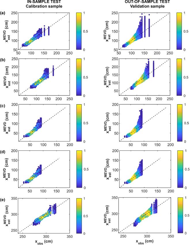
M. F. Caruso and M. Marani: Extreme-coastal-water-level estimation and projection                                             1113

2.2.2   Extreme-value theory                                        the excesses are uniquely determined by those of the asso-
                                                                    ciated GEV distribution of block maxima (see, e.g., Coles,
As highlighted by Serinaldi and Kilsby (2014), the EVT              2001). In particular, the shape parameter, ξ , is equal to that
deals with the asymptotic distributional behavior of two            of the corresponding GEV distribution, and the scale parame-
types of data modeled with two well-known approaches,               ters of the two distributions are related by σu = σ +ξ ·(u−y).
namely the so-called block maxima (BM) and peaks-over-                 The interested reader can refer to Coles (2001) for a de-
threshold (POT) approaches. The first type models the max-          tailed description of statistical methods for extremes in hy-
imum values extracted from blocks of fixed length, whereas          drology or Papalexiou and Koutsoyiannis (2013) for a recent
the second one models all the exceedances of high thresh-           overview of the history of the EVT.
old. The cornerstones of the EVT are two theorems: the
Fisher–Tippett–Gnedenko theorem (also known as the three-           2.2.3   The metastatistical extreme-value distribution
types theorem; Fisher and Tippett, 1928; Gnedenko, 1943;
Gumbel, 1958) and the Pickands–Balkema–de Haan theo-                The typical EVT derivation starts from the premise that the
rem (also known as the second theorem of EVT; Balkema               maximum value among n realizations of a random variable
and de Haan, 1974; Pickands, 1975).                                 (Mn ) is distributed according to the cumulative distribution
   According to the three type theorem, there are three possi-      function P (Mn ≤ x) = G(x) = F (x; θ)n (where, as custom-
ble non-degenerate distribution functions which can arise as        ary, a capital letter indicates the random variable, and a
limiting distributions of extremes of random samples: (i) the       lower-case letter indicates a value of the random variable).
Gumbel distribution, or type I; (ii) the Fréchet distribution, or   This approach assumes that the n values of the random vari-
type II; and (iii) the reverse-Weibull distribution, or type III.   able of interest are generated by the same distribution, the
The above three limiting distribution laws can be combined          “ordinary value” distribution F (x; θ ), and are thus indepen-
into a single family of three-parameter distribution known as       dent and identically distributed; n is the number of events
the generalized-extreme-value (GEV) distribution given by           in a block, such that G(x) is the cumulative distribution of
                                                                    the block maxima. The classical EVT assumes either that
                              ξ                                     the number of events per block is large (asymptotic hypothe-
G(x; µ, ψ, ξ ) = exp{−[1 +      · (x − µ)]}−1/ξ ,            (3)
                              ψ                                     sis, leading to the GEV–BM formulation) or that the number
                                                                    of events per block above a high threshold is distributed ac-
                                            ξ                       cording to a Poisson distribution (POT–GPD formulation).
defined in the region for which {x : 1 +      · (x − µ) > 0}. In
                                            ψ                       The recently proposed metastatistical extreme-value distri-
Eq. (3) µ ∈ (−∞, +∞) is a location parameter, ψ > 0 is a            bution (Marani and Ignaccolo, 2015) is a doubly stochastic
scale parameter, and ξ ∈ (−∞, +∞) is a shape parameter              approach (Dubey, 1968; Beck and Cohen, 2003) that relaxes
which controls the nature of the tail distribution (Fréchet type    these hypotheses by considering both the parameters (θ ) of
for ξ > 0, Gumbel type for ξ = 0, and reverse-Weibull type          the ordinary value probability distribution and the number of
for ξ < 0).                                                         events per block to be random variables. Hence, the MEVD
    The second theorem of EVT defines a method to model the         cumulative distribution of block maxima (estimated using a
tail of the distribution above a threshold value (Davison and       much greater sample than just yearly maxima used in the BM
Smith, 1990). In particular, the theorem states that for a large    approach) is then defined as the compound probability:
enough threshold value, u, the distribution of exceedances of
some high threshold (y = X − u, where X is a sequence of                     +∞ Z
                                                                             X
i.i.d. random variables) is described by a generalized Pareto       G(x) =              F (x; θ )n g(n, θ )dθ ,                 (5)
                                                                             n=1
distribution (GPD), which has the following cumulative dis-                        2
tribution function:
                                                                    where g(n, θ ) is the joint probability distribution of the num-
                         ξ                                          ber of events in a block and of the parameter vector (discrete
G(y; σu , ξ ) = 1 − (1 +    · y)−1/ξ ,                       (4)
                         σu                                         in N and continuous in 2), and 2 is the population of all
                                                                    possible parameter values.
defined on {y : y > 0 and (1 + σξu · y > 0)}, where σu and ξ           For practical applications, the MEVD can be approxi-
are the scale and shape parameters, respectively.                   mated by substituting the ensemble average in Eq. (5) with
There is a link between these two distributions according to        the sample average computed over all the blocks in the time
which, if block maxima have approximate GEV distribution,           series, obtaining
then threshold excesses have corresponding approximate dis-
                                                                                M
tribution within the generalized Pareto family and vice versa,               1 X
                                                                    G(x) ∼
                                                                         =          F (x; θj )nj ,                              (6)
and GEV can be obtained from GPD under two appropriate                       M j =1
conditions (i.e., the occurrences are Poisson-distributed, and
excesses over the threshold come from a GPD). The duality           where M is the number of blocks in the historical record,
between Eqs. (3) and (4) means that the GPD parameters of           F (x; θ j ) is the cumulative distribution of ordinary values in

https://doi.org/10.5194/nhess-22-1109-2022                                  Nat. Hazards Earth Syst. Sci., 22, 1109–1128, 2022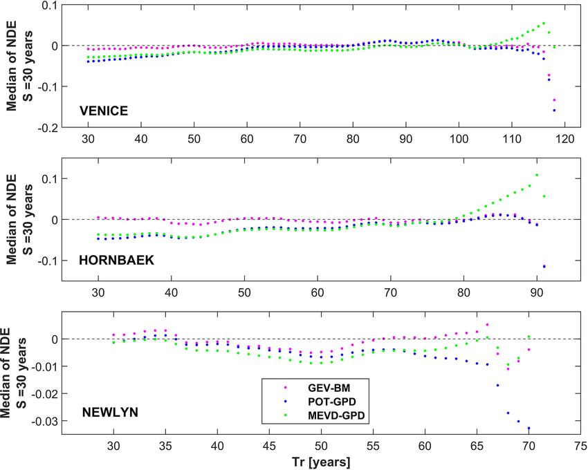
1114                                  M. F. Caruso and M. Marani: Extreme-coastal-water-level estimation and projection

the j th block, and nj is the number of events in the j th block.   straints, we also choose the threshold value that minimizes
A common choice for the block length is 1 year. Note that           the estimation error under the MEVD framework.
the values of the parameter θ j may be estimated on an es-             As suggested by several rainfall applications, ordinary dis-
timation window (EW) with a length that is different from           tribution parameters are here estimated using the probability-
block length. For example, if the block length is 1 year, it        weighted moments (PWMs) method in non-overlapping es-
may be advantageous to estimate parameter values on longer          timation windows of 5 years. In the present application, the
time slices to ensure, depending on the rate of event occur-        optimal estimation window length was set to 5 years to obtain
rence, that a reliable estimation of the parameters is possible.    a more robust parameter estimation, especially when few val-
Miniussi and Marani (2020) in applications to daily rainfall        ues in each year are available. PWM estimation, introduced
extremes find that, when the number of events per year is           by Greenwood et al. (1979), is widely applied because of
fewer than 20–25, then the optimal EW length may be greater         its good performance, particularly in the presence of small
than 1 year.                                                        sample sizes, and its reduced estimation bias and sensitivity
   It is interesting to note that the POT approach, briefly         to the presence of outliers in the data (Hosking et al., 1985;
described above, can be thought of as a particular case             Hosking and Wallis, 1987; Hosking, 1990).
of MEVD. In fact, Zorzetto et al. (2016) highlight that if
one assumes (i) x to be the excess over a high threshold,           2.2.4   Selection of independent events
(ii) F (x; θ j ) to be a generalized Pareto distribution (with
fixed, deterministic parameters), and (iii) n to be generated       The GEV-based approaches are fit on either annual peak
by a Poisson distribution, then the GEV distribution is recov-      maxima (GEV–BM) or on a few water level peaks over a
ered as a particular case of the MEVD by means of the POT           high threshold (POT–GPD), which can be assumed to be re-
approach.                                                           alizations of independent stochastic variables. The MEVD
   MEVD has been applied in several earth-science con-              requires that all ordinary values (coastal-water-level peaks in
texts. In rainfall extreme estimates, the ordinary value dis-       this case) within one block may be assumed to be realizations
tribution is assumed to be Weibull when applied to point            from independent random variables. This hypothesis, in turn,
daily rainfall (Marani and Ignaccolo, 2015; Zorzetto et al.,        requires that observed peaks are filtered to only retain events
2016; Schellander et al., 2019; Miniussi and Marani, 2020;          that may be considered to be independent, through a declus-
Miniussi et al., 2020b), point sub-daily rainfall (Marra et al.,    tering process (Coles, 2001; Ferro and Segers, 2003; Beirlant
2018), and satellite rainfall estimates (Zorzetto and Marani,       et al., 2004; Bommier, 2014; Marra et al., 2018). Several cri-
2019, 2020). For floods across the United States, Miniussi          teria have been developed for such processing of the data.
et al. (2020a) propose to adopt a gamma distribution for            A common criterion sets the minimal time separation, or lag
F (x; θ j ). Hosseini et al. (2020) describe Atlantic hurricane     (τ ), for two events to be considered independent. Intuitively,
intensities using a generalized Pareto ordinary value distribu-     high-water-level events separated by a sufficiently long time
tion. In all cases the appropriate form for the underlying ordi-    period are reasonably caused by distinct storm events. How-
nary value distribution was identified by minimizing the esti-      ever, when analyzing the water level with respect to current
mation uncertainty within a cross-validation approach, which        mean sea level, a quantity that contains the deterministic tidal
is also followed here. In this particular application to extreme    contribution, dependence may be expected to be present also
coastal water levels, three candidate probability distributions     for large lags. In theory, some dependence is present for lags
for F (x; θ j ) in Eq. (6) are tested, i.e., the gamma, Weibull,    up to the longest periodicity in the tidal signal (18.61 years).
and generalized Pareto distributions. Based on the compar-          In practice, as the dependence in the tidal signal decreases
ative evaluation of the performance of these distributions,         for increasing lag, one expects that a much shorter threshold
e.g., using diagnostic quantile–quantile scatterplots, the gen-     time lag will be sufficient to make sure that only independent
eralized Pareto distribution emerged as the best model for the      events are considered. The analysis of the correlograms of se-
“ordinary” coastal-water-level values.                              lected coastal-water-level peaks shows that some correlation
   In the present context, we define as ordinary values             persists also for long time lags and also in the declustered
any coastal water elevation (i.e., the maximum water level          time series. Even though the strength of this correlation is
reached during a storm event) greater than a site-specific          relatively small (the autocorrelation function, ACF, is always
threshold value. This threshold is chosen to be as small as         less than 0.3), it could impact the ability of the MEVD, which
possible (differently from the POT approach) to retain as           assumes independence, to capture observed extreme behav-
much of the observational information as possible and will          ior. The declustering process does significantly decrease cor-
be dependent on the magnitude of the local tidal range (sea-        relation, as may be seen by comparing Fig. S1 (ACF prior to
level difference between high and low water level over a tidal      declustering) and Fig. S2 (after declustering). Interestingly, it
cycle) and of storm contributions. Additionally, the thresh-        is seen that the tidal contribution (that generates periodicities
old is set to be large enough to filter out coastal-water-level     in the ACF) is strongly visible in Venice and Newlyn, while
peaks that are likely fully determined by tidal fluctuation in      it is quite small in Hornbæk and Marseille. The underlying
the absence of any storm contribution. Given the above con-         tidally induced correlation becomes more clearly visible after

Nat. Hazards Earth Syst. Sci., 22, 1109–1128, 2022                                  https://doi.org/10.5194/nhess-22-1109-2022
M. F. Caruso and M. Marani: Extreme-coastal-water-level estimation and projection                                               1115

declustering also in Hornbæk and Marseille. We note that the       distribution in each year and the distribution of the number
existing literature implementing declustering approaches to        of events per year and (2) remove possible non-stationarity
coastal level signals normally focuses on studying the storm-      and correlation in the time series; (b) we divide the ob-
surge component only. As a result, it uses threshold time lag      servational sample into two independent sub-samples ob-
values that are smaller than those adopted here because char-      tained by randomly selecting S years from the original
acteristic correlation times of the surge component are signif-    time series of length M; this sub-sample (in the follow-
icantly smaller than those associated with the sum given by        ing “calibration sample”) is used for parameter estimation,
the combination of surge and tidal components. For exam-           while data in the remaining V = M − S years are used
ple, the independence between two consecutive storm surge          for testing (in the following “validation sample” or “test
events in southern Europe has been found to be achieved            sample”); (c) as usual in frequency analysis, we associate
with a threshold lag of 3 d (Cid et al., 2015). A threshold        with each observed yearly maximum, xi , an empirical fre-
separation of 1 d between consecutive events is imposed by         quency value given by Weibull’s estimator Fi = i/(V + 1),
Tebaldi et al. (2012) in their analysis of storm surges along      where i is the rank of xi in the list of yearly maxima
the US coast. Haigh et al. (2010) adopt a threshold lag of         sorted in ascending order, and V = M − S is the sample
30 h in the English Channel, while Bernardara et al. (2011)        size in the validation sub-sample; the return period Tr as-
assume a 72 h independence criterion. After exploring val-         sociated with each yearly maximum is then simply Tr,i =
ues between 24 h and several days, we adopt a threshold lag        1/(1 − Fi ); (d) we estimate the GEV and MEVD quantiles
of 30 d, which yielded the minimum estimation error under          using the parameter values estimated in step (b) from the
the MEVD approach and is consistent with the main lunar            calibration sub-sample; (e) focusing on the validation sub-
periodicity. The result of this declustering process is a set of   sample, in every realization (for p = 1, . . ., Nr ; Nr = 1000
independent events with magnitudes hk , whose number nj in         here) and for a fixed mean recurrence time (Tr ), we com-
year – or block – j is a realization of a random variable as       pute the nondimensional error (NDE) between the estimated
illustrated in Eqs. (5) and (6).                                   and observed quantiles as NDEp (S, Tr ) = [h(est, p) (S, Tr ) −
                                                                   h(obs, p) (S, Tr )]/h(obs, p) (S, Tr ); (f) we repeat the CV scheme
2.2.5   Cross-validation procedure                                 above Nr times. This procedure is performed for different
                                                                   calibration sample sizes (S = 5, 10, 20, and 30 years) to eval-
Statistical modeling aims to use sample information to infer       uate how estimation uncertainty varies with return period and
the probability distribution of the population from which the      calibration sample size.
data are extracted. This inference is uncertain due to imper-
fect parameter estimates and to the possible inability of the      2.2.6   Future total water level projections
chosen distribution to capture the statistical properties of the
underlying population. Although these sources of uncertainty       Future increases in the frequency of extreme total water lev-
are inherent in any statistical model, their impact can be min-    els (i.e., the variable previously referred as z(t)) due to cli-
imized by a careful choice of the model and by an effective        mate change will have serious impacts on coastal regions.
use of all sources of information (Coles, 2001). In many ap-       These impacts will vary temporally and regionally, depend-
plications uncertainty is estimated by means of goodness-of-       ing on (i) the local relative mean-sea-level rise (including
fit measures, which quantify how well the distribution com-        possible subsidence or uplift), (ii) current storm-surge inten-
pares to the sample on which it was fitted. However, this          sity probability distributions, and (iii) changes in the domi-
procedure does not provide a measure of the predictive un-         nant meteorological dynamics. In this particular application
certainty encountered when trying to estimate the probabil-        to extreme coastal water levels (i.e., the sum given by the
ity of occurrence of the “next” yet unobserved value. In this      combination of the water level setup, induced by meteoro-
study, we evaluate the performance in high-quantile estima-        logical forcing, and the astronomical tide), only the first two
tion associated with the use of the MEVD and the GEV dis-          factors are considered.
tribution by means of a cross-validation (CV) procedure, in           It is very likely that sea-level rise will continue to acceler-
which model predictions of the probability of occurrence are       ate over time, thereby increasing the frequency of extreme-
compared to frequencies from data that were not used in the        sea-level events, leading to severe flooding in many low-
estimation of model parameters. This is possible by dividing       lying coastal cities and small islands (Oppenheimer et al.,
observations into two sets of independent data: the estimation     2019). Various techniques have been used to study possi-
set is the sample from which model parameters are estimated,       ble changes in coastal flooding hazard (e.g., McInnes et al.,
and the test set is the sample with which model predictions        2013; Vousdoukas et al., 2016). Several authors have found
are compared.                                                      that past variations in the frequency of occurrence of ex-
    The procedure can be summarized as follows: (a) we             treme sea levels have been primarily determined by changes
randomly reshuffle the observational years on record while         in mean sea level (e.g., Zhang et al., 2000; Woodworth and
keeping all the independent water level peaks in their orig-       Blackman, 2004; Lowe et al., 2010; Menéndez and Wood-
inal year to (1) preserve both the ordinary value frequency        worth, 2010; Haigh et al., 2014b; Wahl et al., 2017). This

https://doi.org/10.5194/nhess-22-1109-2022                                 Nat. Hazards Earth Syst. Sci., 22, 1109–1128, 2022
1116 M. F. Caruso and M. Marani: Extreme-coastal-water-level estimation and projection
implies that effects of variations in storminess (e.g., magni- Therefore, the return period of the level value h is the in-
tude, trajectories, and frequency) have been small in the ob- verse of the probability of exceedance and can be expressed
servational record compared to the dominant effects of mean- as a function of the cumulative distribution, G(h), of annual
sea-level changes (Haigh et al., 2014a). This notion is also maxima, e.g., through the MEVD (Eq. 6):
confirmed by our trend analyses of maximum yearly depar-
tures from the average sea level (see Sect. 3.1), which fail to 1 1
Tr (h) = = . (7)
detect trends in the maximum difference between total sea E(h) 1 − G(h)
level and concurrent mean sea level except at one of the sites
(Venice), where it is smaller (0.7 mm yr−1 ) than past and pro- Because for a fixed value of mean sea level there is a one-to-
jected rates of sea-level rise (∼ 3.0 and ∼ 8.0 mm yr−1 , re- one relation between the value of the sum of the astronomical
spectively, by the end of the century, according to the RCP8.5 and the storm surge contribution, h, and the total water level,
IPCC scenario). z = h + m.s.l., one can write Gh (h) = P [H > h] = P [H >
Based on these elements, here we estimate the probability z−m.s.l.] = P [Z−m.s.l. > z−m.s.l.] = P [Z > z] = Gz (h)
of future total water levels along European coastlines by as- such that Eq. (7) can be used once the cumulative distribution
suming that changes in the tidal and storm-surge components is known and for each (time-dependent) value of m.s.l. to
are negligible with respect to changes in mean sea level, determine the return period of the total water level (at the
an assumption common to previous approaches (Araújo and time when m.s.l. is evaluated):
Pugh, 2008; Haigh et al., 2010; Tebaldi et al., 2012). 1 1 1
To assess how the exceedance probabilities of extreme Tr (z) = = = . (8)
1 − Gz (h) 1 − Gh (h) 1 − G(z − m.s.l.)
total water levels might change in the future, the pro-
jections of sea-level rise through 2100 from the IPCC’s Based on the hypothesis introduced in Sect. 2.2.6 that mean-
Fifth Assessment Report (AR5) are used. In particular, sea-level rise is the dominant effect in future coastal flooding,
we explore an intermediate (RCP4.5) and an extreme sce- we assume that the characteristics of the extremes (i.e., the
nario (RCP8.5), using CMIP5 model outputs from the “In- parameters of the GPDs defining the MEVD) remain valid
tegrated Climate Data Center” (ICDC) database (Univer- in future scenarios. Equation (8) clarifies that the return pe-
sity of Hamburg: https://icdc.cen.uni-hamburg.de/en/ar5-slr. riod of a fixed value z decreases as m.s.l. increases, basically
html, Church et al., 2013). because for higher values of m.s.l. a smaller value of h is
For each tide gauge, our approach can be summarized needed to achieve the same total water level z. This decrease
as follows: (1) we infer the probability distribution of ex- is nonlinear due to the nonlinear form of the right-hand side
treme coastal water levels (annual maxima) from observed in Eq. (8).
independent events whose intensity (maximum coastal water
level attained, hk ) is defined with respect to the concurrent
mean sea level computed on a yearly basis; (2) we estimate 3 Results and discussion
the future probability of extreme total water levels by trans-
lating extreme-level quantile estimates upward according to 3.1 Mann–Kendall trend analysis
location-specific projections of mean sea level in the year
2100 (thereby implicitly assuming subsidence and uplift to We start by computing mean sea level on a yearly basis and
be negligible). by subtracting it from observed total water level. The first
question that we want to explore is the presence of long-term
2.2.7 Return period trends, unrelated to sea-level rise and associated with other
factors (e.g., human-induced factors, morphological varia-
One of the main objectives of frequency analysis is to cal- tions), in the “cleaned up” signal, i.e., the observed measure-
culate the average recurrence interval or return period. It is ments without mean sea level. To answer this question, in
a widely used concept in hydrological and geophysical risk this work we focus on the deviation of yearly maxima from
analysis. If a process is stationary, the return period (Tr ) of an yearly mean sea level and test for the presence of a trend by
event magnitude is defined as the average time elapsing be- the two-tail Mann–Kendall test (Mann, 1945). Figure 2 sum-
tween two consecutive exceedances of this magnitude. Alter- marizes results for each location explored. From a first vi-
natively, it may be said that a magnitude value is expected to sual inspection of Fig. 2, the Venice (1872–2019) and Horn-
be exceeded, on average, in each return period. If the yearly bæk (1891–2012) time series appear to show an increasing
maximum magnitude h is exceeded on average once in Tr trend in the deviations of yearly maxima from yearly mean
years, then its exceedance probability, E(h) = 1 − G(h), in a sea level (blue line) of different magnitudes. In contrast, Mar-
given year is seille sea-level observations (1985–2018) seem to be charac-
terized by a decreasing trend. Finally, the Newlyn historical
1 record (1915–2016) displays a fairly constant signal with no
E(h) = P [H ≥ h] = . noticeable variations. The application of the Mann–Kendall
Tr (h)
Nat. Hazards Earth Syst. Sci., 22, 1109–1128, 2022 https://doi.org/10.5194/nhess-22-1109-2022M. F. Caruso and M. Marani: Extreme-coastal-water-level estimation and projection 1117
test reveals a partly different story. The test rejects the hy- ple of ordinary values is chosen by testing different threshold
pothesis of the absence of a trend at the 95 % confidence values and evaluating the goodness of fit of the distribution
level only for the Venice site (p valueVenice = 0.014). This using diagnostic graphical plots. According to the selection
result suggests that the increase in the yearly maximum de- criteria described in Sect. 2.2.3, the low thresholds adopted at
viations from yearly mean sea level may be a direct result of the four study sites are 59 cm for Venice, 40 cm for Hornbæk,
the local morphological variations in lagoon channels where 25 cm for Marseille, and 250 cm for Newlyn. For every ob-
the tidal wave propagates (whereby dissipation of the wave served site, Table 2 and Fig. S3 display the gradual increase
is reduced) and/or land subsidence. In contrast, at the re- in the number of independent events (i.e., annual maxima,
maining locations, the null hypothesis of no trend cannot exceedances over the threshold, and ordinary values) used
be rejected (p valueHornbæk = 0.352, p valueMarseille = 0.110, to infer the distributions when moving from GEV–BM and
and p valueNewlyn = 0.997). The results obtained from these POT–GPD to MEVD approaches.
analyses support the validity of the hypothesis that mean- Considering the above threshold values, the observed and
sea-level rise is the dominant factor in determining the future estimated distributions of coastal water level are compared
frequency of coastal flooding (see Sect. 2.2.6). For the tests by plotting their quantiles against each other. By compar-
performed here to compare different extreme-value statisti- ing measures of in-sample and out-of-sample test predictive
cal models, the possible presence of trends (e.g., in Venice) accuracy, the results are presented by means of quantile–
is irrelevant since such tests are performed by first reshuf- quantile (QQ) plots. The reader can refer to Fig. 3 (or
fling observed values, thereby eliminating any existing trend, Figs. S4, S5, S6, S7, and S8 in the Supplement) to com-
albeit small. pare the results obtained with the MEVD framework (or the
GEV-based approaches – GEV–BM and POT–GPD – vs. the
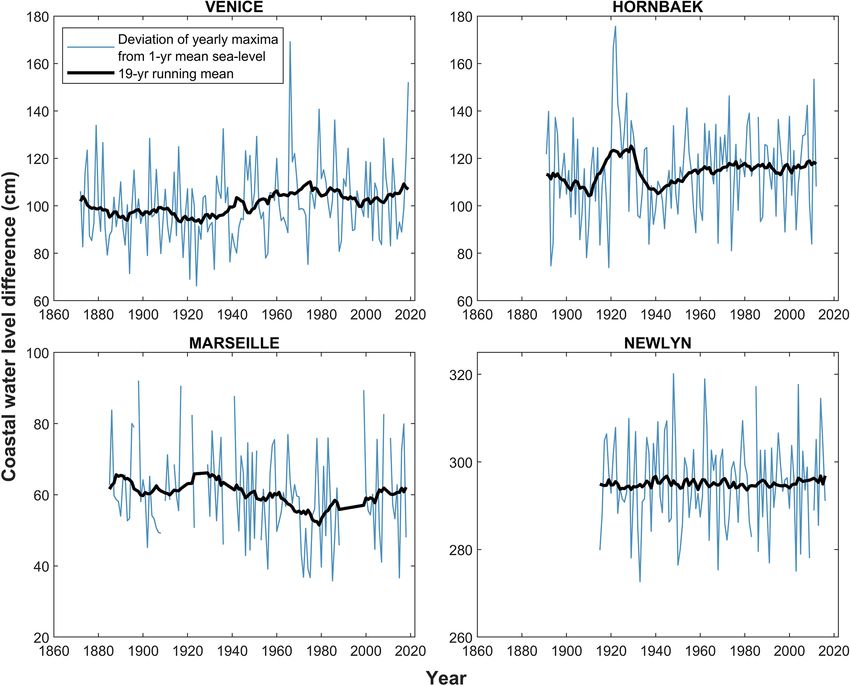
3.2 Extreme-value analysis MEVD formulation) for the four sites analyzed. QQ plots are
obtained as a result of the CV procedure with 1000 random
The MEVD formulation requires the choice of an optimal realizations and sample size: (a) S = 30 years (in-sample
distribution of ordinary values that can represent the charac- test in the left column), (b) V = M − S years (out-of-sample
teristics of the natural phenomenon under analysis. Different test in the right column). The colors represent the density of
candidate distributions for the F (x; θ j ) in Eq. (6) are eval- points around the 45◦ line (i.e., the line of equality). This
uated, and the most suitable distribution is selected on the highlights how the estimated quantiles are closely compara-
basis of the CV procedure comparing the MEVD-estimated ble with the observed ones for all the three approaches tested
quantiles with the observed ones. As previously introduced in and for both the sample sizes explored (S and V ). In particu-
Sect. 2.2.3, according to different tests, the appropriate distri- lar, if the reader looks at Figs. S4–S8 in the Supplement and
bution to model the ordinary sea-level values is the general- if out-of-sample performance is considered, it is difficult to
ized Pareto distribution (GPD). We highlight that the GPD quantify which distribution is the best due to a large variabil-
used in the MEVD framework is obtained by imposing a ity in the estimates. Overall, if only the MEVD performance
small threshold (differently from the high threshold adopted is investigated, the reader can look to the right column (out-
in the POT–GPD approach) to capture the distribution of of-sample test) in Fig. 3, where the results display that the
the main body of the probability distribution of the ordinary MEVD formulation performs similarly for all sites analyzed.
events and does not require the event arrival process to be In particular, it proves to be a good model for lower and in-
Poisson (Marani and Zorzetto, 2019). termediate quantiles but shows variability in the estimates for
As mentioned above (Sect. 2.2.4), the independence be- higher quantiles.
tween two consecutive coastal-water-level events is guaran- We now focus on evaluating the performance of the three
teed by imposing a minimum time lag. Firstly, we select daily approaches (GEV–BM, POT–GPD, and MEVD) in high-
maxima sea levels from the original record; secondly, we de- quantile estimation. We explore the predictive performance
fine as independent events those that are separated by at least of the MEVD and GEV distribution as a function of the
30 d. Subsequently, the samples used for statistical inference NDE (Sect. 2.2.5) computed for the maximum return period,
are built as follows: (1) GEV–BM – the yearly maxima are Tr,max = M − S + 1, associated with the maximum value in
selected; (2) POT–GPD – as proposed by Coles (2001), the each test sub-sample that we randomly extract in the CV ap-
optimal threshold (u) is determined by studying the stabil- proach. The use of the NDE metric allows us to easily char-
ity of the GPD shape (ξ ) and modified scale (σ ∗ = σu − ξ u) acterize and compare model estimation uncertainty associ-
parameters estimated using a wide range of values of u; us- ated with fixed return time of interest and the variation in the
ing this method, threshold values of 65 cm (Venice), 50 cm calibration sample size (from 5 to 30 years). The results are
(Hornbæk), 35 cm (Marseille), and 260 cm (Newlyn) were summarized by means of box plots (Fig. 4) and kernel den-
identified; (3) MEVD – all the independent coastal-water- sity estimates computed for a calibration sample size of 30
level events above a low threshold are used to fit the probabil- years (Fig. 5). Table 3 summarizes the main results underly-
ity distributions of ordinary values. The optimal threshold to ing the chosen evaluation metric. When we focus on the case
apply to all the independent events for extrapolating the sam- of a short sample (5 years), different sites display variable
https://doi.org/10.5194/nhess-22-1109-2022 Nat. Hazards Earth Syst. Sci., 22, 1109–1128, 20221118 M. F. Caruso and M. Marani: Extreme-coastal-water-level estimation and projection
Figure 2. Deviation of yearly maxima from yearly mean sea level (blue line) and 19-year running mean (black line) calculated for Venice
(IT), Hornbæk (DK), Marseille (FR), and Newlyn (UK).
Table 2. Total number of independent events and average number we consider longer calibration sample sizes (from 10 to 30
of events per year for all the gauge stations explored. years), the MEVD-based estimates outperform the traditional
approaches for most gauge stations explored: (I) results for
Independent events the Venice site confirm the robustness of the MEVD with re-
Site name
BM POT MEVD spect to the GEV distribution especially for calibration sam-
ple size equal to 30 years; in this case, the median error in the
Total 148 605 775 MEVD estimates tends to be closer to zero (−0.004), corre-
Venice
no. of events per year 1 4.08 5.23 sponding to approximately unbiased estimates; (II) the Horn-
Total 121 595 736 bæk station displays similar results to those for Venice, and
Hornbæk
no. of events per year 1 4.91 6.08 the MEVD-based estimates become more reliable when we
Total 106 275 489
consider a calibration sample size greater than 10–20 years;
Marseille (III) Newlyn estimation errors show a trade-off between the
no. of events per year 1 2.57 4.61
BM method and MEVD for calibration sample size equal to
Total 100 399 520 20 and 30 years.
Newlyn
no. of events per year 1 3.99 5.20 Results for the Marseille site show a peculiar behavior
that requires a specific discussion. In this case, the applica-
tion of the traditional extreme-value theory is advantageous
when compared with the MEVD (Fig. 4c). In order to bet-
results: (I) the GEV and MEVD approaches perform simi-
ter understand the application to the Marseille site, we per-
larly for Venice (Fig. 4a) and Hornbæk (Fig. 4b) with similar
formed MEVD parameter estimation using two approaches:
interquartile ranges and underestimations of the actual quan-
(1) estimation based on non-overlapping calibration samples
tile; (II) for the Newlyn gauge station (Fig. 4d) the GEV–BM
of fixed size (5 years as for the other sites); (2) parameter
distribution yields better results, even though the POT and
estimation on data from the whole calibration sample. The
MEVD median errors are also close to zero. In contrast, when
Nat. Hazards Earth Syst. Sci., 22, 1109–1128, 2022 https://doi.org/10.5194/nhess-22-1109-2022M. F. Caruso and M. Marani: Extreme-coastal-water-level estimation and projection 1119 Figure 3. QQ plots of extreme-coastal-water-level quantiles, computed with the MEVD framework, for the (a) Venice (IT), (b) Hornbæk (DK), (c, d) Marseille (FR), and (e) Newlyn (UK) sites. The MEVD parameter estimations are based on non-overlapping sub-samples of fixed size (5 years), while subplots indicated with the letter (d) display the QQ plots obtained with MEVD parameter estimations based on data from the whole calibration sample size. The plots are obtained as a result of the cross-validation method used to test the global performance of the models and are estimated for 1000 random realizations and for sample size (1) S = 30 years (in-sample test in the left column) and (2) V = M−S years (out-of-sample test in the right column). The colors represent the point density around the 45◦ line (dashed black line) corresponding to the best fit. comparison of the results from these two setups confirms that case GEV–BM is advantageous because the small number of when longer time slices are used for estimating GPD param- events per year does not provide a more numerous calibration eters (black color in Fig. 4c), the MEVD performance is im- sample with respect to the sample of annual maxima. This re- proved (for example when we consider S = 30 years, MEVD sult confirms the conclusion by Miniussi and Marani (2020), median[S-yearwindow ] = 0.17 vs. MEVD median[5-yearwindow ] = according to which the selection of the estimation window 0.35), though it does not yet match the results obtained from size for fitting the ordinary value distribution strongly de- the GEV–BM approach (GEV–BM median error = 0.016). pends on the average number of extreme events per year. This can be explained by considering that sea-level peaks We also provide a comparative analysis between the three occur in Marseille about once every year on average. In this methods to evaluate if the tested extreme-value distributions https://doi.org/10.5194/nhess-22-1109-2022 Nat. Hazards Earth Syst. Sci., 22, 1109–1128, 2022
1120 M. F. Caruso and M. Marani: Extreme-coastal-water-level estimation and projection
Figure 4. Distribution of the nondimensional error (NDE) for maximum sample return period (Tr ) represented by means of box plots at
given gauge stations explored: (a) Venice (IT), (b) Hornbæk (DK), (c) Marseille (FR), (d) Newlyn. In the case of the Marseille (FR) site,
MEVD parameter estimation is based (1) on non-overlapping sub-samples of fixed size (5 years; green color) and (2) on data from the whole
calibration sample (black color).
are representative of the entire range of return times of in- underestimation tendency). To be more specific, if Tr > 105
terest. To achieve this purpose, we evaluate method perfor- years are considered, MEVD yields error estimates between
mance also for intermediate Tr values, greater than the cal- 0 % and < 10 %, while errors associated with GEV–BM and
ibration sample size, since for Tr < S the empirical quan- POT–GPD lie between 0 % and < −20 %. The Hornbæk site
tiles can be used. We perform this additional analysis for the shows similar results to the Venice site, while Newlyn’s re-
Venice, Hornbæk, and Newlyn sites. Figure 6 summarizes sults exhibit more fluctuations for large Tr values with much
the results obtained by estimating the probability distribution reduced smaller amplitudes and values of the NDE.
parameters on 30-year calibration sub-samples. The analyses
suggest that when we focus on the median error associated 3.3 Future projections of extreme total water levels
with moderate values of the return period, GEV–BM displays
an overall greater robustness (e.g., in the case of Venice and We next explore how sea-level rise may influence the fre-
Hornbæk sites) with respect to POT–GPD and MEVD, which quency of extreme total water levels across the sites ana-
exhibit greater fluctuations. In particular, results show that lyzed. As described in Sect. 2.2.6, we only evaluate the influ-
MEVD is a good model for the highest values of the return ence of an increased mean sea level; i.e., we do not address
period but exhibit a greater absolute value of the estimation possible changes in storm regimes (see, e.g., Tebaldi et al.,
error for smaller Tr . Overall, the results suggest that no sin- 2012).
gle approach is clearly superior at all values of Tr due to a We use site-specific sea-level projections from IPCC’s
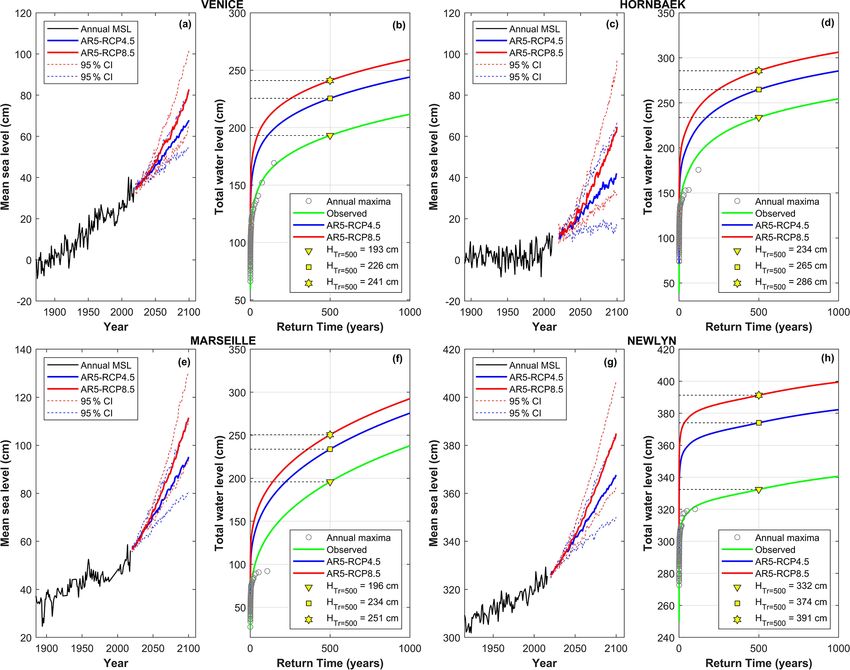
large variability in the estimates. For example, for the Venice AR5 (Church et al., 2013), which indicate an accelerating
site there is a decrease (in many cases an unbiased estimate) sea-level rise at all four observation sites (for each gauge
in the MEVD-NDE values for intermediate Tr (between 85 station under analysis, the reader can refer to the panels a,
and 105 years), while for greater Tr values (but smaller than c, e, and g in Fig. 7), with expected water level increases
Tr,max ) the error shows an overestimation of the actual quan- by the end of the century (RCP8.5) of 48 cm in Venice,
tile with respect to traditional approaches (which exhibit an 52 cm in Hornbæk, 59 cm in Newlyn, and 54 cm in Mar-
seille. The panels (b), (d), (f), and (h) in Fig. 7 show ob-
Nat. Hazards Earth Syst. Sci., 22, 1109–1128, 2022 https://doi.org/10.5194/nhess-22-1109-2022M. F. Caruso and M. Marani: Extreme-coastal-water-level estimation and projection 1121
Figure 5. Kernel density estimates for the nondimensional error (NDE) distributions obtained with a calibration sample size (S) of 30 years
and maximum return period (Tr ) at given gauge stations explored: (a) Venice (IT), (b) Hornbæk (DK), (c) Marseille (FR), (d) Newlyn (UK).
In the case of the Marseille (FR) site, MEVD parameter estimation is based (1) on non-overlapping sub-samples of fixed size (5 years; green
color) and (2) on data from the whole calibration sample (black color).
Table 3. Results of the evaluation metric obtained for all the gauge stations and for calibration sample sizes (S) equal to 5 and 30 years. In
the case of the Marseille site, text in bold refers to MEVD parameter estimation based on data from the whole calibration sample size.
S = 5 years S = 30 years
Site name Variables
BM POT MEVD BM POT MEVD
NDE median − 0.160 -0.175 − 0.178 − 0.133 − 0.158 − 0.004
Venice NDE mean − 0.069 − 0.101 − 0.116 − 0.087 − 0.133 0.024
NDE SD 0.366 0.274 0.267 0.156 0.113 0.155
NDE median − 0.119 − 0.104 − 0.113 − 0.113 − 0.115 0.056
Hornbæk NDE mean − 0.069 − 0.101 − 0.116 − 0.068 − 0.087 0.077
NDE SD 0.366 0.274 0.267 0.113 0.100 0.131
0.357
NDE median − 0.0003 0.059 0.172 0.016 0.047
0.172
0.374
Marseille NDE mean 0.045 0.129 0.262 0.013 0.050
0.183
0.178
NDE SD 0.252 0.350 0.421 0.072 0.115
0.140
NDE median − 0.010 − 0.030 − 0.033 − 0.003 − 0.032 0.0008
Newlyn NDE mean 0.003 − 0.022 − 0.026 − 0.002 − 0.031 0.002
NDE SD 0.050 0.042 0.042 0.016 0.014 0.021
https://doi.org/10.5194/nhess-22-1109-2022 Nat. Hazards Earth Syst. Sci., 22, 1109–1128, 2022You can also read