Modelling the artificial forest (Robinia pseudoacacia L.) root-soil water interactions in the Loess Plateau, China - HESS
←
→
Page content transcription
If your browser does not render page correctly, please read the page content below

Hydrol. Earth Syst. Sci., 26, 17–34, 2022
https://doi.org/10.5194/hess-26-17-2022
© Author(s) 2022. This work is distributed under
the Creative Commons Attribution 4.0 License.

Modelling the artificial forest (Robinia pseudoacacia L.)
root–soil water interactions in the Loess Plateau, China
Hongyu Li1,2 , Yi Luo1,2,3 , Lin Sun1 , Xiangdong Li4 , Changkun Ma5 , Xiaolei Wang1,2 , Ting Jiang1,2 , and
Haoyang Zhu1,2
1 Key  Laboratory of Ecosystem Network Observation and Modeling, Institute of Geographic Sciences and Natural Resources
Research, Chinese Academy of Sciences, Beijing, 100101, China
2 College of Resources and Environment, University of Chinese Academy of Sciences, Beijing, 100049, China
3 Research Centre for Ecology and Environment of Central Asia, Chinese Academy of Sciences, Urumqi, 830011, China
4 Guangdong Key Laboratory of Integrated Agro-environmental Pollution Control and Management,

Guangdong Institute of Eco-environmental Science & Technology, Guangzhou, 510650, China
5 State Key Laboratory of Eco-hydraulics in Northwest Arid Region, Xi’an University of Technology, Xi’an, 710048, China

Correspondence: Yi Luo (luoyi@igsnrr.ac.cn)

Received: 3 June 2021 – Discussion started: 23 June 2021
Revised: 7 November 2021 – Accepted: 21 November 2021 – Published: 4 January 2022

Abstract. Plant root–soil water interactions are fundamen-       the top 2.0 m layer, which was the most active zone of in-
tal to vegetation–water relationships. Soil water availabil-     filtration and root water uptake. Below this, the percentages
ity and distribution impact the temporal–spatial dynamics of     of fine roots (5.0 %) and water uptake (6.2 %) were small
roots and vice versa. In the Loess Plateau (LP) of China,        but caused a persistently negative water balance and conse-
where semi-arid and arid climates prevail and deep loess         quent DSLs. Therefore, the proposed root–water interaction
soil dominates, drying soil layers (DSLs) have been exten-       approach succeeded in revealing the intrinsic properties of
sively reported in artificial forestland. While the underlying   DSLs; their persistent extension and the lack of an opportu-
mechanisms that cause DSLs remain unclear, they hypothet-        nity for recovery from the drying state may adversely affect
ically involve root–soil water interactions. Although avail-     the implementation of artificial afforestation in this region as
able root growth models are weak with respect to simulating      well as in other regions with similar climates and soils.
the rooting depth, this study addresses the hypothesis of the
involvement of root–soil water interactions in DSLs using
a root growth model that simulates both the dynamic root-
ing depth and fine-root distribution, coupled with soil wa-      1   Introduction
ter, based on cost–benefit optimization. Evaluation of field
data from an artificial black locust (Robinia pseudoacacia L.)   Plant roots are a significant pathway in the soil–plant–
forest site in the southern LP positively proves the model’s     atmosphere continuum (SPAC), which connects the above-
performance. Further, a long-term simulation, forced by a        ground parts of the plant and the soil environment (Feddes
50-year climatic data series with varying precipitation, was     et al., 2001; Mencuccini et al., 2019) by extracting water
performed to examine the DSLs. The results demonstrate           from the soil to meet the evaporation demand of the canopy.
that incorporating the dynamic rooting depth into the cur-       This soil water uptake process is regulated by root profile
rent root growth models is necessary to reproduce soil drying    properties, which are highly dynamic in response to variable
processes. The simulations revealed that the upper bound-        soil water conditions (Schenk and Jackson, 2002; Fan et al.,
ary of the DSLs fluctuates strongly with infiltration events,    2017). In particular, forest root structures are rather com-
whereas the lower boundary extends successively with in-         plex (e.g. have woody coarse roots for anchoring and non-
creasing rooting depth. Most infiltration was intercepted by     woody fine roots for absorption) and enable diverse water ex-
                                                                 ploration strategies for adaptation to changing environments

Published by Copernicus Publications on behalf of the European Geosciences Union.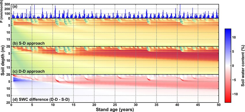
18                        H. Li et al.: Modelling the artificial forest (Robinia pseudoacacia L.) root–soil water interactions

(Mulia and Dupraz, 2006; Ivanov et al., 2012; Sivandran and         resource investment, timing and physical constraints of tree
Bras, 2013; Brunner et al., 2015). For example, in order to         rooting depth within a competitive environment”. Therefore,
increase water uptake, forests tend to grow more roots in the       they implemented variable rooting strategies and dynamic
wetter soil layers (i.e. root hydrotropism) or develop deep         root growth into the LPJmL4.0 model. Their results indicated
roots to extract deeper water resources (including deep soil        that “variable tree rooting strategies are key for modelling the
water and groundwater) (Maeght et al., 2013; Bardgett et al.,       distribution, productivity and evapotranspiration of tropical
2014; Phillips et al., 2016). The investigation also indicated      evergreen forests” in tropical South America. In their model,
that forest stands develop a complicated morphological dis-         the maximum rooting depth is estimated by the tree height
tribution of roots and diverse root water uptake strategies to      through a logistic growth function, and the vertical distribu-
adapt to the diverse soil water status conditions (Germon et        tion of the fine roots follows a shape function. Notably, the
al., 2020; Knighton et al., 2020). Therefore, plant root–soil       interactions between plant roots and soil water were not con-
water interaction is a key issue for understanding the forest–      sidered.
water relationship, which is inevitably an important part of           To meet their water requirement, plants tend to develop
ecohydrological models, fundamentally for plant water up-           more roots in water-rich zones (Germon et al., 2020). Within
take (Smithwick et al., 2014).                                      the root system, soil water is conveyed up to the above-
   Plant water uptake is usually taken as a sink term in water      ground parts through fine roots (< 2 mm in diameter) and
movement equations (Feddes et al., 2001; Clark et al., 2015).       coarse roots (> 2 mm diameter), the former for water up-
The sink term is expressed as a function of the morphologi-         take and the latter for water transport (Jackson et al., 1997;
cal and hydrological traits of the roots and soils. Morpholog-      Smithwick et al., 2014). Fine roots are developed on coarse
ically, the root profile contains two primary features, rooting     roots, together constituting a hydraulic architecture, creating
depth and vertical distribution (Warren et al., 2015), which        structural relationships for water transport (Smithwick et al.,
are commonly included in most current root uptake mod-              2014; Chen et al., 2019). According to the pipe model the-
els. These features are usually considered static in most of        ory (Lehnebach et al., 2018), for denser fine roots to take
the available hydrological and terrestrial biospheric models        up more soil water, coarser roots are required to maintain
(Luo et al., 2003; Warren et al., 2015). The maximum root-          the hydraulic transport capacity, especially for deeper exten-
ing depths are generally assumed to be static values which          sion. Balancing the cost of biomass allocation to coarse or
may differ from the plant functional types (Ostle et al., 2009).    fine roots and the benefit of the water taken up is a great
Meanwhile, the vertical root distribution is represented as an      ability of plants which live under water-stressed conditions
empirical function of root length density to soil depth over        (Guswa, 2008). Mathematical optimization methods have
the root domain (Jackson et al., 1996; Zuo et al., 2004; Sivan-     been widely implemented in previous studies to estimate the
dran and Bras, 2012), which describes the morphological fea-        optimal root profiles (Kleidon and Heimann, 1998; Collins
tures of roots statically. These simplifications of the root fea-   and Bras, 2007; Guswa, 2008; Schymanski et al., 2008, 2009;
tures allow for ease in practical applications to simulate the      Yang et al., 2016). Nonetheless, optimization efforts for root
root uptake process. However, it is increasingly recognized         dynamic processes remain limited. The coupled effects of
that efforts should be made to account for root dynamics, es-       root growth and soil water should be the fundamentals in
pecially when the coupling effects between plant growth and         the optimization approach. An optimization method will be
water availability are considered (Warren et al., 2015).            surely beneficial for simultaneously estimating the dynamics
   The dynamic roots indicate that the hydrological or terres-      of rooting depth and fine-root distribution.
trial biospheric models simulate growing roots under chang-            A drying soil layer is defined as a soil layer with a soil
ing environmental conditions, for example, soil water sta-          water content between stable field capacity and permanent
tus. This is further incorporated into the root water uptake        wilting point (Wang et al., 2011). This is a phenomenon of
models. In these process models, the dynamic root profiles          concerned and has been widely studied in the Loess Plateau
may be accounted for by either the changing rooting depth           of Northwest China. Huang and Shao (2019) reviewed the
(Gayler et al., 2014; Hashemian et al., 2015; Christina et          studies on drying soil layers in the Loess Plateau over the
al., 2017; Liu et al., 2020) or the root density distribution       past decades; this review indicated that drying soil layers pre-
(Schymanski et al., 2008; Wang et al., 2016; P. Wang et al.,        vail in the artificial forestlands in the region and develop as
2018; Drewniak, 2019; Niu et al., 2020), which is not suf-          the stand ages. It is generally believed that drying soil lay-
ficient to describe the dynamic root adaptation to changing         ers are caused by limited rainfall infiltration and improper
environmental conditions (Rudd et al., 2014). The rooting           afforestation; however, the underlying mechanisms remain
depth, root density distribution, soil water quantity, and soil     unclear and require exploration (Shao et al., 2018). Although
water spatial distribution are interrelated, and their coupling     rainfall is insufficient in the semi-arid and arid climates in the
should be reflected in the root water uptake modelling (War-        Loess Plateau, the thick loess soils store significant quantities
ren et al., 2015). Sakschewski et al. (2021) reviewed the root      of water for potential plant use. When water stress occurs in
growth approaches in the current Earth system models and            the upper soil layer due to insufficient infiltration, high at-
concluded that “none of those studies have acknowledged             mospheric demand due to the aridity may cause plants to de-

Hydrol. Earth Syst. Sci., 26, 17–34, 2022                                               https://doi.org/10.5194/hess-26-17-2022
H. Li et al.: Modelling the artificial forest (Robinia pseudoacacia L.) root–soil water interactions 19
velop roots for the use of deeper soil water (Pierret et al.,
2016). Thus, root–water interactions may play a key role in
the occurrence and development of drying soil layers.
Many in situ investigations have reported that a drying
soil layer has developed extensively in forests of black lo-
cust (Robinia pseudoacacia L.), which is the most popular
and deep-rooted afforestation species in Loess Plateau (Deng
et al., 2016; Jia et al., 2017b; Liang et al., 2018; Wu et al.,
2021). Thus, the occurrence and evolution of a drying soil
layer in this forestland are worthy of discussion. Hence, this
study aimed to (1) develop a coupled soil water–root growth
model based on the cost–benefit theory, which can simulta-
neously adjust root distribution and rooting depth in the root
water uptake model, and (2) reveal the black locust root–
soil water interactions throughout the soil profile, based on a
long-term simulation, to address the drying soil layer issues
in this region.
Figure 1. The model structure integrated from the SWAT (blue
boxes) and CLM (light orange boxes) components. The root growth
2 Materials and methods module is highlighted in yellow, and the descriptions of the dynamic
fine-root distribution and rooting depth approach are illustrated us-
2.1 Model development ing green text.
2.1.1 General description of the ecohydrological model
The root–water interaction is integrated into the root up-
Fundamentally, this ecohydrological model is an integration take model, which uses the rooting depth and fine-root distri-
of different components from the Soil and Water Assessment bution as input and acts as a sink term in the Richards’ equa-
Tool (SWAT) (Neitsch et al., 2011; Arnold et al., 2012) and tion. Soil water imposes water stress on the root growth. The
the Community Land Model version 4.5 (CLM4.5) (Oleson cost of biomass invested in coarse and fine roots and the ben-
et al., 2013) (Fig. 1). On this basis, root growth and root up- efit of water uptake were optimized through a cost–benefit
take modules were modified. Furthermore, an optimization function.
approach was introduced to simulate the coupled effects of The following sections will describe three root growth ap-
root growth and soil water dynamics. proaches in a stepwise manner: (1) the static root distribu-
Hydrologically, surface process modules, for example, tion approach implemented in CLM4.5, which assumes a
simulating evaporation, transpiration, canopy interception, static rooting depth of the coarse roots and a static distri-
and runoff, follow the SWAT model, which is detailed in its bution of fine roots (Oleson et al., 2013); (2) the approach
theoretical document (Neitsch et al., 2011). The subsurface that assumes a dynamic distribution of fine roots but a static
hydrological modules, primarily the soil water movement, rooting depth (Drewniak, 2019); and (3) the approach pro-
adopted the 1-D Richards’ equation. It is solved numerically posed in this study that assumes a dynamic distribution of
following the finite difference scheme used in CLM4.5 (Ole- fine roots and a dynamic rooting depth of coarse roots. These
son et al., 2013). three root growth modelling approaches are incorporated into
Biologically, modules for the above-ground parts, for ex- the ecohydrological model mentioned above for a compari-
ample, plant phenology, leaf area index (LAI) development, son of their performances.
and biomass accumulation, are adopted from SWAT (Neitsch
et al., 2011) and CLM4.5 (Oleson et al., 2013). The mod- 2.1.2 Static distributions of coarse and fine roots
ule for the below-ground part, the root growth model, simu-
lates root growth following CLM4.5 which, in turn, adopts In this approach, a static exponential function expresses the
the approaches from process simulation directly from the root fractions in different soil layers (Zeng, 2001):
implementation in the Biome-BGC (Biome BioGeochemical
Cycles) model (Thornton et al., 2002). See the Supplement 0.5 exp −ra zh,i−1
+ exp −rb
zh,i−1
for more information on the detailed model descriptions. In fri = − exp
−ra zh,i − exp −rb zh,i 1≤i
20                              H. Li et al.: Modelling the artificial forest (Robinia pseudoacacia L.) root–soil water interactions

of soil layer i, and ra and rb are two shape parameters. The            (1) Carbon allocation between the coarse and fine roots
shape parameters can be obtained by fitting to the observa-
tions for different plant types and are set as 4.8 and 0.8 ac-          The cost is defined as the amount of carbon invested to grow
cording to fine-root sampling in this study (see Sect. 2.2.4)           coarse/fine roots. In constructing the coarse-root and fine-
respectively (Oleson et al., 2013).                                     root systems, the pipe model theory (PMT; Shinozaki et al.,
                                                                        1964) was adopted. Lehnebach et al. (2018) summarized “the
2.1.3    Dynamic distribution of fine roots                             essence of the PMT concept” as “a unit amount of leaves
                                                                        is provided with a pipe whose thickness or cross-sectional
This approach assumes that newly assimilated biomass to the             area is constant. The pipe serves both as the vascular pas-
below-ground parts is allocated to develop fine and coarse              sage and as the mechanical support and runs from the leaves
roots with a static ratio. In general, there is a linear relation-      to the stem through all intervening strata.” The relationship
ship between the carbon mass and biomass (Niu et al., 2020).            between the leaf and stem can be established quantitatively
Therefore, the term “carbon” will be used in the following              based on the PMT and can be extended to the below-ground
text to refer to the biomass of different plant components.             parts of the plants (Chen et al., 2019). For roots, the rela-
Within the present rooting depth (which is static over the              tionships have been established in analogue form and vali-
simulation period), the fine roots are distributed over the soil        dated against some databases (Carlson and Harrington, 1987;
depth according to the soil water content. In each soil layer i,        Richardson and Dohna, 2003).
the fine-root carbon increment is updated at each time step,               Delineating the soil profile into adjacent soil layers which
as follows:                                                             correspond to the numerical solution of the Richards’ equa-
FRi,t = FRi,t−1 + 1FRi,t ,                                      (2)     tion, the equations for modelling the root growth are also
                                                                        written regarding the discrete soil layers (Fig. 2c).
where FRi,t−1 (g m−2 d−1 ) is the fine-root carbon of soil                 The carbon amount for coarse and fine roots should be
layer i during the previous time step, and 1FRi,t (g m−2 d−1 )          maintained as
is the newly allocated carbon to fine roots of soil layer i at
time t. 1FRi,t is modified by the soil water content as fol-            CR0i = ρ · Zi · kA · FRi ,                                  (6)
lows:
                     THKi REWi                                          where CR0i is the equivalent carbon for coarse roots in the
1FRi,t = 1FR · n                     ,                     (3)          zone between the ground surface and bottom of soil layer i,
                   P
                      (THKi REWi )                                      FRi is the carbon for fine roots within soil layer i, ρ is the
                          i=1
                                                                        mass density of coarse roots (g cm−3 ), Zi is the depth from
where 1FR is the newly assimilated carbon allocated to total            the surface to the bottom of soil layer i (cm), and kA is a con-
fine roots (g m−2 d−1 ), n is the total number of soil layers           stant which can be determined from field observations (see
in the rooting zone, THKi is the soil layer thickness of soil           Sect. 2.3.2).
layer i (cm), and REWi is the relatively effective soil water              For an increment of carbon for fine roots within soil
content (i.e. soil water availability). REWi is calculated as           layer i, a corresponding increment of carbon for coarse roots
follows:                                                                is needed and can be derived from Eq. (6):
           θ − θwp
REWi =              ,                                     (4)           1CR0i = ρ · Zi · kA · 1FRi .                                (7)
          θfc − θwp

where θ is the soil water content (cm3 cm−3 ), and the sub-             Notably, there is no increment of carbon for coarse roots if
scripts “wp” and “fc” indicate the soil water content at the            the available coarse roots are sufficient to support the new
wilting point and field capacity respectively.                          fine roots, as discussed later.
   The fine-root fraction in each soil layer i is then calculated:         The increments of carbon for fine and coarse roots were
                                                                        then summed over the root profile:
         FRi,t
fri =   n             .                                         (5)
        P                                                                        n
              FRi,t                                                              X
        i=1                                                             1CR =         1CR0i ,                                       (8)
                                                                                1
2.1.4    Dynamic distributions of coarse and fine roots                         n
                                                                                X
                                                                        1FR =         1FRi .                                        (9)
This approach assumes that both the rooting depth of coarse                       1
roots and the distribution of fine roots change with soil water.
In formulating the growth of the coarse and fine roots, the             The sum of the newly allocated carbon for fine and coarse
newly allocated biomass/carbon for the below-ground part                roots is equal to that allocated to the below-ground part 1TR:
is optimally allocated to the roots based on a cost–benefit
function that will be described in detail.                              1FR + 1CR = 1TR.                                           (10)

Hydrol. Earth Syst. Sci., 26, 17–34, 2022                                                      https://doi.org/10.5194/hess-26-17-2022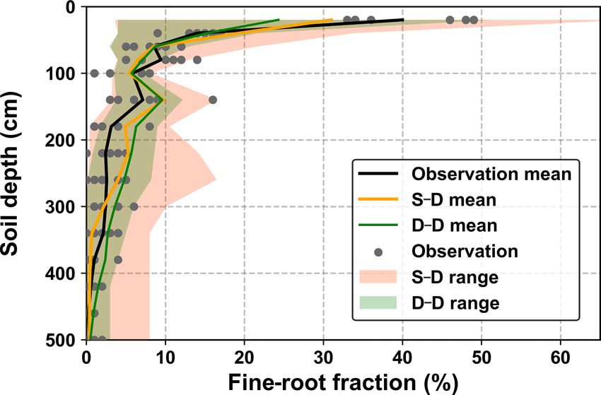
H. Li et al.: Modelling the artificial forest (Robinia pseudoacacia L.) root–soil water interactions                                           21

Figure 2. (a) Black locust root system obtained from an experimental pot; (b) scanned image of one root segment consisting of coarse and
fine roots; (c) schematic description of pipe model theory adopted for coarse and fine roots; (d) weighting factors for carbon allocation and
conceptualized benefit (available soil water for uptake) and cost (carbon investment).

Two respective ratios are defined for fine and coarse roots as           Updating the fine-root fractions using Eq. (7), the demand for
follows:                                                                 coarse roots that can meet the hydraulic transport demand for
                                                                         the fine roots within and below soil layer i is
          1FR               1CR
KFR =             , KCR =           .                          (11)                n                        n
        1CR + 1FR         1CR + 1FR                                                X                        X
                                                                         CRPi =               CR0i ,NEW =          ρ ·Zi ·kA ·(FRi + 1FRi ) . (16)
(2) Spatial distribution of new fine and coarse roots                                  j =i                 j =i

Potentially, more fine roots develop in wetter soil zones in             Comparing the demand for and current storage of coarse
order to gain more water and to reduce water stress as much              roots, the coefficient of the coarse-root carbon increment re-
as possible. It is fundamentally recognized that penetration             garding the soil layer i is calculated as
into deeper soil requires carbon for the fine roots, as well as                   max (CRPi − CRi , 0)
the corresponding coarse roots; the potential benefit can be             βi =    n                      .                                    (17)
                                                                                 P
more water uptake from the deeper soil. The basic principle                        max (CRPi − CRi , 0)
                                                                                 i=0
for the distribution of the roots, either fine only or both coarse
and fine, is that an optimal distribution of new roots helps to          According to Eq. (11), the increment of carbon for the coarse
gain as much water as possible (Fig. 2d).                                roots with respect to each soil layer is then calculated as
   Thus, the distribution of fine roots is influenced by a cost–
benefit ratio, which is defined as follows:                              1CRi = 1TR · KCR · βCi .                                            (18)

       REWi                                                              (3) Rooting depth extension
Wi =        ,                                                  (12)
       CFRi                                                              To calculate the rooting depth extension via optimization, the
where Wi is the cost–benefit ratio in soil layer i, and the ben-         target function Sm is defined as follows:
efit is presented by REWi , as defined previously. CFRi is                       m
                                                                                 X
defined as the marginal carbon cost of fine roots:                       Sm =           (THKi · fri · REWi ) .                               (19)
                                                                                i=1
          ∂ 1CR0i + 1FRi
CFRi =                        = ρ · Zi · kA + 1.            (13)         When Sm reaches its maximum, the optimum distribution of
                ∂1FRi                                                    new roots over the soil profile is obtained. If Sm reaches its
Combining Eqs. (13) and (12),                                            maximum when m is equal to n, the length of the coarse root
                                                                         remains unchanged; however, when m is equal to n + 1, the
           REWi                                                          coarse root penetrates the next soil layer.
Wi =                   .                                       (14)
       ρ · Zi · kA + 1
                                                                         2.2     Data
Replacing REWi with Wi in Eq. (3), the fraction of new fine
roots in the soil layer i becomes                                        2.2.1    Site description

                    THKi Wi                                              The study site is located in the Yeheshan Provincial Na-
1FRi = 1FR ·                    .                              (15)
                  m
                  P                                                      ture Forest Reserve (34◦ 31.760 N, 107◦ 54.670 E; 1090 m el-
                     (THKi Wi )
                 i=1                                                     evation) in the southern part of the Loess Plateau in China

https://doi.org/10.5194/hess-26-17-2022                                                           Hydrol. Earth Syst. Sci., 26, 17–34, 2022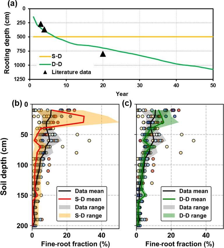
22                         H. Li et al.: Modelling the artificial forest (Robinia pseudoacacia L.) root–soil water interactions

Figure 3. (a) Location of the study site (Yeheshan) in the Loess Plateau, China; (b) top view from the black locust plantation canopy in
July 2018; (c) meteorological observation tower, soil moisture observation, and excavation root profile; (d) installation of the soil moisture
sensors.

(Fig. 3). The climate is semi-humid with an annual average
temperature of 11.3 ◦ C and precipitation of 570 mm (from
Yongshou station; see Sect. 2.2.2). It is hot in summer and
cold in winter, and precipitation occurs predominantly from
May to October with significant inter-annual variation. Ar-
tificially afforested black locust (Robinia pseudoacacia L.)
dominates the vegetation species with an average height of
10 m (planted in 2000) and a density of 2450 trees ha−2 (Ma
et al., 2017). The experimental plots were situated within
a black locust forestland on an average slope of 8◦ . Instru-
ments for the microclimate and soil water observations were              Figure 4. Time series of annual precipitation (mm). The dashed
installed. The thickness of the loess soil is estimated to be            coloured lines represent the average values (AVE) and ±1 standard
more than 50 m, and the buried depth of groundwater is be-               deviation (SD).
yond that depth (Liu et al., 2010).

2.2.2   Meteorology                                                         In addition, daily meteorological data for 1971 to 2020
                                                                         from the National Metrological Station in Yongshou County,
A meteorological observation system was established on a                 26 km from the field experiment site, were downloaded from
flux tower in 2014. The tower was 16 m above the ground,                 the China Meteorological Data Service Centre (http://data.
higher than the tree canopy (Fig. 3). This system consists               cma.cn, last access: 23 March 2021) for the long-term sim-
of HMP155A probes (Campbell Scientific, Inc., Logan, UT,                 ulation. The data series include daily precipitation, mean air
USA) for temperature and humidity, a CSAT3 3-D ultra-                    temperature, maximum air temperature, minimum air tem-
sonic anemometer (Campbell Scientific, Inc., Logan, UT,                  perature, relative humidity, wind speed, and sunshine hours.
USA) for wind speed, and a CNR4 net radiometer (Camp-                       It is believed that the data series, spanning 50 years, covers
bell Scientific, Inc., Logan, UT, USA) for solar radiation. A            the inter-annual variations in climatic factors, especially the
T-200B precipitation gauge (Geonor Inc., Oslo, Norway) was               alternating wet and dry periods (Fig. 4). The annual average
installed near the forest opening to measure throughfall. A              precipitation is 570 mm, with a standard deviation (SD) of
CR3000 data logger (Campbell Scientific, Inc., Logan, UT,                122 mm.
USA) was used to collect data from the sensors at 10 min
intervals.

Hydrol. Earth Syst. Sci., 26, 17–34, 2022                                                      https://doi.org/10.5194/hess-26-17-2022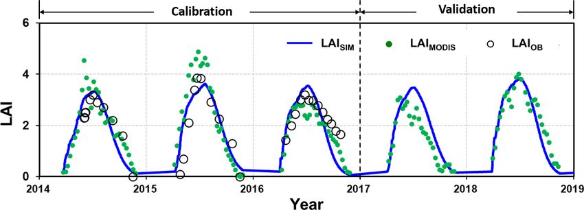
H. Li et al.: Modelling the artificial forest (Robinia pseudoacacia L.) root–soil water interactions                               23

2.2.3   Soil and water                                                  The measured LAI values were compared to those of the
                                                                     Moderate Resolution Imaging Spectroradiometer (MODIS)
The soil properties were investigated by sampling over a pro-        MYD15A2H product, which has a spatial resolution of
file 5.0 m below the ground at the study site. The dry bulk          500 m and a temporal resolution of 8 d. Furthermore, the 8 d
density (ρb , g cm−3 ) was obtained by drying volumetric soil        MODIS LAI series were downscaled to a daily series using
samples (100 cm3 ) at 105 ◦ C for 48 h, and the soil particle        the Savitzky–Golay filtering technique (Tie et al., 2017).
size distribution and organic matter content were measured              The root profiles were investigated in August 2015. A
in the laboratory. Silt loam dominated the profile, with mod-        150 cm wide trench, which was located between two neigh-
erate variations among the soil layers. On average, the silt         bouring rows and perpendicular to the row direction, was ex-
loam consisted of 5.8 % sand, 73.4 % silt, and 20.9 % clay           cavated 500 cm below the ground (Fig. 3). During the exca-
(Ma et al., 2017).                                                   vation, soil samples, 20 cm in the horizontal dimension and
   The saturated hydraulic conductivity (Ks , cm h−1 ) was           40 cm in vertical thickness, were taken along the trench and
measured in the undisturbed soil samples using a constant-           over the profile. It is assumed that the roots develop homo-
head method (Ramos et al., 2017). The field capacity (θfc )          geneously along the horizontal row but unevenly along the
and wilting point (θwp ) were derived from the power function        trench. Finally, seven samples were collected from each soil
(Campbell, 1974; Clapp and Hornberger, 1978), correspond-            layer across the trench. The soil samples were rinsed, and the
ing to the soil potentials of −33 and −1500 kPa respectively.        weight and length of fine roots (less than 2 mm in diameter)
   Volumetric soil moisture sensors were installed in 14 lay-        were measured for each sample.
ers within a depth of 500 cm from the surface: at 5, 15, 30,            To estimate the parameters of the black locust root system,
45, 60, 90, 120, 150, 200, 250, 300, 350, 400, and 500 cm            a pot experiment was carried out in 2016 (planted in April
respectively (Fig. 3). The sensors, CS-655 soil water content        and sampled in October), the details of which are given in
reflectometers (Campbell Scientific, Inc., Logan, UT, USA),          Fig. S1 in the Supplement.
have been in operation since June 2014. A CR1000 data log-              In addition to the measurements mentioned above, data on
ger (Campbell Scientific, Inc., Logan, UT, USA) records the          black locust roots, including the density profile and rooting
data every 10 min.                                                   depth were compiled from the published literature (see Sup-
   The soil properties below 5.0 m were adopted from previ-          plement).
ous studies (Li et al., 2008; Jia et al., 2017a; Wu et al., 2021)
on black locust plantations in the Loess Plateau.                    2.3     Model set-up
   The soil desiccation index (SDI) was used to evaluate the
degree of soil desiccation for the comparison between the            2.3.1    Initial and boundary conditions for the Richards’
observation and simulation results; this index was calculated                 equation
as follows:
         θ − θwp                                                     In solving the Richards’ equation numerically, the vertical
SDI =              ,                                         (20)    domain extends from the surface to 20 m below the ground.
        θsfc − θwp
                                                                     The domain was discretized into adjoining layers with a
where θsfc is the soil water content at a stable field capacity.     thickness of 5 cm each.
In practice, a soil water content at 60 % of field capacity (θfc )      The upper boundary condition was set as the flux of the
can be assumed to be the stable field capacity of loess in           rainfall rate with the canopy interception removed or the soil
the Loess Plateau (Wang et al., 2011). Soil layers with an           evaporation rate. As the soil water content in deep soil (20–
SDI < 1 were regarded as drying soil layers.                         100 m) is relatively stable around the field capacity (Qiao et
                                                                     al., 2018), the lower boundary was set to a constant soil water
2.2.4   Plants                                                       content at the field capacity.
                                                                        During the calibration and validation stages, the initial soil
The leaf area index (LAI, m2 m−2 ) of the black locust canopy        water profile was determined using the measurements. The
was measured using an optical method (Jonckheere et al.,             initial soil water profile was set at the field capacity when the
2004), biweekly or triweekly during the growing seasons              model was applied to the long-term simulation.
of 2014, 2015, and 2016. An 8 mm fisheye lens (Sigma
F3.5 EX DG circular fisheye, Sigma Corporation) mounted              2.3.2    Numerical simulations
on a Canon EOS 5D digital SLR camera (http://www.canon.
com, last access: 20 December 2020) took hemispherical               The soil hydraulic parameters, saturated hydraulic conductiv-
photographs of the canopy on cloudy days. The photographs            ity Ks and constant B in the soil water retention curve, were
were analysed using the CAN_EYE software to derive the               initialized by the measured values. They were further tuned
LAI values (Demarez et al., 2008). Within each plot, pho-            to match the simulated soil water content to the observations.
tographs were taken at five different positions each time. The          The vegetation growth parameters were adapted from
LAI value for the plot is the average of the five positions.         Zhang et al. (2015), who simulated the black locust growth

https://doi.org/10.5194/hess-26-17-2022                                                 Hydrol. Earth Syst. Sci., 26, 17–34, 2022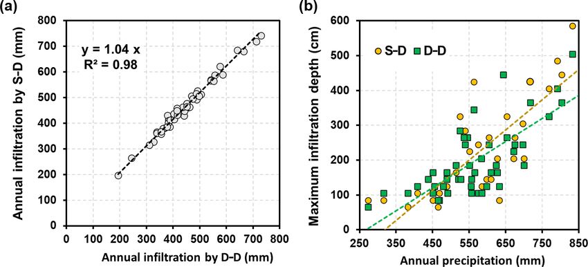
24                              H. Li et al.: Modelling the artificial forest (Robinia pseudoacacia L.) root–soil water interactions

in the Loess Plateau using the Biome-BGC model. Other                               n
                                                                                    P
vegetation parameters were obtained from the SWAT model                                   (Si − Oi )
                                                                                    i=1
(Neitsch et al., 2011; Sun et al., 2011).                               PBIAS =           n            × 100 %.                     (23)
                                                                                          P
   All the relevant parameters are summarized in Table S1 in                                    Oi
the Supplement.                                                                           i=1

2.3.3   Numerical simulations                                           Here, Si is the simulated value at time step i, S is the mean of
                                                                        the simulated value, Oi is the observed value at time step i,
The numerical simulations consist of two parts, the short-              O is the mean of the observed value, and n is the number of
term (5 years) simulation for model calibration and valida-             time steps. R 2 and NSE were dimensionless. The dimension
tion, and the long-term simulation (50 years) for investiga-            of the PBIAS was percent (%).
tion:                                                                      R 2 describes the proportion of the variance in the mea-
                                                                        sured data explained by the model, ranging from 0 to 1,
 1. The model calibration and validation were performed                 with higher values indicating less error variance. The NSE
    for the observation period (2014–2018). The model was               indicates the consistency between the plot of the ob-
    calibrated from 1 June 2014 to 31 December 2016 and                 served vs. simulated data and the 1 : 1 line, ranging be-
    validated through 1 January 2017 to 31 December 2018.               tween −∞ and 1.0 (1 inclusive) and optimized at the
    The measured LAI, soil water content, and root pro-                 value of 1. The PBIAS measures the average tendency
    files were used for the evaluation. The rooting depth               of the simulated data to be larger or smaller than the
    was assumed to be 5.0 m below the ground for three ap-              observation, and a lower value implies a more accurate
    proaches, considering the relatively short period of the            model simulation, with optimization at 0.0. Positive val-
    field experiment.                                                   ues indicate a model underestimation bias, and negative
 2. A long-term simulation was performed to explore the                 values indicate a model overestimation bias. Moriasi et
    forest root–soil water interactions over a period of                al. (2007) proposed a widely used rating system, which
    50 years, with the aim of investigating the drying soil             judged the modelling performance as “very good”, “good”,
    layer evolution over the long term considering inter-               “satisfactory”, or “unsatisfactory” using PBIAS < ±10 %,
    annual variation in precipitation. The long-term simula-            ±10 % ≤ PBIAS < ±15 %, ±15 % ≤ PBIAS < ±25 %, or
    tion adopted the data from Yongshou Station for 1971–               PBIAS ≥ ±25 % respectively or using 0.75 < NSE ≤ 1.0,
    2020 without any sense of a specific historical period.             0.65 < NSE ≤ 0.75, 0, 0.50 < NSE ≤ 0.65, or NSE ≤ 0.50 re-
    In the long-term simulation, a value of 5.0 m was set               spectively.
    for the rooting depth of the static approaches; an initial
    value of 50 cm was set for the dynamic rooting depth                3     Results
    approach. Plants start to grow at the beginning of the
    simulation.                                                         3.1    Model calibration and validation

2.3.4   Evaluation indices                                              The model parameters, maximum LAI (LAImax ), saturated
                                                                        hydraulic conductivities (Ks ), and exponent of the soil–water
Statistical indices, the coefficient of determination (R 2 ),           characteristic curve (B), were calibrated and validated us-
the Nash–Sutcliffe efficiency (NSE), and the percent                    ing the field measurements. The initial value of the LAImax
bias (PBIAS), were used to evaluate model performance and               was assigned a default of 5.0 in the SWAT model; the ini-
are given as follows:                                                   tial values for Ks and B were based on measurements in the
         n
         P                                                            laboratory of the samples taken from the field site. The soil
                Si − S Oi − O                                           hydraulic parameters varied for the different soil layers. The
         i=1                                                            calibration was performed manually using the observed LAI
R2 = s                                       ;                 (21)
         n
         P               n
                        P                                             and soil water content as the target. The performance was
               Si − S           Oi − O                                  evaluated using the indices mentioned in the previous sec-
         i=1              i=1
               n
                                                                        tion, and the calibrated values are listed in Table S1.
               P
                     (Oi − Si )2                                           The simulated LAI values were plotted against the field
               i=1                                                      measurements for 2014–2016 for calibration and 2017–
NSE = 1 −       n                    ;                         (22)
               P                2                                      2018 for validation (Fig. 5). Further, the MODIS-derived
                     Oi − O
               i=1
                                                                        LAI values were used for evaluating the simulation over the
                                                                        entire period as well, especially for the validation period
                                                                        of 2017–2018, for which the field measurements were not
                                                                        available.

Hydrol. Earth Syst. Sci., 26, 17–34, 2022                                                        https://doi.org/10.5194/hess-26-17-2022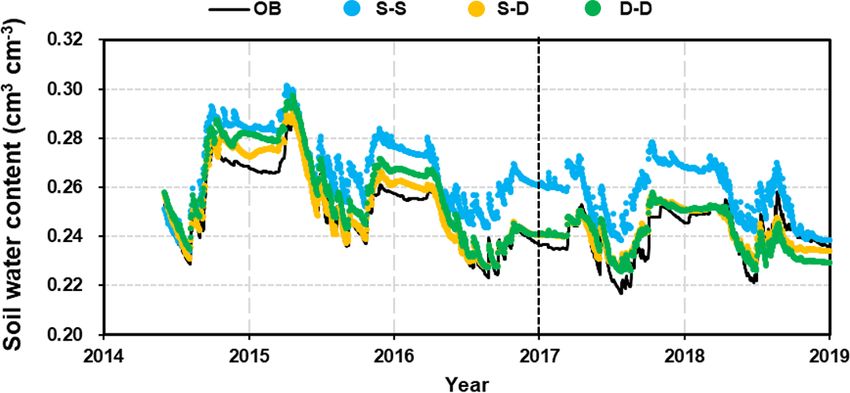
H. Li et al.: Modelling the artificial forest (Robinia pseudoacacia L.) root–soil water interactions                              25

Figure 5. Comparison of the leaf area index (LAI) from simu-
lation (LAISIM ), MODIS-derived data (LAIMODIS ), and plot ob-
servation (LAIOB ) for the calibration (2014–2016) and valida-    Figure 6. Comparison of the 5 m profile-averaged soil water con-
tion (2017–2018) periods.                                         tent (SWC) from observations (OB) and the three root simula-
                                                                  tion approaches during the calibration (2014–2016) and valida-
                                                                  tion (2017–2018) periods. The abbreviations used in the figure are
   During the calibration period, the simulated LAI values fit    as follows: S–S – static rooting depth and static fine-root distri-
the measurements with a classification of “very good” (Mo-        bution; S–D – static rooting depth and dynamic fine-root distribu-
riasi et al., 2007), with an NSE of 0.60 and a PBIAS of           tion; D–D – dynamic rooting depth and dynamic distribution of fine
5.2 %. Validation with the MODIS-derived LAI indicated a          roots.
“very good” performance (Moriasi et al., 2007), with an NSE
of 0.80 and a PBIAS of 17.5 %.
   The MODIS-derived LAI exhibited remarkably similar                The evaluation indices R 2 values for the static and dy-
seasonal patterns to the field measurements. Over- or un-         namic rooting depth approaches were 0.96 and 0.96, the NSE
derestimation was also noticed, for example, in 2014–2016         values were 0.91 and 0.71, and PBIAS values were 1.2 %
and 2017 respectively (Fig. 5). Other studies have reported       and 2.9 % respectively at the calibration stage; at the valida-
that overestimation may specifically occur for the LAI dur-       tion stage, the R 2 values were 0.66 and 0.64, the NSE values
ing the wet season when compared with the field experiments       were 0.66 and 0.58, and the PBIAS values were 7.0 % and
(Yang et al., 2006; Naithani et al., 2013) or when cross-         0.4 % respectively. This model performance can be catego-
evaluated against other remote-sensing-based products (Gar-       rized as “good” or “very good” following the rating system
rigues et al., 2008). The simulation demonstrated an overesti-    by Moriasi et al. (2007).
mation of the LAI when compared with the MODIS-derived               The fine-root density profiles produced during the calibra-
LAI in 2017. Although it is also argued that the MODIS-           tion and validation stages were compared with the sampled
derived LAI may underestimate reality (Fang et al., 2012), it     values obtained in August 2015 (Fig. 7). The measured fine-
is not sure which one (or both) is responsible for the discrep-   root densities varied significantly among the seven sampled
ancy between the simulated and observed values in 2017 due        profiles, and the variations decreased with soil depth. The
to the unavailability of field measurements. The point-pixel      simulated fine-root densities exhibited an even wider range
comparison issue might also be a reason for the quantitative      of variations, which covered the growth seasons from 2014
difference between the MODIS-derived and field-measured           to 2018. On average, the root distribution of the dynamic
LAI. Nevertheless, the evaluation indices indicate the accep-     rooting depth approach was closer to the measurements than
tance of the LAImax by the model performance in both the          that of the static rooting depth approach.
calibration and validation stages.                                   Variations in fine-root distribution simulated by the static
   Figure 6 shows a simplified comparison of the average          and dynamic rooting depth resulted from strategies for sim-
soil water content (SWC) over the 5.0 m profile, which illus-     ulating the root–soil water interactions. In the static rooting
trates the differences among the root growth simulations. The     depth approach, the growth of fine roots was purely deter-
simulations reproduced the patterns in the SWC throughout         mined by soil water availability and its distribution within the
the seasons and between rainfall events exceptionally well        rooting domain, for example, 5.0 m in this study (see Eqs. 3
in both the calibration and validation stages. The dynamic        and 5 in Sect. 2.1.4). In contrast, in the dynamic rooting depth
fine-root distribution approaches (S–D and D–D, which re-         approach, growth of the fine roots may demand an increment
fer to the static rooting depth and dynamic fine-root distri-     of coarse roots that will cost more carbon and is finally de-
bution approach and the dynamic rooting depth and dynamic         termined by the optimization of the cost–benefit functions,
distribution of fine-roots approach respectively) reproduced      as described by Eqs. (12) and (18). Thus, the dynamic root
the variations in SWC remarkably well; however, the static        depth approach resulted in a narrower variation range than
rooting depth and static fine-root distribution (S–S) approach    the static rooting depth approach. Averaged over the simu-
deviated significantly. Therefore, the results of this approach   lation period, the dynamic rooting depth approach achieved
will no longer be discussed in the following sections.            a more homogeneous fine-root distribution profile than the
                                                                  static rooting depth approach, implying that the former ap-

https://doi.org/10.5194/hess-26-17-2022                                              Hydrol. Earth Syst. Sci., 26, 17–34, 2022
26 H. Li et al.: Modelling the artificial forest (Robinia pseudoacacia L.) root–soil water interactions
Figure 7. Comparison of the 5 m profile-averaged soil water con-
tent (SWC) from observations (OB) and the two root simulation ap-
proaches during the calibration (2014–2016) and validation (2017–
2018) periods. The abbreviations used in the figure are as follows:
S–D – static rooting depth and dynamic fine-root distribution; D–D
– dynamic rooting depth and dynamic distribution of fine roots.
proach utilized more soil water from the deeper soil layers. Figure 8. Evaluation of the simulated root distribution against the
This point will be further addressed in the discussion regard- literature data: (a) rooting depth, (b) fine-root distribution in the top
ing the drying soil layer evolution over the long term. 2.0 m soil layer for the static rooting depth approach (S–D), and
(c) fine-root distribution in the top 2.0 m soil layer for the dynamic
3.2 Long-term simulation rooting depth approach (D–D). The scatters with different colours
illustrate the observational data from different literature sources,
3.2.1 Rooting depth and soil water and the shaded areas illustrate the range of the mean ± standard de-
viation of simulation.
Simulations forced by the long-term climatic data series re-
vealed root development using the static and dynamic root- nificant difference in root–water interactions. The soil water
ing depth approaches (Fig. 8a). Instead of assigning a fixed varied significantly with precipitation during the entire pe-
root depth of 5.0 m in the static rooting depth approach, the riod. In most years, the maximum infiltration depth was less
dynamic rooting depth approach simulated the root depth ex- than 2.0 m. Meanwhile, precipitation could infiltrate down to
tension, which is consistent with the data from the literature. 5.0 m in consecutive wet years, for example, the period from
It was found that the rooting depth may be as deep as 11.0 m the 10th to 15th years. Notably, a time lag effect existed be-
below the ground. The simulated rooting depth extension rate tween the peak precipitation and the maximum infiltration
slowed as the stand age increased, which was also consis- depth: the peak precipitation occurred around August, while
tent with the observations in artificial forests (see in Fig. S4; the maximum infiltration depth was reached around March
Christina et al., 2011; Wang et al., 2015). Furthermore, the in the following year.
simulated root profiles by the two approaches within a 2.0 m
soil depth were also evaluated against the data collected from 3.2.2 Infiltration
the literature (Fig. 8b, c). The simulated results varied within
the range provided by the data in the literature. Regressions Precipitation replenishes soil water through infiltration. The
between the mean fine-root fractions by the static and dy- amount and depth of the infiltrated water impact the growth
namic rooting depth approaches and that of the literature data and water use of the root systems. The infiltration is associ-
provided R 2 values of 0.34 and 0.64 respectively, indicating ated with the a priori soil water content and its distribution
that the dynamic approach performed better than the static over the profile, the amount and duration of an individual
approach. precipitation event, and the effects of the randomly sequen-
The evolution of root growth and soil water over the long tial events. Establishing a relationship between the infiltra-
term is depicted in Fig. 9. Visually, wetting and drying pro- tion depth and precipitation on the basis of a single event is
cesses over the soil profiles were commonly found from sim- complicated and difficult to achieve. Instead, analyses were
ulations of both root growth modelling approaches. However, performed on an annual basis; that is, the maximum infiltra-
the difference in the simulated soil water distribution was tion depth vs. the annual precipitation amount were regressed
also significant (Fig. 9d). for the two root growth modelling approaches, as shown in
These two approaches resulted in substantially different Fig. 10. During the simulation period of 50 years, the annual
spatial distributions of roots and soil water and, thus, a sig- precipitation varied from 250 to 850 mm. It was found that
Hydrol. Earth Syst. Sci., 26, 17–34, 2022 https://doi.org/10.5194/hess-26-17-2022H. Li et al.: Modelling the artificial forest (Robinia pseudoacacia L.) root–soil water interactions 27
Figure 9. Time series of (a) monthly precipitation (mm per month), (b) soil water content (SWC) along the 20 m soil profile simulated by
the static rooting depth (S–D) approach, (c) soil water content along the 20 m soil profile simulated by the dynamic rooting depth (D–D)
approach, and (d) the difference in the SWC between the S–D and D–D approaches. The dashed black horizontal line in panel (b) and the
curve in panel (c) indicate the rooting depth.
Figure 10. Comparisons of (a) infiltration amounts and (b) maxi- Figure 11. Profile of (a) fine-root density distributions (%) and
mum infiltration depths between the static rooting depth (S–D) and (b) root water uptake distributions (mm) resulting from different ap-
dynamic rooting depth (D–D) approaches. proaches (the S–D and D–D approaches). The error bars represent
the standard error (SE) of the mean of different years.
the annual infiltration amounts from these two approaches
were exceptionally close to each other. The dynamic rooting
depth approach was 4.0 % lower than that of the static rooting 3.2.3 Fine-root distribution and water uptake
depth approach, which is an insignificant difference, as dis-
cussed in a later section. The maximum infiltration depth was The fine-root distributions simulated by these two ap-
positively correlated with the annual precipitation, which is proaches showed exceptionally similar patterns in the soil
not uncommon. The results also indicated that the maximum profile (Fig. 11a). However, a quantitative difference between
infiltration depth may reach 6.0 m below the ground in very them was also noticeable. For the static rooting depth ap-
wet years. Interestingly, the regression lines of these two proach, roots grow only within the soil layer with a present
root growth modelling approaches crossed at approximately 5.0 m thickness. For the dynamic rooting depth approach, the
500 mm of annual precipitation. When annual precipitation coarse roots reach 11.0 m below the ground. Within the top
was less than 500 mm, the infiltration reached deeper soil for 2.0 m soil layer, the fractions of fine roots for the static and
the static rooting depth approach, and the inverse was found dynamic rooting depth approaches were 90.0 % and 80.3 %
when the annual precipitation was more than 500 mm. respectively, and within the 2.0–5.0 m soil layer, these values
were 10.0 % and 14.7 % respectively. For the dynamic root-
ing depth approach, only 5.0 % of fine roots were in the soil
below 5.0 m.
The distribution of root water uptake over the soil profile
was similar to that of the fine-root density (Fig. 11b). The
https://doi.org/10.5194/hess-26-17-2022 Hydrol. Earth Syst. Sci., 26, 17–34, 202228 H. Li et al.: Modelling the artificial forest (Robinia pseudoacacia L.) root–soil water interactions static rooting depth approach resulted in an annual water up- study site in the Loess Plateau, it was reported that the thick- take of 338 mm (SD = 84 mm), whereas the dynamic rooting ness of the drying soil layer reached 7.0 m, with its lower depth approached 381 mm (SD = 84 mm). In the top 2.0 m boundary as deep as 8.0 m below the ground in the black lo- soil layer, the root uptake was 298 and 318 mm for the static cust plantation (Li et al., 2008). It should also be noted that and dynamic rooting depth approaches respectively. In the the sampling depth was limited to 8.0 m. Deep sampling has 2.0–5.0 m layer, the values for the static and dynamic root- indicated that drying soil layers reach a depth of 19.0 m in ing depth approaches were 40 and 40 mm respectively. Be- the Loess Plateau (Wu et al., 2021). low 5.0 m, the dynamic approach resulted in a root uptake of 24 mm, which accounted for 6.2 % of the uptake from the entire profile. 4 Discussion 3.2.4 Evolution of drying soil layers 4.1 Root–water interactions and drying soil layers The long-term soil water evolution is illustrated in Fig. 9. As indicated in Sect. 1, this study attempted to develop a Vertically, the most active soil water zone was within the root growth model that can simulate coarse-root extension top 2.0 m (statistically based on the simulation results). This dynamically instead of the static rooting depth approach cur- was confirmed by root development and water uptake in this rently adopted in most available models (Sivandran and Bras, study (Fig. 11) and by field observations in this region (Suo 2013; Wang et al., 2016; P. Wang et al., 2018; Drewniak, et al., 2020). In the top 2.0 m soil layer, infiltration events re- 2019; Niu et al., 2020). In formulating the dynamic rooting plenish and plant roots deplete the soil water alternately. The depth, the study proposed a cost–benefit algorithm based on two root growth modelling approaches resulted in remark- ecophysiological principles (Chen et al., 2019). The evalu- ably similar soil water enrichment and depletion patterns in ation of the simulated results against the field observations the top 2.0 m layer, especially during the infiltration period from this study and from the literature proved its effective- (Fig. 9d). Below the top 2.0 m, soil water was continuously ness for the Loess Plateau. in a negative state, and the dynamic rooting depth approach The static rooting depth approach is widely used in eco- resulted in more soil water depletion than the static rooting logical and hydrological models, which have been employed depth approach. to simulate soil water variations in field crops, shrubs, and Drying soil layers have been frequently reported in previ- forests in the Loess Plateau (Zhang et al., 2015; Tian et al., ous studies in the Loess Plateau (Y. Wang et al., 2018). The 2017; B. Li et al., 2019; Bai et al., 2020). Short-term model upper and lower boundaries of the drying soil layers were calibration and validation, ranging from months to 5 years, defined according to the soil desiccation index (Wang et al., have usually shown acceptable performance, whereas long- 2011), as shown in Fig. 12. The static rooting depth approach term evaluation has rarely been undertaken. When used to did not demonstrate the sustainable existence of drying soil address the long-term issue in this study, comparisons be- layers. This is because it pre-sets a fixed rooting depth over tween the static and dynamic rooting depth approaches indi- the simulation period, which does not capture the hydraulic cated that the former did not reproduce the occurrence and traits of roots that may develop to use water from the wetter evolution of the drying soil layers due to its pre-set rooting zone beneath the pre-set rooting depth. depth (Fig. 12). The drying soil layers simulated by the static For the dynamic rooting depth approach, the drying soil approach were discontinuous along the soil profile (Fig. S5), layers started to develop at a stand age of approximately due to sufficient precipitation infiltration recharging the soil 8 years and became deeper and thicker sustainably with in- moisture during the humid period. Meanwhile, the lower creasing stand age. Its lower boundary extended gradually to boundary of the drying soil layers was less than 5.0 m, which deeper soil, while its upper boundary fluctuated significantly. was constrained by the fixed tree rooting depth. These results The strong fluctuations were associated with the infiltration, are inconsistent with the actual conditions observed by deep whereas the continuous extension of the lower boundary was sampling in this region, which indicated a deeper, continu- due to sustained plant root uptake and rare recharge. With ous drying soil layer (Wang et al., 2013; Zhao et al., 2019). stand ageing, the soil water content in the drying soil layer Therefore, the static rooting depth approach reflected neither decreased continuously, and the thickness increased gradu- the change in soil moisture in the deeper layer (> 5.0 m) nor ally. the evolution of the drying soil layers, as it did not allow for The simulated evolution of the drying soil layers was par- the deeper water uptake by roots. tially confirmed by field observations (Jia et al., 2017a), as Notably, the development of drying soil layers is predom- shown in Fig. 12. The simulation produced a progressive inantly due to water utilization by the deep fine roots, which course of the lower boundary, which was far deeper below the accounts for only approximately 5 % of the total profile up- ground than the observations. The observations were limited take (Fig. 11). Although minor compared with the total, it to the top 5.0 m only. A deeper sampling might have resulted caused a sustained negative soil water balance in the deep in a thicker drying soil. In Changwu, which is 80 km from the soil due to difficulties in receiving recharge, as described in Hydrol. Earth Syst. Sci., 26, 17–34, 2022 https://doi.org/10.5194/hess-26-17-2022
H. Li et al.: Modelling the artificial forest (Robinia pseudoacacia L.) root–soil water interactions 29
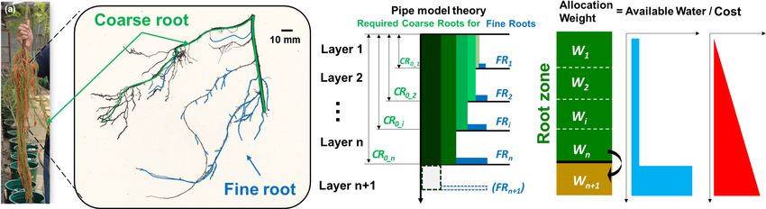
Figure 12. Evolution of the drying soil layers with stand age simulated by (a) the static rooting depth (S–D) and (b) the dynamic rooting
depth (D–D) approaches over a 50-year period at Yongshou, Loess Plateau. The triangles and squares are the respective observed upper and
lower boundaries adopted from Jia et al. (2017a). The abbreviations used in the figure are as follows: DSL-UB – the upper boundary of the
drying soil layer; DSL-LB – the lower boundary of the drying soil layer; DSL-SWC – the mean soil water content within the drying soil
layer; DSLT – the thickness of the drying soil layer.
the results section. The continuous development of the lower restoration practices in the Loess Plateau, for example, the
boundary of the drying soil layer implies that its recovery is “Grain for Green” project implemented in 1999.
critically difficult. This is because of the large thickness and
vast storage capacity of loess soil (Huang and Shao, 2019). 4.2 Outlooks of future work
Plants tend to develop more fine roots in the topsoil and use
more soil water due to lower costs but higher benefits, re- Roots develop beneath the ground, which is widely accepted
sulting in a more profitable adaptation strategy when expe- to be critically difficult to monitor; the deeper the soil depth,
riencing water stress. Exploration of water from wetter but the harder it is to sample (Maeght et al., 2013; Warren et al.,
deeper soil is also an adaption strategy when it is more prof- 2015; Fan et al., 2017). Observations of the rooting depths
itable, but deep roots might be more expensive to construct are rarely available for ready use, especially knowledge of
and maintain (Pierret et al., 2016; Germon et al., 2020). This the maximum rooting depth for vegetation in a region. Occa-
explains why the top 2.0 m soil was the most active zone of sionally, the limited data may provide a rough estimate; for
water uptake in this study. Depletion of topsoil always va- example, H. Li et al. (2019) and Wu et al. (2021) reported
cates the storage for infiltration, making it difficult for the some maximum rooting depths of apple trees and black lo-
rainfall to replenish the deeper dried soil layer or groundwa- cust of approximately 25.0 m (H. Li et al., 2019; Wu et al.,
ter (Turkeltaub et al., 2018). 2021). Mathematical simulation is a beneficial compensation
The occurrence and development of a drying soil layer sig- for field observations and can go far beyond its limitations,
nificantly impact the plant–water relationship and the local although its effectiveness relies on the actual data. The sim-
hydrological cycling in the Loess Plateau, where the combi- ulation can reproduce the dynamics of roots at very fine tem-
nation of deep loess soil and the semi-arid and arid climate poral and spatial resolutions, while in situ data are usually
prevails (Zhao et al., 2019). This might also be an issue in extremely rare. This study adopted in situ data at only a sin-
other regions with similar soil and climate conditions (Shao gle moment, as shown in Fig. 3. Fortunately, it was found
et al., 2018); in fact, this phenomenon has also been reported that the measurements fell within the variation range of the
elsewhere, such as in the Amazonia forest (Jipp et al., 1998) simulations over some time periods, which is understandable
and southern Australia dryland (Robinson et al., 2006), due from a statistical point of view. In situ data are believed to
to artificial afforestation. The occurrence of a persistent dry- remain an issue in the development and evaluation of root
ing soil layer not only degrades soil and vegetation but also approaches in the long term (Pierret et al., 2016).
negatively impacts ecosystem functions and services (Huang The simulation results indicated that the annual infiltra-
and Shao, 2019), such as the degeneration of the artificially tion amount from the static rooting depth approach was
planted trees (Jia et al., 2017a). The drying soil layer and 4.0 % higher than that of the dynamic rooting depth approach
the degraded artificial afforestation are believed to be mutu- (Fig. 10). In the field, no surface runoff was found during the
ally causative. The long-term simulation results also affirm years of observation at the study site at Yeheshan. The minor
the importance of monitoring both the long-term vegetation difference in the infiltration amount between these two root-
and soil water dynamics of artificial forests for ecosystem ing depth approaches was due to canopy interception. The
static rooting depth approach limits the roots to develop and
https://doi.org/10.5194/hess-26-17-2022 Hydrol. Earth Syst. Sci., 26, 17–34, 2022You can also read