An observation-based evaluation and ranking of historical Earth system model simulations in the northwest North Atlantic Ocean
←
→
Page content transcription
If your browser does not render page correctly, please read the page content below
Biogeosciences, 18, 1803–1822, 2021
https://doi.org/10.5194/bg-18-1803-2021
© Author(s) 2021. This work is distributed under
the Creative Commons Attribution 4.0 License.

An observation-based evaluation and ranking of historical Earth
system model simulations in the northwest North Atlantic Ocean
Arnaud Laurent1 , Katja Fennel1 , and Angela Kuhn2
1 Department     of Oceanography, Dalhousie University, Halifax, Nova Scotia, Canada
2 Scripps   Institution of Oceanography, UC San Diego, La Jolla, CA, USA

Correspondence: Arnaud Laurent (arnaud.laurent@dal.ca)

Received: 11 July 2020 – Discussion started: 17 July 2020
Revised: 9 January 2021 – Accepted: 25 January 2021 – Published: 16 March 2021

Abstract. Continental shelf regions in the ocean play an im-      indicates that only one ESM has good and consistent perfor-
portant role in the global cycling of carbon and nutrients, but   mance for all variables. An additional evaluation of the ESMs
their responses to global change are understudied. Global         along the regional model boundaries shows larger variabil-
Earth system models (ESMs), as essential tools for build-         ity but is generally consistent with the ranking on the shelf.
ing understanding of ocean biogeochemistry, are used exten-       Overall, 11 ESMs were deemed satisfactory for use in the
sively and routinely for projections of future climate states;    NWA, either directly or for regional downscaling.
however, their relatively coarse spatial resolution is likely
not appropriate for accurately representing the complex pat-
terns of circulation and elemental fluxes on the shelves along
ocean margins. Here, we compared 29 ESMs used in the In-          1   Introduction
tergovernmental Panel on Climate Change (IPCC)’s Assess-
ment Reports (ARs) 5 and 6 and a regional biogeochemical          Elemental fluxes along ocean margins, which are areas of
model for the northwest North Atlantic (NWA) shelf to as-         complex physical and biogeochemical interactions, are im-
sess their ability to reproduce surface observations of tem-      portant components of the global cycles of carbon (C) and
perature, salinity, nitrate and chlorophyll. The NWA region       nitrogen (N). For example, continental shelves host up to a
is biologically productive, influenced by the large-scale Gulf    third of oceanic primary production and over 40 % of carbon
Stream and Labrador Current systems and particularly sen-         burial in the ocean (Ducklow and McCallister, 2004; Muller-
sitive to climatically induced changes in large-scale circu-      Karger, 2005; Walsh, 1991). They also are important sites
lation. Most ESMs compare relatively poorly to observed           of sediment denitrification leading to a net removal of fixed
surface nitrate and chlorophyll and show differences with         nitrogen (Fennel et al., 2006; Seitzinger and Giblin, 1996).
observed surface temperature and salinity that suggest spa-       Many shelf regions are thought to be a significant sink for at-
tial mismatches in their large-scale current systems. Model-      mospheric CO2 (Cai et al., 2006; Chen et al., 2013; Laruelle
simulated nitrate and chlorophyll compare better with avail-      et al., 2018), including the eastern margin of North America
able observations in AR6 than in AR5, but none of the mod-        (Fennel et al., 2019, and references therein), although there
els perform equally well for all four parameters. The en-         are significant discrepancies in available estimates. Despite
semble means of all ESMs, and of the five best-performing         their importance, the response of ocean margins to climate
ESMs, strongly underestimate observed chlorophyll and ni-         change is understudied relative to the open ocean.
trate. The regional model has a much higher spatial reso-            Future projections of ocean biogeochemistry rely heav-
lution and reproduces the observations significantly better       ily on Earth system models (ESMs). These are state-of-the-
than any of the ESMs. It also simulates reasonably well ver-      art comprehensive representations of the major Earth system
tically resolved observations from gliders and bi-monthly         components (including atmosphere, ocean and land surface)
ship-based monitoring observations. A ranking of the ESMs         and are routinely used to perform climate scenario projec-
                                                                  tions. The spatial resolution of the CMIP-class ESMs typ-

Published by Copernicus Publications on behalf of the European Geosciences Union.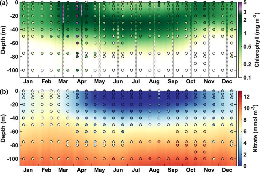
1804                  A. Laurent et al.: Evaluation of historical ESM simulations in the northwest North Atlantic Ocean

ically ranges from 0.5 to 2◦ and is too coarse to resolve         variability across models) or global assessments rather than
coastal ocean dynamics and interactions between shelf and         on regional model performance. However, ESMs that poorly
the open ocean (Anav et al., 2013; Bonan and Doney, 2018;         represent the dynamics of the NWA will affect the results of
Holt et al., 2017). This leads to uncertainty in future projec-   regional studies.
tions, not only for margin regions, and a global underestima-        Increased coastal model resolution can be achieved by
tion of the high primary productivity in coastal regions (Bopp    downscaling large-scale or global models, the so-called par-
et al., 2013; Schneider et al., 2008).                            ent models, to high-resolution regional models, the child
   Regional coupled circulation–biogeochemical models             models (see, e.g., Hermann et al., 2019; Holt et al., 2016;
have been developed at much higher spatial resolution. These      Laurent et al., 2018; Lavoie et al., 2020). For future pro-
regional models have been used to investigate biogeochemi-        jections, the obvious approach is to downscale ESMs. Since
cal processes along ocean margins (Fennel et al., 2006, 2013;     simulation of the fine-scale processes in the child model is
Lachkar and Gruber, 2011; Peña et al., 2019; Siedlecki et al.,    strongly influenced by the parent model, it is important to
2015; Zhang et al., 2020) and project future states resulting     assess the skill of ESMs in reproducing historical observa-
from climate change (Gruber et al., 2012; Hermann et al.,         tions prior to using them for downscaled future projections.
2016; Holt et al., 2016; Laurent et al., 2018). The regional      Rickard et al. (2016) ranked ESMs based on their misfit with
models allow for the temporal and spatial resolution neces-       regional observations around New Zealand in order to dis-
sary to resolve mesoscale processes and can be regionally         card models with significant errors and determine an en-
calibrated (e.g., Kuhn and Fennel, 2019; Mattern and Ed-          semble of “best” models that can be used to study regional
wards, 2017). However, the dynamics of a regional model           climate projections, either directly or indirectly through re-
is strongly determined by information imposed along the           gional downscaling. Here, we take a similar approach.
model’s open lateral boundaries, typically derived from a            Our main objective is to assess the performance of a num-
larger-scale model, reanalysis product or observation-based       ber of available ESMs in reproducing present conditions
climatology. For future climate simulations, a regional model     on the NWA shelf in contrast to a high-resolution regional
requires boundary information from future projections of          model. This is important information for users of histori-
large-scale models or ESMs.                                       cal and future projections in the region. Additionally, we
   The northwest North Atlantic (NWA), located at the con-        assess ESM performance along the boundaries of the re-
fluence of the subtropical and subpolar gyres, is particularly    gional model. This information is necessary when downscal-
challenging to global ocean circulation models and highly         ing with a regional model. More specifically, we compare 29
sensitive to climate-induced modifications of the large-scale     ESMs used in the two most recent Intergovernmental Panel
circulation, which are thought to be responsible for a multi-     on Climate Change (IPCC) Assessment Reports (ARs) as
decadal deoxygenation trend in the region (Claret et al.,         part of the fifth phase of the Coupled Model Intercompar-
2018; Gilbert et al., 2005, 2010). While the CMIP models          ison Project (CMIP5; Taylor et al., 2012) and its currently
reasonably describe the large-scale climatological features       ongoing successor, CMIP6 (Eyring et al., 2016). We carry
of ocean physics in the NWA, the detailed current structure       out a systematic and quantitative assessment and ranking by
is poorly represented due to a mismatch in the location of        comparing the CMIP5 and CMIP6 models against observed
the subtropical and subpolar gyres (Loder et al., 2015). The      surface temperature, salinity, chlorophyll and nitrate and per-
Gulf Stream usually extends too far north, and the branch of      form the same comparisons for a regional biogeochemical
the Labrador Current flowing southwest along the shelf edge       model. The latter is the Atlantic Canada Model (ACM; Bren-
tends to be missing (Lavoie et al., 2019; Loder et al., 2015).    nan et al., 2016; Rutherford and Fennel, 2018) with biogeo-
This leads to a warm bias in the NWA, a common feature            chemistry (Bianucci et al., 2016; Kuhn and Fennel, 2019)
among coarse-resolution ESMs (Saba et al., 2016). The ab-         and is intended for regional downscaling of ESM simula-
sence of the shelf-break current significantly impacts cross-     tions in order to generate high-resolution future projections.
shelf exchange with much larger shelf water residence times       For all models, we present statistical metrics based on the
in a high-resolution regional model (Rutherford and Fennel,       mismatch of each model with climatological surface obser-
2018) compared to estimates from a global model (Bourgeois        vations of temperature, salinity, nitrate and chlorophyll and
et al., 2016). These discrepancies have been attributed to the    a ranking based on these metrics. The regional model is fur-
coarse resolution of the global models (Lavoie et al., 2019;      ther evaluated against in situ measurements, including high-
Loder et al., 2015; Rutherford and Fennel, 2018; Saba et al.,     resolution cross-shelf glider transects. The comparison pro-
2016). Despite these issues, CMIP historical simulations and      vides an overview of ESM performance in the NWA and
future projections have been used to characterize biological      shows sufficient confidence for only a third of the ESMs.
responses to climate change in the NWA (e.g., Bryndum-            The regional model clearly outperformed all the global mod-
Buchholz et al., 2020a; Greenan et al., 2019; Lavoie et al.,      els, and regional downscaling using single-ESM forcing (as
2019; Stortini et al., 2015; Wilson et al., 2019; Wilson and      opposed to an ensemble) is recommended.
Lotze, 2019). ESM selection in these regional studies is ei-
ther qualitative or based on either scenario outcomes (e.g.,

Biogeosciences, 18, 1803–1822, 2021                                                 https://doi.org/10.5194/bg-18-1803-2021

A. Laurent et al.: Evaluation of historical ESM simulations in the northwest North Atlantic Ocean                                         1805

Figure 1. Study area indicating the three averaging zones, the lim-      Figure 2. Schematic of the biogeochemical model used in ROMS.
its of the Regional Ocean Modeling System (ROMS) grid and the            The state variables are small phytoplankton (PS ) and chlorophyll
location of the Halifax Line stations (squares) used in the analysis.    (ChlS ), large phytoplankton (PL ) and chlorophyll (ChlL ), small
The white star is Station 2 and the gray lines are the gliders’ track.   zooplankton (ZS ), large zooplankton (ZL ), slow-sinking small de-
                                                                         tritus (DS ), fast-sinking large detritus (DL ), nitrate (NO3 ) and am-
                                                                         monium (NH4 ). Dashed lines indicate sinking. Black dots represent
2     Material and methods                                               the connections between paths.

2.1     Models

2.1.1    Global models                                                   Haidvogel et al., 2008) for the NWA, nested within the larger
                                                                         ocean–ice model of Urrego-Blanco and Sheng (2012) that
The CMIP5 and CMIP6 framework provides state-of-the-art                  includes the Gulf of Maine, Scotian Shelf and Grand Banks
climate model datasets from the previous (AR5) and current               (Fig. 1). The coupled physical–biogeochemical model has 30
(AR6) IPCC Assessment Reports (Eyring et al., 2016; Taylor               vertical layers and an average horizontal resolution of 9.5 km
et al., 2012). Of all the ESMs, those that include ocean bio-            on the shelf (Table 1). Detailed descriptions and physical
geochemistry with monthly outputs of surface temperature,                model validation are presented in Brennan et al. (2016) and
salinity, chlorophyll and nitrate were included in our com-              Rutherford and Fennel (2018). The biogeochemical model
parison. A total of 29 such ESMs were available (Table 1):               is based on Fennel et al. (2006, 2008) but was expanded by
17 from CMIP5 (models 2–18) and 12 from CMIP6 (models                    splitting phytoplankton and zooplankton state variables into
19–30). These models vary in their horizontal and vertical               size-based functional groups, i.e., nano-microphytoplankton
resolution and include a total of 13 different ocean biogeo-             and micro-mesozooplankton. The model was also modi-
chemical models of varying levels of complexity (Table 1                 fied by including temperature-dependent biological rates for
and references therein).                                                 nutrient uptake, phytoplankton and zooplankton mortality,
   We accessed the historical simulations which were forced              grazing and zooplankton egestion and excretion (see Supple-
by observed atmospheric composition and land cover                       ment text). The model has 10 state variables: nitrate, ammo-
changes over the period ∼ 1850–2005 (CMIP5) and ∼ 1850–                  nium and two size classes each for phytoplankton, chloro-
2014 (CMIP6). Monthly spatially resolved climatologies of                phyll, zooplankton and detritus (Fig. 2). This ecosystem
surface chlorophyll, nitrate, temperature and salinity were              structure of intermediate complexity is similar to the model
calculated over 30 years (1975–2005) from each ESM his-                  of Aumont et al. (2015), which is used in six of the ESMs in-
torical simulation.                                                      cluded in our study. Model parameters were optimized by
                                                                         Kuhn (2017) and are listed in Supplement Table S1. The
2.1.2    Regional model                                                  model description and equations are available in the Supple-
                                                                         ment.
The ACM is a high-resolution regional configuration of                      Initial and open boundary conditions for nitrate (NO3 )
the Regional Ocean Modeling System (ROMS, version 3.5;                   were defined from a monthly climatology (Kuhn, 2017)

https://doi.org/10.5194/bg-18-1803-2021                                                            Biogeosciences, 18, 1803–1822, 2021
1806 A. Laurent et al.: Evaluation of historical ESM simulations in the northwest North Atlantic Ocean
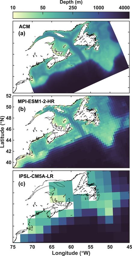
300 times more than the lowest-resolution ESM. Among the
ESMs, the highest resolution is achieved by models 16 and
28, which share the same grid. These two have more than
twice the number of horizontal grid cells compared to the
next-highest-resolution models (3, 18, 20–21). The lowest-
resolution ESMs are models 3 and 12–14 with only 26 hori-
zontal grid cells within the NWA shelf, resulting in a coarse
representation, particularly in the Scotian Shelf (SS) region.
The median number of grid cells in the NWA shelf region is
72 and 102 for the CMIP5 and CMIP6 models, respectively,
compared to 6875 in the ACM.
2.1.4 Observations
Four types of observations were used in the model intercom-
parison: (1) satellite surface chlorophyll observations from
the Sea-viewing Wide Field-of-view Sensor (SeaWiFS) as
8 d averaged maps at 1/12◦ resolution (1999–2010, SeaWiFS
2018), (2) surface nitrate from the World Ocean Atlas 2013
(WOA; Garcia et al., 2014) at 1◦ resolution, (3) daily surface
temperature from the Operational SST and Sea Ice Analysis
(OSTIA) system (Donlon et al., 2012) at 1/20◦ resolution
(2006–2016; UK Met Office 2005) and (4) surface salin-
ity from the WOA at 1/4◦ resolution (Zweng et al., 2013).
Monthly climatologies were calculated for each of these.
In addition, the regional model was validated using high-
resolution in situ observations along the Halifax Line (Fig. 1)
from the Atlantic Zone Monitoring Program (AZMP, 2000–
2014) and glider transects between 2011 and 2016 (Ross
et al., 2017). To enable a quantitative comparison between
the glider and ACM data (Table 3), we spatially interpo-
lated both datasets onto a transect following the Halifax Line
(black line in Fig. 1). Glider missions were seasonal, and
therefore both glider and AZMP transects data were season-
ally averaged. For each mission, data were extracted at Sta-
tion 2 to produce a monthly climatology.
Figure 3. Bathymetry of the regional model (a), the highest-
resolution ESM (b) and lowest-resolution ESM (c). 2.1.5 Comparison metrics
For comparison with the observations, each model was
based on in situ observations and the World Ocean At- mapped onto the SeaWiFS, WOA and OSTIA grids using a
las 2009 (Garcia et al., 2010). Other biological variables were nearest-neighbor interpolation. Since some areas, such as the
set to 0.1 mmol N m−3 with a phytoplankton-to-chlorophyll nearshore area and the Bay of Fundy, are covered by only
ratio of 0.76 mmol N (mg Chl)−1 (Bianucci et al., 2016). The a few models, grid cells that are active in less than 85 %
model was initialized on 1 January 1999 and run through of all models were excluded from the analysis to avoid bi-
31 December 2014. The first year was considered spin-up. ases. In the low-resolution WOA climatology, the months of
Monthly climatologies of surface chlorophyll, nitrate and November–January were excluded because poor data avail-
temperature were calculated for comparison with the ESMs. ability in these months resulted in unrealistic patterns.
Three zones were defined for a high-level comparison with
2.1.3 Model resolution the observations on the shelf: the Gulf of Maine (GoM),
SS and Grand Banks (GB) (Fig. 1). Subsequently, the term
The 30 models differ dramatically in their horizontal reso- “NWA shelf” refers to the region covered by all three zones
lution and do not evenly cover the three regions of interest (GoM, SS and GB). An additional zone was also defined for
(Fig. 3, Table 1). The regional ACM has a much higher reso- a high-level comparison with the observations along the open
lution than any of the ESMs with about 16 times more hori- boundaries of the ACM.
zontal grid cells than the highest-resolution ESM and almost
Biogeosciences, 18, 1803–1822, 2021 https://doi.org/10.5194/bg-18-1803-2021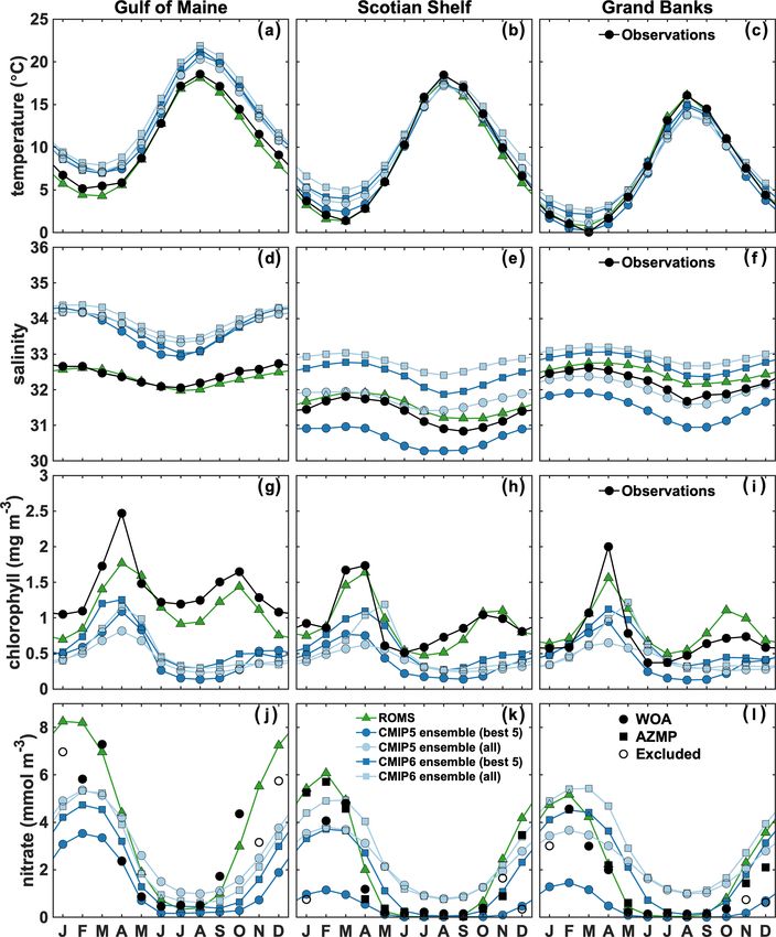
A. Laurent et al.: Evaluation of historical ESM simulations in the northwest North Atlantic Ocean                                          1807

Table 1. Information about the regional model and the 29 ESM models. For the CMIP5 models (2–18) the r1i1p1 ensemble was used. For
the CMIP6 model (19–30) the r1i1p1f1 ensemble was used on the native grid when available, except for CNRM-ESM2-1, MIROC-ES2L
and UKESM1-0-LL (r1i1p1f2), GFDL-ESM4 and NorESM2-LM (regridded), and GISS-E2-1-G (r101i1p1f1). The filled circles and open
squares indicate the models that are part of the inner and outer ensembles, respectively. The table provides the number of grid cells in
the GoM, SS and GB regions, the average grid resolution on the shelf (1lon × 1lat, degrees) and the number of vertical levels (N). Note
that the IPSL-CM5 models share the same ocean component with higher resolution atmospheric component in the MR version. Similarly,
MPI-ESM-MR and MPI-ESM1-2-HR share the same ocean component with higher resolution atmospheric component in the HR version.

   Name              ID    ∈   GoM       SS    GB    1lon ×1lat     N     Ocean BGC        References
   ACM                1    –   1780    1366   3729    0.06 × 0.09   30    BIO_FENNEL       Brennan et al. (2016), Fennel et al. (2006)
   CanESM2            2          11     14     29      1.4 × 0.9   40    CMOC             Arora et al. (2011), Christian et al. (2010)
   CESM1-BGC          3          41     33     91      1.1 × 0.4   60    BEC              Lindsay et al. (2014), Moore et al. (2013)
   CMCC-CESM          4           8      5     13       2 × 1.25   30    PELAGOS          Vichi et al. (2007a, b, 2011)
   CNRM-CM5           5          27     20     55       1 × 0.62   42    PISCES           Aumont and Bopp (2006), Voldoire et al. (2013)
   GFDL-ESM2-G        6    •
                                  20     15     39         1×1      50    TOPAZ2           Dunne et al. (2012, 2013), Dunne (2013)
   GFDL-ESM2-M        7
   GISS-E2-H-CC       8          19     14     39          1×1     26
                                                                          NOBM             Romanou et al. (2013), Schmidt et al. (2014)
   GISS-E2-R-CC       9          15     12     29       1.25 × 1   32
   HadGEM2-CC        10    •
                                  18     15     39         1×1      40    Diat-HadOCC      Collins et al. (2011), Palmer and Totterdell (2001)
   HadGEM2-ES        11
   IPSL-CM5A-LR      12    •
   IPSL-CM5A-MR      13    •       8      5     13       2 × 1.25   31    PISCES           Aumont and Bopp (2006), Dufresne et al. (2013)
   IPSL-CM5B-LR      14
   MPI-ESM-LR        15          23     23     73      0.8 × 0.5   47
                                                                          HAMOCC 5.2       Giorgetta et al. (2013), Ilyina et al. (2013)
   MPI-ESM-MR        16    •     136     87    193      0.4 × 0.3   95
   MRI-ESM1          17          40     29     80        1 × 0.5   50    MRI.COM3         Adachi et al. (2013)
   NorESM1-ME        18          41     33     91       1 × 0.43   53    HAMOCC 5.1       Tjiputra et al. (2013)
   CanESM5           19          27     20     55       1 × 0.62   45    CMOC             Swart et al. (2019)
   CESM2             20
                                  41     33     91       1 × 0.43   60    MARBL            Danabasoglu et al. (2020)
   CESM2-WACCM       21
   CNRM-ESM2-1       22    •      27     20     55       1 × 0.62   75    PISCES           Aumont et al. (2015), Séférian et al. (2019)
   GFDL-ESM4         23          20     15     39         1×1      75    COBALTv2         Stock et al. (2020)
   GISS-E2-1-G       24
                                  15     12     29       1.25 × 1   40    NOBM             Rousseaux and Gregg (2015)
   GISS-E2-1-G-CC    25    •
   IPSL-CM6A-LR      26    •      27     20     55       1 × 0.62   75    PISCES           Aumont et al. (2015), Boucher et al. (2020)
   MIROC-ES2L        27    •      20     18     43       1 × 0.77   62    OECO2            Hajima et al. (2020)
   MPI-ESM1-2-HR     28    •     136     87    193      0.4 × 0.3   95    HAMOCC           Müller et al. (2018)
   NorESM2-LM        29          25     20     57        1 × 0.6   70    HAMOCC           Müller et al. (2018)
   UKESM1-0-LL       30    •      27     20     55       1 × 0.62   75    MEDUSA2          Sellar et al. (2019), Yool et al. (2013)

   Following the method of Rickard et al. (2016), a score S              the model (y), such that
was calculated for each model variable, υ (i.e., surface tem-                      v
                                                                                   u n
perature, chlorophyll and nitrate), for each month, t, in the                      u1 X
climatology as the sum of the centered root mean square dif-             S(t, υ) = t       ((xi (t, υ) − x(t, υ)) − (yi (t, υ) − y(t, υ)))2
                                                                                     n i=1
ference (RMSD) and bias between the observations (x) and
                                                                                       n
                                                                                    1 X
                                                                                +         xi (t, υ) − y i (t, υ) ,
                                                                                    n i=1

                                                                         where the index i refers to a grid cell and n is the total num-
                                                                         ber of grid cells within the NWA shelf. The lower the score,

https://doi.org/10.5194/bg-18-1803-2021                                                           Biogeosciences, 18, 1803–1822, 2021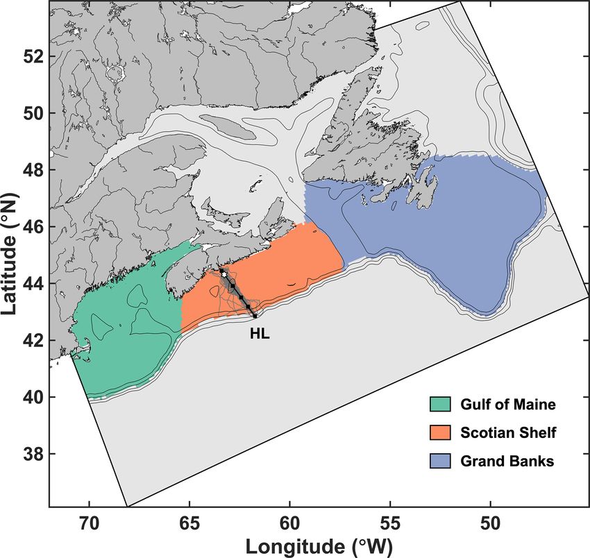
1808                  A. Laurent et al.: Evaluation of historical ESM simulations in the northwest North Atlantic Ocean

the better the match between model and observations. Annual
mean scores S(υ) were calculated for each model variable by
averaging over t. For each variable, the models were ranked
based on their annual mean score. The overall rank was de-
termined by ranking models by the averages of their ranks
for surface temperature, salinity, chlorophyll and nitrate (R).
For models with equal averages, the ranking was determined
by the average of chlorophyll and nitrate ranks (R bio ).
   To facilitate the comparison with observations, the ESMs
were grouped into CMIP5 and CMIP6 and the ensemble
means of all models and of the five highest-ranked models
were calculated for each group.

3     Results

Models and model ensembles are first compared with obser-
vations to assess their ability to reproduce the annual cycles
of surface temperature, salinity, chlorophyll and nitrate in the
NWA region. Error statistics are then analyzed to understand
how the models deviate from each observed variable and sub-
sequently used to calculate the scores and then rank the mod-
els. Finally, additional, high-resolution comparisons between
models and observations are presented to further assess the
regional model’s performance.
                                                                    Figure 4. Observed, ROMS and ensemble means’ area-averaged
3.1    Model–data comparisons                                       surface temperature (a–c), salinity (d–f), chlorophyll (g–i) and ni-
                                                                    trate (j–l) in the NWA shelf regions. November–January WOA ni-
First, we compare the spatially averaged climatological sur-        trate data are excluded (open circles). Model comparison with ob-
face temperature (Figs. 4 and 5a–c), salinity (Figs. 4 and 5d–      servations in the Gulf of Maine is therefore only available from
f), chlorophyll (Figs. 4 and 5g–i) and nitrate (Figs. 4 and 5j–l)   February to October. For the Scotian Shelf and Grand Banks, ad-
in our three regions of interest. The ESMs reasonably repro-        ditional AZMP data are available. In the case of multiple observa-
duce the annual cycle of surface temperature, but the annual        tions, the data are monthly averaged.
cycles of salinity, chlorophyll and nitrate are not simulated
well in any of them (see Supplement Figs. S1–S5) and the
range of simulated salinity and biological properties is large.     and magnitude of the spring and fall blooms (Figs. 5g–i, S1–
   Temperature is relatively consistent between model en-           S5g–i). Standard deviations for the magnitude of the spring
sembles (Fig. 4a–c) but with large variability between mod-         bloom are large among ESMs in the three zones (SD of
els (Fig. 5a–c). An annual, positive bias occurs in the GoM         0.6, 0.81 and 0.83 mg m−3 in GoM, SS and GB, respec-
(bias of +2.30 ◦ C; Fig. 4a), whereas temperatures are over-        tively). The maxima of the spring bloom also vary signif-
estimated in winter (December–February) on the SS and GB            icantly in time among the models, with a standard devia-
(bias of +1.95 and +0.94 ◦ C, respectively; Fig. 4a–c) and          tion among ESMs for the time of maxima of the bloom
underestimated in summer (June–August) on GB (−1.53 ◦ C;            of about 1.5 months (SD of 1.15, 1.59 and 1.62 months in
Fig. 4f).                                                           GoM, SS and GB, respectively). Most models in the CMIP5
   The range of simulated surface salinity is large (Fig. 4d–       group do not simulate a fall bloom; hence, none are present
f). Most models overestimate salinity in the GoM (bias of           in the ESM ensemble mean, but rather there is a fall–winter
+1.46; Fig. 4d). The mismatch is large on the SS and GB             increase in chlorophyll concentrations. Among the CMIP6
but not consistent among models, except for an annual, pos-         group, only models 23–25 generate a fall bloom (see Sup-
itive bias in CMIP6 models (bias of +1.42 and +0.76, re-            plement Figs. S4–S5g–i). Overall, the ESMs underestimate
spectively; Fig. 4e–f). In the two latter regions, the biases in    annual surface chlorophyll concentrations (bias of −0.94,
CMIP5 models compensate each other, resulting in an en-             −0.50 and −0.29 mg m−3 for GoM, SS and GB, respec-
semble mean close to the observations.                              tively; Fig. 4g–i). The chlorophyll bias is about 20 % smaller
   For surface chlorophyll, there is a large discrepancy be-        in the CMIP6 group compared to CMIP5.
tween the model ensembles and observations (Fig. 4g–i).                There are also large discrepancies between the model en-
Inter-model differences are largest for the time of maxima          sembles and observations for nitrate (Fig. 4j–l), particularly

Biogeosciences, 18, 1803–1822, 2021                                                     https://doi.org/10.5194/bg-18-1803-2021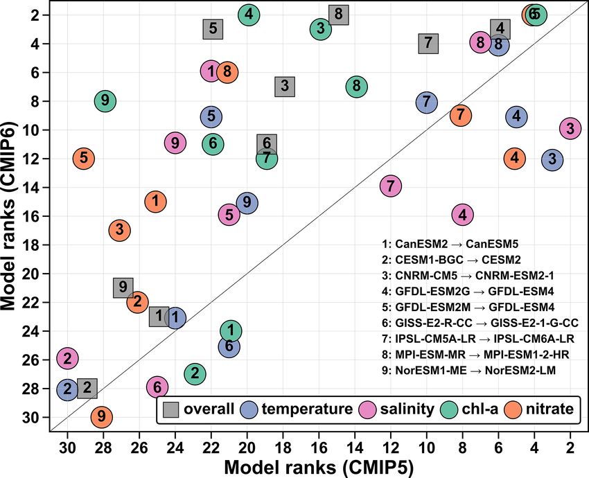
A. Laurent et al.: Evaluation of historical ESM simulations in the northwest North Atlantic Ocean                                 1809

                                                                           The regional ACM well reproduces the annual cycle of
                                                                        surface temperature (Fig. 4a–c), salinity (Fig. 4d–f), chloro-
                                                                        phyll (Fig. 4g–i) and nitrate (Fig. 4j–l) in the three regions.
                                                                        The model correctly simulates the overall magnitude of tem-
                                                                        perature and chlorophyll biomass, the timing of the max-
                                                                        ima of spring and fall blooms and the latitudinal variations
                                                                        in temperature, salinity, chlorophyll and nitrate, although the
                                                                        magnitude of the spring bloom in the GoM and GB regions
                                                                        is underestimated. Late summer surface salinity is slightly
                                                                        overestimated on the SS and GB.

                                                                        3.2   Model statistics

                                                                        Error statistics, i.e., RMSD and bias, are now analyzed and
                                                                        used to calculate the model scores. The distribution and rela-
                                                                        tionships between scores are explored and then the ranks are
                                                                        calculated.
                                                                           Except for the relationship between temperature and salin-
                                                                        ity RMSD (r = 0.82, p < 0.001), the RMSDs between the
                                                                        spatially averaged climatological observations and models
                                                                        are not consistent between variables, as indicated by the in-
                                                                        creasing temperature RMSD in Fig. 6. However, tempera-
                                                                        ture and chlorophyll RMSD are weakly correlated (r = 0.50,
                                                                        p = 0.005). For temperature and salinity, models 3, 20–21
                                                                        and 24–25 have the largest discrepancy with observations,
Figure 5. Observed (black dots) and best ESMs’ area-averaged sur-       and some clearly represent the annual cycle better than oth-
face temperature (a–c), salinity (d–f), chlorophyll (g–i) and nitrate   ers. The best models for temperature (5–6, 14, 16 and 28)
(j–l) in the three NWA shelf regions. The colored circles and squares   do not always match the best for salinity (5, 16, 27–28, 30).
indicate the CMIP5 and CMIP6 models, respectively. November–            For chlorophyll, the largest discrepancies with observations
January WOA nitrate data are excluded (open circles). Model com-        are in models 4, 8, 14 and 19–21, but overall chlorophyll
parison with observations in the Gulf of Maine is therefore only        RMSDs are relatively large and homogeneous, except for a
available from February to October. For the Scotian Shelf and Grand     few models that have lower RMSD (e.g., models 22–23). In-
Banks, additional AZMP data are available. In the case of multiple      terestingly, the magnitude of the spring bloom in model 18
observations, the data are monthly averaged.
                                                                        (CMIP5 group) is somewhat close to the observations. How-
                                                                        ever, the time shift of the bloom (May–June) results in a
                                                                        poor agreement with observations. The mismatch between
in the CMIP5 group. The variability in nitrate concentra-
                                                                        observed and simulated nitrate is much higher for models
tions among the ESMs is also large (SD of 2.80 mmol m−3 )
                                                                        5, 7, 18 and 29, and some models are much better at rep-
but smaller by 29 % in the CMIP6 group. Most of the
                                                                        resenting the observed annual cycle (Fig. 6), as indicated
models reproduce the seasonal variability of surface nitrate
                                                                        by the lower RMSD. The RMSDs of the ACM are about a
(Figs. 5j–l, S1–S5j–l); however, the CMIP5 models tend
                                                                        third of the average RMSD of the ESMs for both chlorophyll
to underestimate fall–winter concentrations (winter bias of
                                                                        (ESM RMSDs are a factor of 2.0–4.1 larger than those of
−1.28 mmol m−3 ), whereas the CMIP6 model group per-
                                                                        the ACM) and nitrate (factor of 1.4–11.4), a quarter for tem-
forms better but with some mismatches in the timing of the
                                                                        perature (factor of 1.1–10.4) and 13 % for salinity (factor of
seasonal changes (spring, fall). Note that since November–
                                                                        1.3–15.5).
January nitrate WOA observations were excluded from the
                                                                           Model scores (see Sect. 2.3) represent the spatial and tem-
analysis (see Sect. 2.1.5), winter observations are only avail-
                                                                        poral mismatch within the NWA shelf region (Fig. 7). In
able in February in the Gulf of Maine and in December and
                                                                        general, the scores provide similar results to the RMSDs in
January in Grand Banks. A few models markedly overesti-
                                                                        Fig. 6, although groups tend to emerge from the score calcu-
mate surface nitrate concentrations in the NWA shelf regions
                                                                        lation. As observed previously in Fig. 6, the scores of ESMs
(see Figs. S1, S3–5), including within the CMIP6 group. Fig-
                                                                        have a much larger range of variability for temperature (1.5–
ures S6–S9 provide an illustration of the model variability for
                                                                        7.8), salinity (0.5–4.2) and nitrate (1.4–13.2) than for chloro-
chlorophyll and nitrate in March (Figs. S6 and S7) and Octo-
                                                                        phyll (0.81–1.42) due to the large mismatch observed with
ber (Figs. S8 and S9), i.e., around the time of the spring and
                                                                        a few models (Figs. 7, S1–S5). For temperature, four of the
fall blooms, respectively.
                                                                        six poorest (largest) scores (>4.5) are in the CMIP6 group.

https://doi.org/10.5194/bg-18-1803-2021                                                          Biogeosciences, 18, 1803–1822, 2021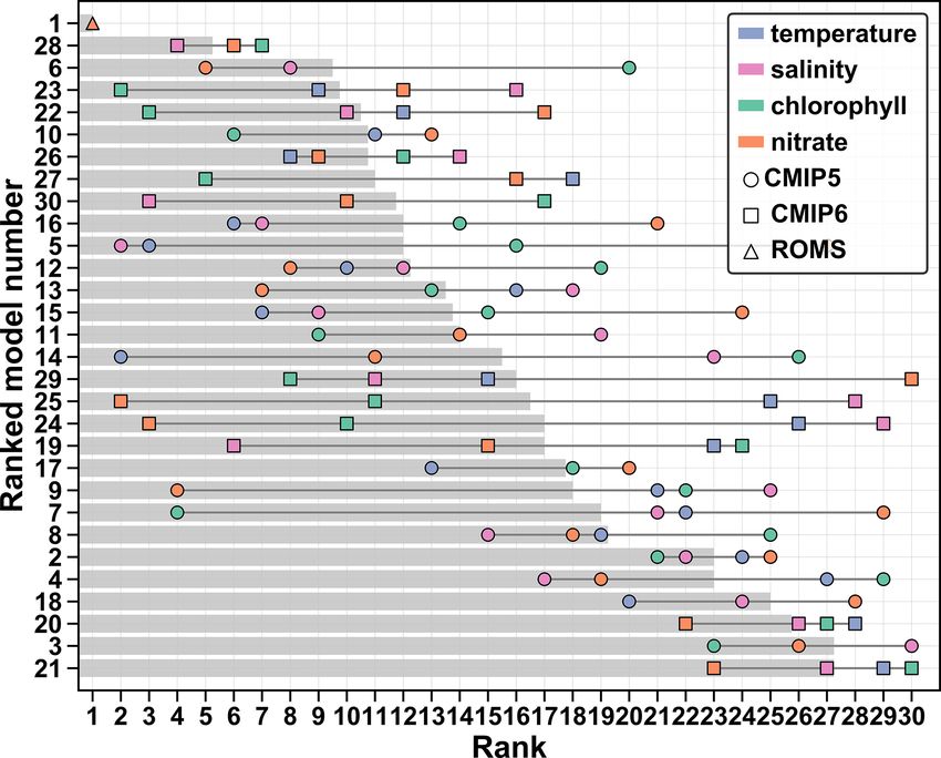
1810                  A. Laurent et al.: Evaluation of historical ESM simulations in the northwest North Atlantic Ocean

Figure 6. Root mean square difference between monthly, regionally averaged observations and models. Model numbers refer to the IDs in
Table 1.

They all markedly overestimate temperature, especially in            but among the best scores for temperature and salinity. In
the GoM (see Figs. S1, S4–S5), except for model 4, which             fact, only models 3 and 18 have poor scores for all variables.
underestimates temperature in SS and GB. The other mod-              Similarly, models 24 and 25 have the best scores for chloro-
els also have the poorest scores with respect to salinity. They      phyll but are among the worst for temperature and salinity.
all largely overestimate salinity in the three regions and are       On average, models have worse scores in the GoM (3.99,
clearly outliers with respect to their CMIP category. The            2.49, 1.73, 3.15) than on the SS (3.36, 2.35, 0.94, 2.22) and
range of variability in chlorophyll scores did not reduce from       GB (2.53, 1.41, 0.72, 2.47) for temperature, salinity, chloro-
CMIP5 to CMIP6 and given the relatively low scores of a              phyll and nitrate, respectively.
few CMIP6 models (i.e., 22 and 23), the range is larger in              Overall, four groups emerge on the chlorophyll–nitrate
the CMIP6 group (0.8–1.4; Fig. 7c) than in the CMIP5 group           space in Fig. 7. This grouping is somewhat arbitrary but pro-
(1–1.4; Fig. 7a). With the exception of model 29, which has          vides a “biological” focus on model performance that can
a very poor (high) score for nitrate, the range of variability       be related to the biological ranking (R bio ) in Table 2. It also
in nitrate is reduced in the CMIP6 group. In total, five mod-        follows the general ranking presented in Fig. 8, with a few
els (3, 5, 7, 18, 29) have very poor scores for nitrate (>4),        exceptions. Group A includes 11 of the 14 best models (five
strongly overestimating surface nitrate, except for model 3          for CMIP5 and six for CMIP6), except for models 9 and 24–
in the Gulf of Maine (see Fig. S1j–l). The remaining models          25 whose rankings are degraded due to poor representation of
have more homogeneous nitrate scores (Fig. 7) with the best          temperature and salinity. Within the 14 best models, the three
(lowest) scores in models 25, 24, 9 and 6 (Table 2). Models          models that are not included in Group A are models 5 and
that underestimate nitrate (2, 8, 14 and 19; see Figs. S1–S4)        15–16, which have intermediate to poor nitrate scores but are
have a better score because they match the low nitrate obser-        among the best models for temperature and salinity. Group B
vations in late spring–summer (Table 2). Overall, ACM has            includes four intermediate-score models with respect to biol-
the best scores, S(υ), for temperature (1.14), salinity (0.48),      ogy (15, 16, 17, 2). Group C includes the eight models with
chlorophyll (0.64) and nitrate (1.27).                               poor chlorophyll scores (five from CMIP5 and three from
   Among the four variables, and including the regional              CMIP6) and Group D the five models with poor nitrate scores
model, we found a correlation between the scores of tem-             (four from CMIP5 and one from CMIP6). Most of the models
perature and salinity (r = 0.74, p < 0.001), as well as weak         with poor scores for temperature and/or salinity are included
correlations between chlorophyll and temperature (r = 0.53,          in Group C, i.e., with the poor chlorophyll scores.
p = 0.0025) or salinity (r = 0.42, p = 0.02). There were                The overall model ranking (average of temperature, salin-
no correlations between nitrate and chlorophyll (r = 0.03,           ity, chlorophyll and nitrate ranks) indicates the gap between
p = 0.86, r = 0.53, p = 0.0025) and nitrate and temperature          ACM and ESMs, as well as within ESMs (Fig. 8). As ex-
(r = 0.05, p = 0.78) or salinity (r = 0.003, p = 0.99). As           pected, ACM ranks first, following the best scores for both
can be seen in Fig. 6, the ESMs with a poor representation           chlorophyll and nitrate. The gap between ACM and model
of nitrate are not necessarily performing poorly with respect        28 (ESM with best R and R bio ; Table 2) indicates that none
to the other variables. Model 7, for instance, has the poor-         of the ESMs perform best for all fields, especially for both
est score for nitrate and a relatively poor score for tempera-       chlorophyll and nitrate. This is also shown by the large range
ture and salinity but the best score of the CMIP5 group for          in individual ranks (dark gray lines in Fig. 8) in most models.
chlorophyll (Fig. 7a). Model 5 has a poor score for nitrate          Group A includes the eight best-ranking models: two from

Biogeosciences, 18, 1803–1822, 2021                                                     https://doi.org/10.5194/bg-18-1803-2021

A. Laurent et al.: Evaluation of historical ESM simulations in the northwest North Atlantic Ocean                                      1811

Figure 7. Model scores for surface chlorophyll (x axis), nitrate (y axis) and temperature (color scale) for the CMIP5 group (a), the CMIP6
group (b) and the regional model (triangles). Salinity and temperature scores are compared in panel (c). The gray ellipsoids indicate the
groups A–D (see text) and are the same in panels (a) and (b).

Table 2. Annual model scores and ranking. R represents the multivariable mean ranking and R bio the chlorophyll and nitrate mean ranking.
The final rank is provided in the right column. The bold values in the overall rank indicate a possible overestimation of the rank due to low
nitrate concentrations (Figs. S1–S5j–l).

          Ranked models                              Scores                                                Ranks
 Name                  ID    CMIP      Temp.    Salinity   Chl a     NO3      Temp.    Salinity   Chl a     NO3       R    R bio    Overall
 ACM                    1         –     1.14        0.48      0.64    1.27        1           1        1       1     1.0     1.0          1
 MPI-ESM1-2-HR         28         6     2.05        0.73      1.03    1.75        4           4        7       6     5.3     6.5          2
 GFDL-ESM2G             6         5     2.12        1.33      1.17    1.67        5           8       20       5     9.5    12.5          3
 GFDL-ESM4             23         6     2.49        2.10      0.81    2.10        9          16        2      12     9.8     7.0          4
 CNRM-ESM2-1           22         6     2.74        1.39      0.90    2.21       12          10        3      17    10.5    10.0          5
 HadGEM2-CC            10         5     2.58        2.02      1.02    2.11       11          13        6      13    10.8     9.5          6
 IPSL-CM6A-LR          26         6     2.47        2.03      1.09    1.94        8          14       12       9    10.8    10.5          7
 MIROC-ES2L            27         6     3.14        0.92      1.02    2.17       18           5        5      16    11.0    10.5          8
 UKESM1-0-LL           30         6     3.08        0.67      1.15    1.96       17           3       17      10    11.8    13.5          9
 CNRM-CM5               5         5     1.78        0.53      1.11    6.54        3           2       16      27    12.0    21.5         10
 MPI-ESM-MR            16         5     2.14        1.22      1.09    2.57        6           7       14      21    12.0    17.5         11
 IPSL-CM5A-LR          12         5     2.52        2.00      1.17    1.91       10          12       19       8    12.3    13.5         12
 IPSL-CM5A-MR          13         5     3.07        2.37      1.09    1.80       16          18       13       7    13.5    10.0         13
 MPI-ESM-LR            15         5     2.38        1.37      1.10    3.12        7           9       15      24    13.8    19.5         14
 HadGEM2-ES            11         5     2.90        2.50      1.06    2.12       14          19        9      14    14.0    11.5         15
 IPSL-CM5B-LR          14         5     1.51        2.64      1.36    2.03        2          23       26      11    15.5    18.5         16
 NorESM2-LM            29         6     2.95        1.81      1.05   13.23       15          11        8      30    16.0    19.0         17
 GISS-E2-1-G-CC        25         6     4.66        3.77      1.08    1.44       25          28       11       2    16.5     6.5         18
 CanESM5               19         6     4.05        1.18      1.35    2.16       23           6       24      15    17.0    19.5         19
 GISS-E2-1-G           24         6     5.00        3.89      1.08    1.47       26          29       10       3    17.0     6.5         20
 MRI-ESM1              17         5     2.78        2.63      1.15    2.53       13          20       18      20    17.8    19.5         21
 GISS-E2-R-CC           9         5     3.84        3.00      1.19    1.62       21          25       22       4    18.0    13.0         22
 GFDL-ESM2M             7         5     3.89        2.63      0.95    7.14       22          21        4      29    19.0    16.5         23
 GISS-E2-H-CC           8         5     3.64        2.07      1.35    2.29       19          15       25      18    19.3    21.5         24
 CanESM2                2         5     4.20        2.63      1.18    3.14       24          22       21      25    23.0    23.0         25
 CMCC-CESM              4         5     5.18        2.15      1.40    2.39       27          17       29      19    23.0    24.0         26
 NorESM1-ME            18         5     3.71        2.86      1.40    6.99       20          24       28      28    25.0    28.0         27
 CESM2                 20         6     5.40        3.42      1.38    2.61       28          26       27      22    25.8    24.5         28
 CESM1-BGC              3         5     7.84        4.16      1.29    4.21       30          30       23      26    27.3    24.5         29
 CESM2-WACCM           21         6     5.71        3.51      1.42    2.78       29          27       30      23    27.3    26.5         30

https://doi.org/10.5194/bg-18-1803-2021                                                           Biogeosciences, 18, 1803–1822, 2021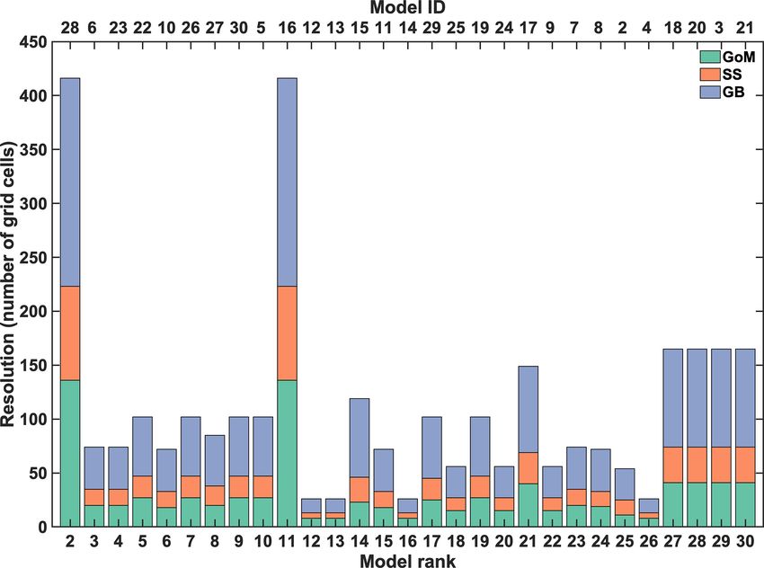
1812                    A. Laurent et al.: Evaluation of historical ESM simulations in the northwest North Atlantic Ocean

                                                                       3.3    Additional model–data comparisons for regional
                                                                              ACM

                                                                       While the resolution of the ESMs does not allow for a com-
                                                                       parison at smaller spatial scales, we further compare the re-
                                                                       gional ACM to cross-shelf transects and station observations
                                                                       (Fig. 9) along the Halifax Line (see Fig. 1). The ACM re-
                                                                       produces the seasonal variation and the vertical gradient in
                                                                       chlorophyll and nitrate along the transect (Fig. 9), although
                                                                       the simulated distributions are smoother than the glider ob-
                                                                       servations. The summer subsurface chlorophyll maximum is
                                                                       located at the appropriate depth (28 m simulated versus 32 m
                                                                       observed, on average). The ACM somewhat underestimates
                                                                       the depth of the nitracline in the offshore waters (34 m ver-
                                                                       sus 43 m, x > 150 km) and overestimates surface nitrate in
                                                                       spring and fall, as seen in Fig. 4.
                                                                          Station 2, which is located nearshore on the Halifax Line
Figure 8. Model average (gray bars) and specific (dots) ranking.       (see Fig. 1), provides additional, vertically resolved informa-
The final ranking is shown on the y axis. Hidden coinciding ranks      tion with high temporal resolution that is useful for model
(models 2, 3, 6, 10, 11, 18, 27, 28 and 30) are provided in Table 2.   validation (Fig. 10). At this location, the ACM reproduces
                                                                       the annual cycle of chlorophyll and nitrate. Surface and sub-
                                                                       surface nitrate and chlorophyll are qualitatively reproduced
CMIP5 (6, 10) and six from CMIP6 (28, 23, 22, 26, 27 and               in all seasons except during the spring bloom, which is more
30, respectively). The most consistent in terms of individ-            pronounced and reaches deeper in the observations, although
ual and overall ranking is model 28 (best ESM); the other              the magnitude and vertical distribution of chlorophyll con-
ones having a relatively large spread. On the other side of the        centration agree well with the glider observations at this time.
spectrum, models 18, 20, 3 and 21 (Groups C and D) have                   A quantitative, point-to-point comparison of the ACM
the poorest ranks because of their consistently poor scores.           with the time series and glider observations along the Hal-
Model 2 has also consistent poor ranks for all variables. De-          ifax Line (Fig. 9) and at Station 2 (Fig. 10) is provided in Ta-
spite its poor performance with respect to nitrate, model 29 is        ble 3. The comparison indicates relatively high correlations
ranked within the mid-range of the ESMs because of the bet-            between the ACM and time series of chlorophyll (0.68–0.78)
ter performance with respect to the other variables (ranks 8–          and nitrate (0.83–0.92) along the Halifax Line as well as
15); model 7 has consistently poor performance except for              glider measurements of chlorophyll (0.85–0.94) for all sea-
chlorophyll (rank 4).                                                  sons. Correlations are high as well at Station 2 for nitrate time
   Model scores and ranking were also calculated along the             series and glider measurements of chlorophyll. The largest
boundaries of the regional model (see Fig. S10). The ranking           discrepancies with observations are found with the time se-
shows that model performance on the shelf is not necessar-             ries of chlorophyll in spring. These results indicate an overall
ily indicative of the performance along the boundaries of the          good skill of the model to reproduce the seasonal, vertically
regional model (Fig. S11, Table S2). Moreover, individual              resolved observations on the Scotian Shelf.
rankings are much more variable at the boundaries, even for
the best-performing models. The eight best ESMs along the
boundaries (22, 11, 30, 28, 16, 10, 26, 6) have an average             4     Discussion
rank of 9.2–10.5. There are no significant correlations be-
tween individual rankings, including temperature and salin-            4.1    Overall model performance on the shelf
ity. Nonetheless, there is some agreement between the shelf
and the outer boundary ranking for chlorophyll (ρ = 0.80),             There are significant discrepancies with observations and a
nitrate (ρ = 0.81) and salinity (ρ = 0.81; Fig. S12 and Ta-            large variability among ESMs in the representation of surface
ble S3). Interestingly, the agreement is better with CMIP6             temperature, salinity, chlorophyll and nitrate in the NWA
models (Table S3). However, there is no agreement for tem-             shelf (Table 2, Figs. 6 and S1–S5). A warm bias and a gen-
perature. A similar pattern is found for individual bound-             eral overestimation of surface salinity in most models indi-
aries (Fig. S13). In this case, and apart from temperature, the        cate a mismatch in the location of the Gulf Stream that in-
model ranks along the northeastern boundary agree the most             fluences conditions on the shelf, in line with the previous re-
with those from the shelf.                                             sults of Loder et al. (2015) and Saba et al. (2016). Chloro-
                                                                       phyll concentration was also systematically underestimated,
                                                                       whereas surface nitrate concentration is relatively variable

Biogeosciences, 18, 1803–1822, 2021                                                       https://doi.org/10.5194/bg-18-1803-2021
A. Laurent et al.: Evaluation of historical ESM simulations in the northwest North Atlantic Ocean 1813 Figure 9. Comparison of gliders, AZMP and model seasonal climatologies of chlorophyll and nitrate along the Halifax Line. Figure 10. Comparison of vertically resolved time series of chlorophyll (a) and nitrate (b) at Station 2 from the regional model (background), the glider transects (small dots) and the bi-monthly sampling (large dots). https://doi.org/10.5194/bg-18-1803-2021 Biogeosciences, 18, 1803–1822, 2021
1814                       A. Laurent et al.: Evaluation of historical ESM simulations in the northwest North Atlantic Ocean

Table 3. Comparison statistics between ACM and AZMP and glider observations along the Halifax Line and at Station 2.

                                                        RMSD                                      Bias                         Correlation coefficient
         Season∗                              W          S        S         F         W            S         S        F        W         S         S        F
         Halifax Line
         Chlorophyll (time series)          0.25     0.37     0.39      0.36       0.08         0.22     0.28      0.13     0.68      0.78     0.71       0.75
         Chlorophyll (glider)               0.22     0.42     0.25      0.22      −0.14         0.13     0.17      0.04     0.88      0.78     0.94       0.85
         Nitrate                            2.99     2.73     2.13      1.77       0.76         2.03     0.74      1.27     0.90      0.83     0.85       0.92
         Station 2
         Chlorophyll (time series)          0.26     1.74     0.52      0.30       0.05      −0.56       0.26      0.01     0.64      0.22     0.48       0.82
         Chlorophyll (glider)               0.15     1.06     0.31      0.17      −0.03      −0.46       0.25      0.02     0.87      0.69     0.91       0.93
         Nitrate                            0.96     1.57     1.58      1.37       1.19       1.62       0.26      0.58     0.85      0.86     0.91       0.94
       ∗ Seasons are ordered sequentially and abbreviated as W (winter, December–February), S (spring, March–May), S (summer, June–August) and F (fall,
       September–November).

between models. These patterns agree with the qualitative                              the NWA shelf. Models 7, 9 and 17 had poor scores for three
assessment of Lavoie et al. (2013, 2019). The spring and fall                          variables, model 15 was also included in the outer ensemble
blooms, which are characteristic annual features of the NWA                            because of the misrepresentation of surface nitrate, whereas
region (Greenan et al., 2004, 2008), are absent in some and                            models 24–25 misrepresented temperature and salinity. Since
most models, respectively. The correlation between temper-                             nitrate scores neither correlate with chlorophyll nor tempera-
ature and chlorophyll scores (and to a lesser extent salinity)                         ture, the mismatch with nitrate observations is more likely re-
and the concomitant poor scores in chlorophyll and temper-                             lated to intrinsic biogeochemical model behavior rather than
ature/salinity (i.e., Group C in Fig. 7) indicate that errors                          to a mismatch in circulation, as suggested by Lavoie et al.
in surface chlorophyll concentration are partly driven by a                            (2019). Models with persistent positive or negative biases in
misrepresentation of the general circulation and, more gener-                          surface nitrate (4–5, 7–8, 11, 14, 19 and 29; Figs. S1–S5)
ally, of ocean physics. The improvement in chlorophyll from                            were selected because they misrepresent the seasonal nitrate
CMIP5 to CMIP6 in some models without an associated im-                                dynamics, and therefore the other biogeochemical variables
provement in temperature (see below) suggests that the errors                          driven by nitrate are questionable. Seven of the outer models
in surface chlorophyll were also driven to some extent by er-                          were different generations (CMIP5 and CMIP6) of the same
rors in the biogeochemical model component. Lavoie et al.                              model, i.e., CanESM (2, 19), CESM (3, 20–21) and NorESM
(2019) indicated that the misrepresentation of primary pro-                            (18, 29), which also had low ranks along the ACM bound-
duction in the NWA may be associated with the misrepresen-                             aries. Their large scores imply that they have fundamental
tation of particulate organic matter sinking and remineraliza-                         issues with representing biogeochemistry in the NWA.
tion in the subsurface layer. They found an annual subsurface                             The inner ensemble includes 11 models (6, 10, 12–13, 16,
nitrate peak in CanESM2, GFDL-ESM2M, NorESM1-ME                                        22–23, 26–28, 30; Table 1). Can those be used as a multi-
and CESM1-BGC (models 2, 7, 18 and 3, respectively) sim-                               model (optimal) ensemble to characterize the future state of
ilar to the high surface nitrate found in this study (Figs. S1                         the NWA shelf region? Unfortunately, we found that an en-
and S3). However, all these models had poor scores in our                              semble mean of the best CMIP5 or CMIP6 models poorly
assessment and therefore do not provide an appropriate rep-                            represents historical surface fields due to the large variability
resentation of the biogeochemistry on the NWA shelf (Fig. 8)                           within the ensemble (Fig. 5) and the biases in the ensemble
or along the ACM boundaries (Fig. S11). However, it is not                             surface temperature, salinity and chlorophyll concentration
possible, and beyond the scope of this work, for us to draw                            (Fig. 4). Model 28 (MPI-ESM1-2-HR, CMIP6) was the only
conclusions about the source of the regional mismatch in sur-                          ESM with good performance for all variables and is there-
face chlorophyll and nitrate in the ESMs.                                              fore the most appropriate to represent surface conditions in
   Following Rickard et al. (2016), who used a similar rank-                           the NWA shelf.
ing procedure, the 29 ESMs can be divided into an inner and                               The regional model clearly outperformed the ESMs in our
an outer model ensemble of the NWA shelf. The outer en-                                assessment, with a consistent representation of the surface
semble includes 18 models that clearly misrepresent surface                            and subsurface fields in all shelf areas. The high spatial res-
conditions in the NWA shelf (models 2–5, 7–9, 11, 14–15,                               olution of the regional model also allowed for a fine-scale
17–21, 24–25 and 29) and was selected as follows. The seven                            model validation that was not possible for the ESMs. The
models with lowest ranks (2–4, 8, 18, 20–21) were included                             complementary glider transects and time series stations pro-
because they consistently misrepresent all surface fields on                           vide a high-resolution dataset of in situ chlorophyll and ni-

Biogeosciences, 18, 1803–1822, 2021                                                                              https://doi.org/10.5194/bg-18-1803-2021
A. Laurent et al.: Evaluation of historical ESM simulations in the northwest North Atlantic Ocean 1815
trate concentrations and show that the regional model re-
solves seasonal and vertical variations in chlorophyll and ni-
trate on the Scotian Shelf, something that none of the ESMs
were able to reproduce.
4.2 Model performance along the regional model
boundaries
The assessment of an ESM’s performance on the NWA shelf,
as presented above, is necessary prior to using its results, for
example, to estimate historical and future trends in physical
and biogeochemical tracers (Lavoie et al., 2013, 2019) and
their effects on upper trophic levels (e.g., Bryndum-Buchholz
et al., 2020b; Stortini et al., 2015). For regional downscaling,
an ESM’s performance along the boundaries of the regional
model is critical (e.g., Lavoie et al., 2020). We found sig-
nificant differences between model performance on the shelf Figure 11. Resolution of the 29 ESMs ordered by their overall rank
and along the ACM boundaries and more variability in model (see Fig. 8).
performance for the latter. At the boundaries, all models have
at least one variable that is poorly represented (Fig. S11).
Surprisingly, there is no relationship between ESM ranking are in agreement with the 1976–2005 scores described in
on the shelf and at the ACM boundaries for temperature. Sect. 3.2 (see Fig. S14), showing the robustness of our cal-
Given the importance of large-scale circulation in the region, culations despite the heterogeneous dataset. The only sig-
some agreement was expected. The mismatch could be ex- nificant differences are with models 30 and 21, which have
plained by a lesser control of large-scale currents on shelf improved and degraded 2000–2014 scores for temperature,
temperature, although ESM biases for temperature and salin- respectively. Model 21 remains at the last rank (Table 2),
ity on the shelf indicate the influence of the Gulf Stream. The but the overall rank of model 30 (UKESM1-0-LL) could be
agreement is better for the other variables (Table S3). Among somewhat higher than indicated in Fig. 8.
the 10 best ESMs along the ACM boundaries, 8 are included
in the inner ensemble described above; the best overall ESM 4.4 Impact of spatial resolution
on the shelf (model 28) is ranked third at the boundaries.
Similarly, models with poor performance on the shelf (3, 18, In general, the coarse horizontal resolution of the ESMs af-
20–21) also had poor scores at the boundaries. The inner en- fects the representation of the NWA region in comparison
semble can therefore be used as a guide for ESM selection in to the regional model, particularly on the relatively narrow
the NWA region. Scotian Shelf. The poor representation of coastal areas is a
known limitation of global models (Holt et al., 2017) and re-
4.3 Uncertainties in score calculations sults in a global underestimation of primary productivity in
these regions (Bopp et al., 2013; Schneider et al., 2008).
We used a heterogeneous dataset to calculate error statis- There is no correlation between grid resolution and ESM
tics. Also, the regional model simulated the period 2000– rank (Fig. 11) despite the fact that the best overall ESM
2014, whereas the time range of 1976–2005 was used with (MPI-ESM1-2-HR) also has the highest resolution (Table 1).
the CMIP models, for consistency in their comparison. For This result shows that higher grid resolution, as called for
surface salinity, chlorophyll and nitrate, Lavoie et al. (2013) by Lavoie et al. (2013) for the NWA and by McKiver et al.
found negligible historical trends (1970s–2000s) in a multi- (2015) for the global ocean, is necessary but is not a guar-
model comparison. For surface temperature, they found an antee for improved model performance at this time. In fact,
increase in temperature < 0.5 ◦ C over this period, which some very-coarse-resolution models from the CMIP5 group
is very small in comparison to the inter-model differences were ranked as well as or better than the other models, and
(Figs. S1–5a–c). Also, surface temperature is overestimated models with the second-highest resolution (3, 18, 20–21) had
in the GoM, whereas the trend would result in an underesti- all low ranks. The improved ranks at constant (e.g., models
mate. Hence, the scores should not be affected by time dif- 22, 24, 25, 28) and even lower (model 29) ocean grid reso-
ferences between model and observation datasets. lution in the CMIP6 group (Table 2, Fig. 12) were also an
Since the period 2000–2014 is available for the CMIP6 indication that the discrepancies with observations, and the
models, we calculated the scores over this period to be con- improvement in the CMIP6 models (see below), were not
sistent with the regional model simulation and the chloro- associated with the ocean grid resolution but rather resulted
phyll and temperature observations. The 2000–2014 scores from the physical and biogeochemical setup of the models.
https://doi.org/10.5194/bg-18-1803-2021 Biogeosciences, 18, 1803–1822, 20211816 A. Laurent et al.: Evaluation of historical ESM simulations in the northwest North Atlantic Ocean
Another hint at the lack of relationship between resolution rank was not very different between the two CMIP groups,
and model rank is the limited improvement with the high- i.e., R = 16.8 and 14.9 for CMIP5 and CMIP6, respectively
resolution MPI model in the CMIP5 group (MPI-ESM-MR), (Fig. 8, Table 2). The change in performance between the
despite higher model grid resolution compared to its lower- two generations of models can be assessed by evaluating the
resolution counterpart (MPI-ESM-LR; Table 2). The lack of subset of models that are available for CMIP5 and CMIP6.
correlation between model resolution and performance on There are nine such models (Fig. 12). All CMIP6 models
the NWA shelf is not surprising as all ESMs are still coarse have improved overall ranks, indicating better performance
and do not explicitly resolve shelf-scale processes but rather (Fig. 12). The overall improvement was large only for mod-
rely on their parameterization. Much higher resolution will els that had average to low ranks in the CMIP5 group (ranks
be necessary to refine the projections in coastal areas (e.g., 15–22, x axis in Fig. 12). Temperature and salinity did not
Holt et al., 2017; Saba et al., 2016), which is not currently improve except for GFDL-ESM2M and NorESM2-LM (and
computationally feasible in ESMs (Holt et al., 2009, 2017). CanESM5 for salinity) and degraded in some cases. Mod-
els with poor scores for temperature and salinity (CESM2,
4.5 Impact of biogeochemical model structure GISS-E2-1-G-CC) had already poor scores in their CMIP5
version, and therefore the cause of their poor performance is
Although model performance is likely influenced by the bio- likely the same. The change in ranking is therefore mainly
geochemical model structure, we did not find a clear re- associated with better surface fields for chlorophyll and ni-
lationship between the type of biogeochemical model and trate. This is particularly the case for model pairs 3, 5, 6 and
performance. Here, we only refer to the model type be- 8, which ranked much better for chlorophyll (+8.2) and ni-
cause the same model may have different parameterizations trate (+11.0) in the CMIP6 group (Fig. 12). The chlorophyll
when used by different groups. While the inner and outer en- rank in model pair four improved significantly (+18) but this
sembles share only three biogeochemical models (PISCES, improvement was counteracted by degraded temperature and
HAMOCC, TOPAZ2) out of 13, there was no indication of nitrate ranks. The lack of general improvement in surface
consistently better performance for the biogeochemical mod- temperature indicates that the temperature bias detected in
els in the inner ensemble. For example, models using simi- the CMIP5 group was not solved in CMIP6, as seen in Fig. 4.
lar ocean biogeochemistry (e.g., PISCES: 5, 12–14 (CMIP5), We can only speculate about the source of improvement in
22 and 26 (CMIP6), and HAMOCC: 15–16, 18 (CMIP5), the CMIP6 models. For specific changes in the CMIP6 model
28–29 (CMIP6)) had very different ranks, with no obvious versions, the reader is referred to the references listed in Ta-
relationship between overall model rank and the ocean bio- ble 1. Kwiatkowski et al. (2020) recently showed that pro-
geochemical model component. Moreover, five and four bio- jected surface temperature, nitrate and net primary produc-
geochemical models were represented in the five best-ranked tion differ significantly in CMIP5 and CMIP6 model ensem-
ESMs on the NWA shelf and outer ACM boundaries, respec- bles. Higher climate sensitivity in CMIP6 models partly ex-
tively, similar to previous findings by Rickard et al. (2016). plains this difference but the source of change in primary pro-
Lavoie et al. (2019) suggested that the PISCES biogeochem- duction was not resolved. In the historical simulations, better
ical model may underestimate subsurface remineralization surface chlorophyll and nitrate fields in CNRM-ESM2-1 may
in the CNRM and IPSL models, resulting in low surface be associated with the transition from a climate model with
nutrients where the Gulf Stream detaches from the coast. ocean biogeochemistry to a fully coupled ESM, even though
Our rankings (shelf and offshore) and the spatial patterns in such transition may degrade historical simulations due to
Figs. S1–9 do not fully support this hypothesis; high surface the replacement of observations by prognostic schemes that
nitrate concentrations were present in the CNRM models are poorly constrained (Séférian et al., 2019). Updated land
throughout the region, whereas concentrations in the IPSL- and ocean biogeochemistry may have improved the repre-
CM5A models were low (except around the GoM in spring) sentation of surface chlorophyll and nitrate in MPI-ESM1-
(Figs. S1–4, S7, S9). It is unlikely that these large-scale pat- 2-HR (Müller et al., 2018), whereas the improvement in
terns are driven by upwelled Gulf Stream waters, although surface temperature and nitrate fields from GFDL-ESM2M
differences in remineralization could influence these general to GFDL-ESM4 seems to be associated with the physical
patterns. ocean component of the model, given that GFDL-ESM2G
already performed well in the CMIP5 group. Danabasoglu
4.6 Improvement from CMIP5 to CMIP6 et al. (2020) found a significant improvement for CESM2 at
the global scale but a poor representation of the Gulf Stream–
Model performance improved in the new CMIP generation North Atlantic Current system, resulting in a large surface
but not uniformly across models and variables. We note that temperature bias. This is in line with our assessment for the
two of the five best models are from the CMIP5 for both NWA shelf, where both physical and biological parameters
the shelf and the ACM boundaries rankings. Therefore, with had poor scores and the model was not found appropriate for
respect to historical conditions in the NWA region, CMIP6 shelf studies in the NWA.
models do not always have better performance. The average
Biogeosciences, 18, 1803–1822, 2021 https://doi.org/10.5194/bg-18-1803-2021You can also read