Specified dynamics scheme impacts on wave-mean flow dynamics, convection, and tracer transport in CESM2 (WACCM6) - Recent
←
→
Page content transcription
If your browser does not render page correctly, please read the page content below
Research article
Atmos. Chem. Phys., 22, 197–214, 2022
https://doi.org/10.5194/acp-22-197-2022
© Author(s) 2022. This work is distributed under
the Creative Commons Attribution 4.0 License.

        Specified dynamics scheme impacts on wave-mean flow
              dynamics, convection, and tracer transport
                        in CESM2 (WACCM6)
                      Nicholas A. Davis1 , Patrick Callaghan2 , Isla R. Simpson2 , and Simone Tilmes1
        1 Atmospheric Chemistry Observations and Modeling Laboratory, National Center for Atmospheric Research,
                                                   Boulder, CO, USA
         2 Climate and Global Dynamics Laboratory, National Center for Atmospheric Research, Boulder, CO, USA

                                  Correspondence: Nicholas A. Davis (nadavis@ucar.edu)

                                   Received: 26 February 2021 – Discussion started: 19 March 2021
                          Revised: 21 July 2021 – Accepted: 15 September 2021 – Published: 7 January 2022

       Abstract. Specified dynamics schemes are ubiquitous modeling tools for isolating the roles of dynamics and
       transport on chemical weather and climate. They typically constrain the circulation of a chemistry–climate model
       to the circulation in a reanalysis product through linear relaxation. However, recent studies suggest that these
       schemes create a divergence in chemical climate and the meridional circulation between models and do not ac-
       curately reproduce trends in the circulation. In this study we perform a systematic assessment of the specified
       dynamics scheme in the Community Earth System Model version 2, Whole Atmosphere Community Climate
       Model version 6 (CESM2 (WACCM6)), which proactively nudges the circulation toward the reference meteo-
       rology. Specified dynamics experiments are performed over a wide range of nudging timescales and reference
       meteorology frequencies, with the model’s circulation nudged to its own free-running output – a clean test of the
       specified dynamics scheme. Errors in the circulation scale robustly and inversely with meteorology frequency
       and have little dependence on the nudging timescale. However, the circulation strength and errors in tracers,
       tracer transport, and convective mass flux scale robustly and inversely with the nudging timescale. A 12 to 24 h
       nudging timescale at the highest possible reference meteorology frequency minimizes errors in tracers, clouds,
       and the circulation, even up to the practical limit of one reference meteorology update every time step. The
       residual circulation and eddy mixing integrate tracer errors and accumulate them at the end of their characteristic
       transport pathways, leading to elevated error in the upper troposphere and lower stratosphere and in the polar
       stratosphere. Even in the most ideal case, there are non-negligible errors in tracers introduced by the nudging
       scheme. Future development of more sophisticated nudging schemes may be necessary for further progress.

1   Introduction                                                    (Birner and Bönisch, 2011; Abalos et al., 2013; Garny et al.,
                                                                    2014). But for the air that ascends up through the depth of the
Anthropogenic and natural emissions of gases and aerosols           stratosphere, its fate is tied to the tug-of-war of the seasons
have substantial human and ecological consequences by               (Ploeger and Birner, 2016). Throughout the annual cycle the
virtue of atmospheric transport. In the troposphere, sporadic       residual circulation reverses course from north to south and
convection in the tropics rapidly lofts boundary layer air to       south to north, sloshing the air back and forth on a long,
high altitudes where it can slowly ascend through the trop-         multi-year journey to the poles where it finally seeps back
ical tropopause layer into the middle atmospheric Brewer–           down to the troposphere. Mixing by breaking waves recircu-
Dobson circulation (Fueglistaler et al., 2009; Butchart,            lates some of this air, increasing its stratospheric residence
2014). Some of this air is swept through the shallow branch         time beyond what would be predicted by residual circulation
of the circulation, where it quickly returns to the troposphere     trajectories alone (Garny et al., 2014). In the troposphere, air

Published by Copernicus Publications on behalf of the European Geosciences Union.
198                                                                             N. A. Davis et al.: Specified dynamics impacts

is rapidly mixed throughout the extratropics (Waugh et al.,        reproduce most of the lower-stratospheric ozone loss using
2013; Yang et al., 2019), with nearly half of the residual cir-    reanalysis meteorology, though not in the deep tropics.
culation mass transport occurring via moist diabatic ascent in        Specified dynamics schemes are a modeling technique to
the storm tracks (Pauluis et al., 2008).                           constrain known circulation variability and isolate its role
   This global transport is especially important in the con-       in driving chemical weather and climate. They are also im-
text of halogens; radiatively active aerosols like black carbon    portant tools for evaluating chemistry and physics schemes,
and sulfates; and health-relevant species including ground-        interpreting field campaign observations, and performing
level particle matter, ozone, and ozone precursors includ-         chemical forecasts. Specified dynamics schemes typically
ing carbon monoxide. Oceanic emissions of reactive chlo-           consist of a linear relaxation of fields such as temperature and
rine and bromine species mediate tropospheric ozone (Yang          horizontal winds to a reference meteorology, which is almost
et al., 2005) and can be transported up to the stratosphere        always a reanalysis product. More sophisticated techniques
where they contribute to spring ozone loss (Daniel et al.,         include NASA’s replay, in which the model is replayed af-
1999; Salawitch et al., 2005; Sinnhuber et al., 2009; Hos-         ter an initial integration with the tendencies needed to match
saini et al., 2017). Additionally, anthropogenic emissions of      the reference meteorology (Orbe et al., 2017; Wargan et al.,
CFC-11 in apparent violation of the Montreal Protocol have         2018). A chemical transport model is wholly different. While
been transported up to the stratosphere and have delayed the       it includes parameterizations of physical processes, it is de-
recovery of the ozone hole (Montzka et al., 2018; Dhomse et        void of a true dynamical core as the reference meteorology is
al., 2019).                                                        ingested directly (see, for a relevant example, Chipperfield,
   In the troposphere, carbon monoxide and particulate mat-        1999, 2006). The exchange in the aftermath of Ball et al.
ter produced by combustion contribute to premature death           (2018) indicates that one or more of these methods is defi-
and chronic health problems (Brook et al., 2010; Levy,             cient.
2015). As a tropospheric ozone precursor (Seinfeld, 1989),            Kinnison et al. (2007) showed that tracer distributions
carbon monoxide can also drive variations in global radia-         in a chemical transport model were highly sensitive to ar-
tive forcing. These constituents have a sufficiently long life-    guably minor differences in the circulation among refer-
time that they can be transported across ocean basins and im-      ence meteorologies from WACCM1b and the European Cen-
pact air quality on other continents (Jaffe et al., 1999; Pros-    tre for Medium-Range Weather Forecasts operational anal-
pero, 1999). Similarly, long-range transport of black carbon       ysis and EXP471 reanalysis. Analyses of the models in the
aerosols can have profound impacts on Arctic climate (Shin-        Chemistry-Climate Model Initiative (CCMI) indicate that the
dell et al., 2008) and may be a major driver of observed           intermodel spread in the climatological meridional circula-
tropical expansion (Allen et al., 2012; Kovilakam and Maha-        tion in specified dynamics simulations is as large or larger
jan, 2015; Zhao et al., 2020). However, transport can occur        than that in corresponding free-running simulations (Orbe et
along different pathways depending upon whether the emis-          al., 2018; Chrysanthou et al., 2019; Orbe et al., 2020). Un-
sions occur over land or ocean and can be especially sensitive     fortunately, the different models in CCMI use different spec-
to the configuration of the large-scale atmospheric circula-       ified dynamics techniques and reference meteorologies, so it
tion (Yang et al., 2019). Recent work suggests that transport      is difficult to isolate the cause of this divergence in the circu-
processes make substantial contributions to hazardous peaks        lation.
in summertime ozone (Kerr et al., 2019) and that variations           There is evidence that shorter relaxation timescales lead
in the latitude of the tropospheric jet project directly onto      to an improved simulation of temperature variability (Mer-
surface ozone (Barnes and Fiore, 2013; Kerr et al., 2020).         ryfield et al., 2013), but at the expense of damping con-
The particular nature of this transport is difficult to quantify   vective transport (Orbe et al., 2017) and reducing tropical
because it spans multiple orders of magnitude in time and          stratospheric upwelling (Hardiman et al., 2017). Some stud-
space.                                                             ies explicitly nudge the rotational part of the flow on a faster
   A recent exchange in the literature illustrates the degree      timescale than the divergent part of the flow (Löffler et al.,
to which circulation uncertainty can lead to opposing con-         2016; van Aalst et al., 2004), with the goals being to con-
clusions. Ball et al. (2018) reported that two chemistry–          strain the more certain aspect of the circulation and to allow
climate models forced by reanalysis meteorology in so-called       the convection scheme more freedom. Temperature nudging
“specified dynamics” configurations were unable to repro-          functions as diabatic heating and modulates the strength of
duce the recently observed decline in lower-stratospheric          the meridional circulation, which leads to systematic errors
ozone. If true, it would open up roles for novel chemistry         in the circulation and in tracers such as ozone (Miyazaki
or unaccounted-for emissions of ozone-depleting substances.        et al., 2005; Akiyoshi et al., 2016). More exotic nudging
Shortly thereafter, Chipperfield et al. (2018) reported that a     techniques, such as climatological anomaly (Zhang et al.,
chemical transport model was able to reproduce the ozone           2014) and zonal anomaly nudging (Davis et al., 2020), have
trends when using the same meteorology. Wargan et al.              revealed that the nudging of zonal mean temperatures can
(2018) also reported that a replay model simulation could          be a major source of error. However, it is often desirable
                                                                   to nudge temperatures to ensure that temperature-dependent

Atmos. Chem. Phys., 22, 197–214, 2022                                                 https://doi.org/10.5194/acp-22-197-2022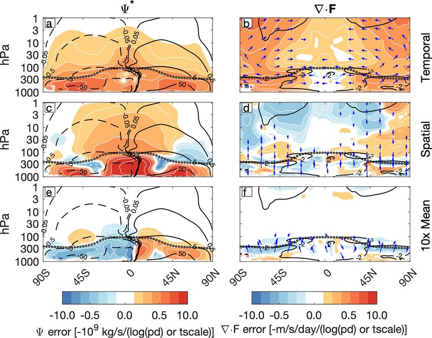
N. A. Davis et al.: Specified dynamics impacts                                                                               199

chemistry, water vapor, and microphysical processes in the         however, we use an alternative dynamical-core-independent
model are consistent with the real atmosphere (Solomon et          scheme that applies nudging as physics tendencies controlled
al., 2015, 2016; Froidevaux et al., 2019). We cannot just for-     via the “nudging” namelist (see Sect. 9.6 of the CAM6 user’s
sake temperature nudging.                                          guide). For a nudged variable, x, the nudging tendency is ap-
   In this study, we perform a clean test of a the specified dy-   plied as a linear relaxation of the form
namics scheme in CESM2 (WACCM6) in which we nudge
                                                                   ∂x        (x − xref )
the model to reference meteorology created by itself. In this           = −W             ,                                    (1)
configuration, we fully eliminate errors and uncertainty as-       ∂tsd          τ
sociated with using reference meteorology from a different         where xref is the reference meteorology value at the next ref-
modeling system but also expand the possible phase space           erence meteorology update step, τ is the relaxation timescale,
of our analysis to its practical limits. An exhaustive set of      and W is a window function that limits the spatial domain
simulations in which both the nudging timescale and mete-          over which the tendency is applied. In this formulation, the
orology frequency are varied reveals coherent, global pat-         nudging proactively pulls the model state toward the next in-
terns of circulation error that project onto errors in strato-     stantaneous reference meteorology value. The “SD” scheme
spheric and tropospheric ozone and carbon monoxide. These          instead calculates xref as a linear interpolation between the
tracers have contrasting source and loss regions. Ozone is         two nearest reference meteorology values, which attempts to
photochemically produced in the tropical stratosphere, while       correct the future state based on present disagreement.
carbon monoxide is produced at the surface by combustion              W is set to 1 below 1 hPa and linearly tapers to 0 between 1
and photochemically produced in the mesosphere and lower           and 0.1 hPa to avoid numerical instabilities related to nudg-
thermosphere. Together they may provide a comprehensive            ing in the presence of atmospheric tides and large gravity
sample of circulation impacts on tracer transport. While we        wave tendencies. In the simulations in this study we nudge
highlight one particular configuration that minimizes errors       the full zonal wind, meridional wind, and temperature, al-
in the circulation, clouds, and tracers, substantial room for      though the model can be configured to nudge any combina-
improvement remains and will likely require innovating be-         tion of these variables, as well as water vapor.
yond linear relaxation of the full meteorology.                       In computing the tendencies there are three relevant step-
                                                                   ping intervals: Nstep = 48, the number of dynamical time
                                                                   steps per day; Nobs , the number of times per day that ref-
2   Model configuration                                            erence meteorology is available; and Nupdate , the number of
                                                                   times per day the nudging tendency in Eq. (1) is updated. We
The CESM2 (WACCM6) finite-volume dynamical core (Get-              set Nupdate to 48 so that the nudging tendency is updated ev-
telman et al., 2019) is run at 1◦ horizontal resolution with       ery dynamics time step with the most recent value of x from
110 vertical levels from the surface to approximately 140 km       the specified dynamics simulation. Reanalysis output is typi-
in the lower thermosphere for 1 year from 1 January to             cally provided every 6 h (Nobs = 4) or 3 h (Nobs = 8). Here, a
31 December 2018. We run so-called “F” compset cases,              free running simulation is used to generate the reference me-
with prescribed sea surface temperatures and sea ice and pre-      teorology every 30 min dynamics time step. For cases other
scribed vegetation phenology based on satellite observations.      than Nobs = 48, we subsample the instantaneous output at
Solar forcings, greenhouse gas lower boundary conditions,          equally spaced intervals. While there is some evidence that
volcanic emissions, and other surface emissions are pre-           the use of averaged fields may produce more realistic strato-
scribed according to the CMIP6 SSP5-8.5 scenario (O’Neill          spheric transport (Orbe et al., 2017), it is not clear whether
et al., 2016). Anthropogenic emissions of volatile organic,        this would apply to the very-high-frequency meteorology ex-
non-methane volatile organic, and other compounds are pre-         amined here.
scribed by the Copernicus Atmosphere Modeling Service 81              A suite of specified dynamics simulations are then used
dataset (Granier et al., 2019), while fire emissions are pre-      to explore how variations in the nudging parameters Nobs ,
scribed by the Fire INventory from NCAR version 1 dataset          the reference meteorology frequency, and τ , the nudging
(Wiedinmyer et al., 2011). The quasi-biennial oscillation is       timescale, shape the errors in the resulting simulation. This
not prescribed but is instead spontaneously driven by inter-       is advantageous because our analysis will not be obscured by
nally generated waves (Garcia and Richter, 2019). All simu-        differences in topography, physics, and dynamical cores if
lations have identical initial conditions derived from the same    we were to nudge our model to reanalysis output. It will also
spin-up run on 1 January 2018.                                     allow us to explore the parameter Nobs over a larger range of
   There are two specified dynamics implementations in             values up to the limit of a new reference meteorology value
CESM2. “SD” compsets are configured to apply nudging               every time step.
only within the finite-volume dynamical core as described             To validate the specified dynamics scheme, a null test with
in Kunz et al. (2011), with the applied tendencies controlled      a 30 min nudging timescale in which the reference meteorol-
via the “met” namelist (see Sect. 6.4 of the CAM6 user’s           ogy is sampled at every 30 min model time step (Nobs = 48)
guide, URL in the Code and data availability section). Here,       and the tendencies are updated every time step (Nupdate = 48)

https://doi.org/10.5194/acp-22-197-2022                                              Atmos. Chem. Phys., 22, 197–214, 2022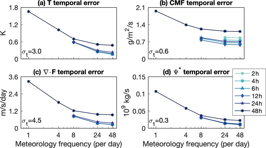
200                                                                            N. A. Davis et al.: Specified dynamics impacts

must return nudging tendencies that remain zero and model
states that perfectly match the evolution of the reference me-
teorology. The scheme fails this null test in the current im-
plementation of CESM2 because, while the reference mete-
orology is generated at the end of the dynamics step and be-
fore the physics step, the nudging tendencies are applied at
the end of the physics step when all other parameterizations
have already modified the model state. If the physics order
is modified so that the nudging tendencies are calculated and
applied at the start of the physics step, the model passes this
null test. Future versions of CESM2 will contain this correc-
tion to the physics order.
   We test six different nudging timescales: 2 h, a very short
timescale to constrain high-frequency variability; 4 and 6 h,
short timescales to constrain sub-diurnal variability; 12 and
                                                                  Figure 1. The stability of specified dynamics configurations over
24 h, moderate timescales to constrain diurnal variability;
                                                                  the full meteorology frequency/nudging timescale ranges examined
and 48 h, a longer timescale to constrain synoptic variability.   here. “Stability” refers to whether the configuration requires an in-
We also test five different meteorology frequencies: 1 update     crease in the finite-volume advection subcycling. See text for de-
per day, the arbitrary limit of the nudging scheme; 4 updates     tails.
per day, equivalent to 6-hourly reanalysis meteorology; 8 up-
dates per day, equivalent to 3-hourly reanalysis meteorology;
24 updates per day; and 48 updates per day, the practical limit   the root-mean-square spatial error (RMSSE), and the sign-
of an update every time step. Combinations of nudging pa-         adaptive mean error (SAME). The root-mean-square tempo-
rameters that require an increase in the “nsplit” parameter,      ral error of a variable x is defined as
the finite-volume advection subcycling, to run without errors                          q
are considered here to be unstable. The 2 and 4 h nudging         RMSTE(p, φ, λ) = (xs.d. (t, p, φ, λ) − xref (t, p, φ, λ))2 , (2)
at 1, 4, and 8 updates per day and 6, 12, and 24 h nudging
                                                                  where t, p, φ, and λ are the time, pressure, latitude, and lon-
at 1 and 4 updates per day require an increase in advection
                                                                  gitude coordinates; the overbar indicates the time mean; xs.d.
subcycling, so they are not considered viable configurations.
                                                                  is the value of x in the specified dynamics simulation; and
They are generally cases in which the nudging timescale is
                                                                  xref is the value of x in the reference simulation. In some
close to or faster than the meteorology frequency. All other
                                                                  cases we vertically and meridionally average this error. The
combinations are stable, resulting in 18 distinct specified dy-
                                                                  vertical and meridional average of some variable x between
namics simulations. See Fig. 1 for a summary of all of these
                                                                  two pressure levels p1 and p2 , with p1 > p2 , is given as
configurations and their stability.
   For temperature, convective mass flux, and ozone and car-                          Zp1           Z90
bon monoxide mole fraction, we archive the output at every                  1                  π
                                                                  hxi =                                     [x] cos(φ)dφ dp,       (3)
model time step to ensure that our error analysis captures              (p1 − p2 )            360
                                                                                     p=p2           φ=−90
the full variability in each field. For wave-mean flow dynam-
ics and transport we archive daily average fields, including      where brackets indicate the zonal mean. Errors are averaged
daily average eddy fluxes of heat, momentum, and tracers.         from the tropopause pressure to 1000 hPa for a tropospheric
All eddy fluxes are calculated online in the model every time     average, averaged from 1 hPa to the tropopause pressure for
step, such that their daily average is the true average. See      a stratospheric average (approximating the stratopause as
the Code and data availability section for information on the     1 hPa), and averaged from 1 hPa to 1000 hPa for a global av-
modifications to the source code necessary for this output.       erage. The root-mean-square spatial error is defined as
   While the El Niño–Southern Oscillation was generally                         s
neutral in 2018, the reference simulation generated a sudden                                                          2
warming on 21 February, which was remarkably close to the         RMSSE(t) =        [xs.d. (t, p, φ)] − [xref (t, p, φ)]     . (4)
observed sudden warming on 18 February and may impact
the results for the Northern Hemisphere.                          The root-mean-square temporal error, which we will refer to
                                                                  hereafter as “temporal error”, quantifies the average error in
                                                                  temporal variability, while the root-mean-square spatial er-
3   Methods                                                       ror, which we will refer to hereafter as “spatial error”, quan-
                                                                  tifies the error in the zonal mean structure at each time step.
Model performance is assessed using three measures of dis-            To quantify the mean bias for fields that are not single-
agreement: the root-mean-square temporal error (RMSTE),           signed, we modify the formula for the mean bias to account

Atmos. Chem. Phys., 22, 197–214, 2022                                                 https://doi.org/10.5194/acp-22-197-2022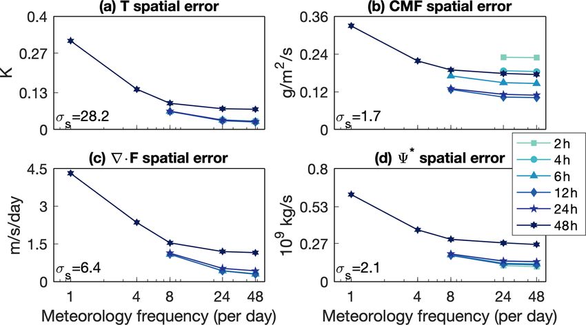
N. A. Davis et al.: Specified dynamics impacts                                                                                201

for the average sign of the field in the reference meteorology       The angular momentum per unit mass is
to derive the sign-adaptive mean error (SAME),
                                                                  M = a cos(φ) u + a cos(φ) ,                               (8)
SAME(p, φ, λ) = x s.d. (p, φ, λ) − x ref (p, φ, λ)
                                                                    where  = 7.292 × 10⁻⁵ per second is the rotation rate of
                 x ref (p, φ, λ)                                    Earth.
                                  .                          (5)      The EP flux is
                |x ref (p, φ, λ)|
                                                                                           ∂[M] [v 0 θ 0 ]

Positive values of the SAME greater in magnitude than the                 φ z                                  0 0
                                                                    F = F , F = ρ0                         − [M v ] ,
reference climatology indicate the field is greater in magni-                               ∂z ∂θ/∂z
tude and of the same sign. Negative values of the SAME in-
                                                                                       1 ∂[M] [v 0 θ 0 ]

                                                                                                               0 0
dicate cases where the field is weaker in magnitude but of                       ρ0                        − [M w ] ,     (9)
                                                                                       a ∂φ ∂[θ ]/∂z
the same sign as the reference climatology and cases where
the field is greater in magnitude than and of the opposite sign     where v and w are the meridional and vertical velocities, θ is
to the reference climatology. We will periodically display the      the potential temperature, and primes denote deviations from
actual mean bias and refer to both as “mean errors” but will        the zonal mean. The EP flux is parallel to the group veloc-
always use the SAME to calculate global average mean er-            ity of steady, linear Rossby waves and traces Rossby wave
rors.                                                               propagation in the meridional plane (Edmon et al., 1980). By
   In principle, the spatial and temporal error can be corrected    virtue of their intrinsic easterly phase speeds, Rossby waves
for the mean bias (see, for example, Murphy and Epstein,            gather easterly momentum from their source regions and de-
1989). However, this would require a reasonable estimate of         posit easterly momentum where they dissipate, respectively,
the long-term climatology of this particular model configu-         leading to acceleration of and drag on westerly flow.
ration, for which we only have a single year. While our dis-           The TEM residual streamfunction is given by
cussion will address the spatial, temporal, and mean error as
separate terms, it should be noted that they are not orthogo-                             Zz
                                                                      ∗
nal. In all cases we examine the time mean of all errors and        9 = −2π a cos(φ)           [v ∗ ]ρ0 dz,                   (10)
fields over the entire 1-year simulation period.                                          ∞

3.1   Transformed Eulerian mean dynamics                            where [v ∗ ] is the TEM residual circulation meridional veloc-
                                                                    ity,
We will use the transformed Eulerian mean (TEM) frame-
                                                                                    ∂ [v 0 θ 0 ]

work to more directly delineate the relationships between              ∗
                                                                    [v ] = [v] −                   .                          (11)
errors in eddy-mean flow dynamics and chemical transport.                          ∂z ∂θ/∂z
The TEM zonal mean zonal momentum equation in log-
pressure coordinates is given by                                    As it is equivalent to the Eulerian mean flow in the absence
                                                                    of meridional eddy heat fluxes, the TEM residual circulation
∂[u]          1                     1
     =              [∇] · F −                  ∇                    can be interpreted as that part of the meridional flow with the
 ∂t     ρ0 a cos(φ)           2π a ρ0 cos2 (φ)
                                  2
                                                                    adiabatic recirculations driven by the meridional eddy heat
     · (R90 ∇9 ∗ )[M] + [X],

                                                             (6)    flux removed. This can also be deduced from the equiva-
                                                                    lence between the TEM meridional circulation and the Eu-
where u is the zonal wind, F is the Eliassen–Palm (EP)              lerian mean meridional circulation in isentropic coordinates
flux vector, R90 = {0, −1; 1, 0} is the 90◦ rotation matrix, 9 ∗    (Juckes, 2001). It is therefore a quasi-Lagrangian approxima-
is the TEM residual streamfunction, M is the angular mo-            tion of zonal mean parcel trajectories, which gives it greater
mentum per unit mass, X is a catch-all for non-conservative         utility for examining transport than the Eulerian mean.
forces including friction, a is the radius of the Earth, and ∇ is
the zonal mean divergence operator in spherical coordinates
                                                                    3.2   Chemical transport
given as

           1     ∂            ∂
                                                                   Chemical transport is assessed with the TEM transport equa-
∇=                  cos(φ),        .                          (7)   tion,
       a cos(φ) ∂φ           ∂z
The log-pressure height z is given by the transformation            ∂[χ ]  1             1
                                                                          = ∇ ·Fχ −               (R90 ∇9 ∗ )
z = −H ln(p/pr ), where p is the pressure, pr = 1000 hPa             ∂t    ρ0       2π aρ0 cos(φ)
is the reference surface pressure, and the scale height H                 · ∇[χ] + [S],                                       (12)
is taken as 6800 m. Log-pressure density ρ0 is given by
ρ0 = ρr (p/pr ) = p/(Hg), where g is the acceleration due to        where χ is the mole fraction of some chemical species, S
gravity.                                                            is its source/sink, and F χ is the TEM eddy transport vector

https://doi.org/10.5194/acp-22-197-2022                                               Atmos. Chem. Phys., 22, 197–214, 2022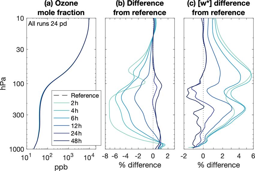
202                                                                                 N. A. Davis et al.: Specified dynamics impacts

given by

                            ∂[χ] [v 0 θ 0 ]

       φ z                                     0 0
F χ = Fχ , Fχ = ρ0                          − [v χ ] ,
                             ∂z ∂[θ]/∂z
        1 ∂[χ ] [v 0 θ 0 ]

   ρ0                      + [w0 χ 0 ] .                       (13)
        a ∂φ ∂[θ]/∂z

It is not coincidental that this has the same form as the EP
flux vector, as the EP flux is simply the TEM eddy transport
vector for angular momentum. The characteristic feature of
the TEM is that for all tracers, the adiabatic transport by the
mean flow induced by the meridional eddy heat fluxes is ab-
sorbed into the eddy transport itself.                                 Figure 2. Globally and vertically averaged root-mean-square tem-
                                                                       poral error in (a) temperature, (b) convective mass flux, (c) EP flux
                                                                       divergence, and (d) the TEM streamfunction as a function of me-
4   Global errors in meteorology
                                                                       teorology frequency (horizontal axis) and nudging timescale (see
                                                                       legend). For reference, the globally and vertically averaged tempo-
Temporal (Fig. 2) and spatial (Fig. 3) errors in temperature,          ral standard deviation of each field is shown in each panel.
the EP flux divergence, and the TEM streamfunction de-
crease exponentially with increasing meteorology frequency
and decrease slightly with decreasing nudging timescale. Re-
call that the nudging timescale refers to the linear relaxation
timescale in Eq. (1), while meteorology frequency refers to
the number of times per day that the reference meteorology is
updated in the specified dynamics scheme. The errors asymp-
tote toward the maximum possible meteorology frequency of
48 per day – exposing a lower limit of 10 % temporal error
and 0.1 %–10 % spatial error relative to the temporal and spa-
tial variability1 . Mean errors do not scale with meteorology
frequency at all and instead decrease with increasing nudg-
ing timescale (Fig. 4; if one neglects the combination of 48 h
and 1 per day simulation, which is a major outlier for the
circulation metrics). For temperature and convective mass              Figure 3. As in Fig. 2 but for the root-mean-square spatial error,
flux, both thermodynamic quantities, the mean error disap-             and the globally and vertically averaged spatial standard deviation
                                                                       of each field is shown in each panel.
pears at longer nudging timescales (Fig. 4a, b), though for
the circulation the mean errors reach a minimum at a 24 h
timescale (Fig. 4c, d). At a longer nudging timescale of 48 h,         itself. It is indeed the case that the global convective mass
the nudging is too gentle to have a material impact on the             flux erroneously weakens with decreasing nudging timescale
modeled climate. Temperature, the EP flux divergence, and              (Fig. 4b), which in the tropics manifests as a robust de-
the TEM streamfunction are biased high/strong by increas-              crease below 500 hPa (Fig. 5a, b). Orbe et al. (2017) simi-
ing the nudging timescale, while the convective mass flux is           larly show that a CESM1(WACCM4) simulation nudged to
biased weak. See Figs. S1–S3 in the Supplement for errors in           Modern-Era Retrospective analysis for Research and Appli-
the zonal and meridional winds, which behave identically to            cations (MERRA) at a 5 h nudging timescale has a weak-
the errors in temperature.                                             ened convective mass flux relative to a simulation nudged to
   Temporal and spatial errors in the convective mass flux de-         MERRA at a 50 h nudging timescale. There are time-average
crease exponentially with increasing meteorology frequency             positive temperature nudging tendencies at the characteristic
but reach a minimum at a 12 h nudging timescale (Figs. 2b              altitudes of shallow and deep convective heating that may be
and 3b). At shorter and longer nudging timescales the error            acting to suppress convection (Fig. 5c). Aloft, negative tem-
increases. For parameterized processes such as clouds, nudg-           perature nudging tendencies, which may be acting in lieu of
ing presents a conundrum. Cloud heating will be built in to            cloud-top radiative cooling, scale with decreasing nudging
the reference meteorology temperature, so that nudging to              timescale and are associated with increased convective mass
the reference meteorology temperature will effectively per-            flux. Nudging, especially at a timescale shorter than 24 h, in-
form some fraction of the convective heating via the nudging           curs substantial and apparently unavoidable (Fig. 4b) penal-
   1 This is the ratio between the error and the corresponding stan-   ties in convective mass flux.
dard deviation.

Atmos. Chem. Phys., 22, 197–214, 2022                                                      https://doi.org/10.5194/acp-22-197-2022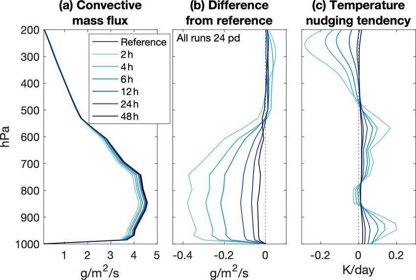
N. A. Davis et al.: Specified dynamics impacts                                                                                       203

Figure 4. As in Fig. 2 but for the mean error, and the globally and
vertically averaged absolute value of each field is shown in each
panel.

                                                                      Figure 6. Tropical stratospheric upwelling (a) mean and (b) differ-
                                                                      ence from the reference meteorology for all nudging timescales at
                                                                      24 meteorology updates per day. Tropical stratospheric upwelling
                                                                      is defined as the area average of all annual mean upwelling vertical
                                                                      velocities at each vertical level.

                                                                      2 h nudging timescale and no detectable difference at a 24 h
                                                                      nudging timescale (Fig. 6).

                                                                      5   Global errors in tracers

                                                                      Errors in ozone and carbon monoxide mole fraction in the
                                                                      troposphere and stratosphere behave similarly to errors in the
                                                                      convective mass flux (Figs. 7 and 8), with a minimum in spa-
Figure 5. Tropical convective mass flux (a) mean and (b) differ-      tial and temporal errors at 12 to 24 h nudging timescales.
ence from the reference meteorology, and (c) temperature nudging      While temporal errors are high at only the shortest and
tendency for all nudging timescales at 24 meteorology updates per     longest nudging timescales, spatial errors are especially high
day. Average taken from 20◦ S to 20◦ N.                               at nudging timescales shorter than 12 h. The temporal errors
                                                                      asymptote at around 10 %–25 % of the total variability, while
                                                                      spatial errors asymptote at a mere 0.1 %–5 %. This is proba-
   On the other hand, nudging at too long or short a timescale        bly due to the first-order influence of photochemistry on the
leads to clouds occurring at different times (Fig. 2b) and            global distribution of these tracers. Spatial error is a relatively
in different places (Fig. 3b) than the reference meteorology,         strong function of timescale, while temporal error tends to
even though it may result in minimal global mean error at             scale more consistently with meteorology frequency.
the longest nudging timescale (Fig. 4b). While spatial and               The mean errors in tropospheric and stratospheric carbon
mean errors in the convective mass flux asymptote at approx-          monoxide and stratospheric ozone mole fraction decrease
imately 10 % of the total variability, temporal errors asymp-         with increasing nudging timescale (Fig. 9a, b, d) and all but
tote at values equal to and larger than the variability.              disappear at a 48 h nudging timescale. In both regions, car-
   The positive mean error of the EP flux divergence, in-             bon monoxide is biased low. Stratospheric ozone displays a
dicating greater wave generation and wave drag, is consis-            unique dependence on meteorology frequency, although it is
tent with the positive mean error in the TEM streamfunc-              still also governed by the nudging timescale (Fig. 9c). As
tion (Fig. 4c, d). The tropical stratospheric upwelling veloc-        for the spatial and temporal errors, the mean error in strato-
ity is an especially important measure of the residual cir-           spheric ozone also reaches a minimum at the 12–24 h nudg-
culation, as it diagnoses the net transport through the trop-         ing timescale. However, the mean errors are generally small,
ical tropopause layer and into the stratosphere. Tropical up-         ranging from 5 % for stratospheric carbon monoxide to 0.1 %
welling in the lower stratosphere increases with decreasing           for stratospheric ozone.
nudging timescale, with a peak increase of 3 %–5 % at a

https://doi.org/10.5194/acp-22-197-2022                                                   Atmos. Chem. Phys., 22, 197–214, 2022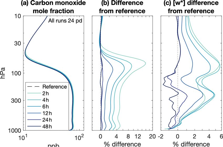
204                                                                                N. A. Davis et al.: Specified dynamics impacts

Figure 7. Globally and vertically averaged root-mean-square tem-      Figure 9. As in Fig. 7 but for the mean error, and the globally and
poral error in tropospheric (a) ozone and (b) carbon monoxide and     vertically averaged absolute value of each field is shown in each
stratospheric (c) ozone and (d) carbon monoxide. For reference,       panel.
the globally and vertically averaged temporal standard deviation of
each field is shown in each panel.

                                                                      Figure 10. Tropical ozone (a) mean and (b) percent difference from
Figure 8. As in Fig. 7 but for the root-mean-square spatial error,    the reference meteorology, and (c) residual vertical velocity for all
and the globally and vertically averaged spatial standard deviation   nudging timescales at 24 meteorology updates per day. Average
of each field is shown in each panel.                                 taken from 20◦ S to 20◦ N.

                                                                      free troposphere, which propagate up though the tropical
   These mean errors in the troposphere are surprising given
                                                                      pipe (Figs. 10c and 11c). It is unclear why the broader but
the errors in the convective mass transport. Deep convec-
                                                                      slower ascent by the residual circulation would exert a more
tion rapidly transports boundary layer air to the upper tro-
                                                                      dominant control than localized but more intense convective
posphere. This air is relatively low in ozone and relatively
                                                                      mass transport. It may be that changes in convective trans-
rich in carbon monoxide, such that convection acts to reduce
                                                                      port are more readily damped by horizontal advection than
upper tropospheric ozone (Folkins et al., 2002; Doherty et
                                                                      changes in zonal mean ascent.
al., 2005; Voulgarakis et al., 2009; Paulik and Birner, 2012)
                                                                         The serious impact of the nudging timescale and meteo-
and increase upper tropospheric carbon monoxide (Kar et al.,
                                                                      rology frequency on ozone and carbon monoxide warrants
2004; Park et al., 2009). The weakening convective mass flux
                                                                      further investigation. Errors in the tropics are consistent with
with decreasing nudging timescale (Fig. 5) should lead to ele-
                                                                      circulation differences rather than convective transport dif-
vated free-tropospheric ozone and reduced free-tropospheric
                                                                      ferences, so it seems reasonable to posit that differences in
carbon monoxide in the tropics. However, the opposite oc-
                                                                      the resolved circulation are the dominant source of the error.
curs, with reduced ozone and increased carbon monoxide
throughout the whole troposphere and the lower stratosphere
(Figs. 10 and 11). An alternative explanation is that the ac-
celeration of the residual circulation with decreasing nudging
timescale leads to anomalously negative ozone and anoma-
lously positive carbon monoxide advection tendencies in the

Atmos. Chem. Phys., 22, 197–214, 2022                                                     https://doi.org/10.5194/acp-22-197-2022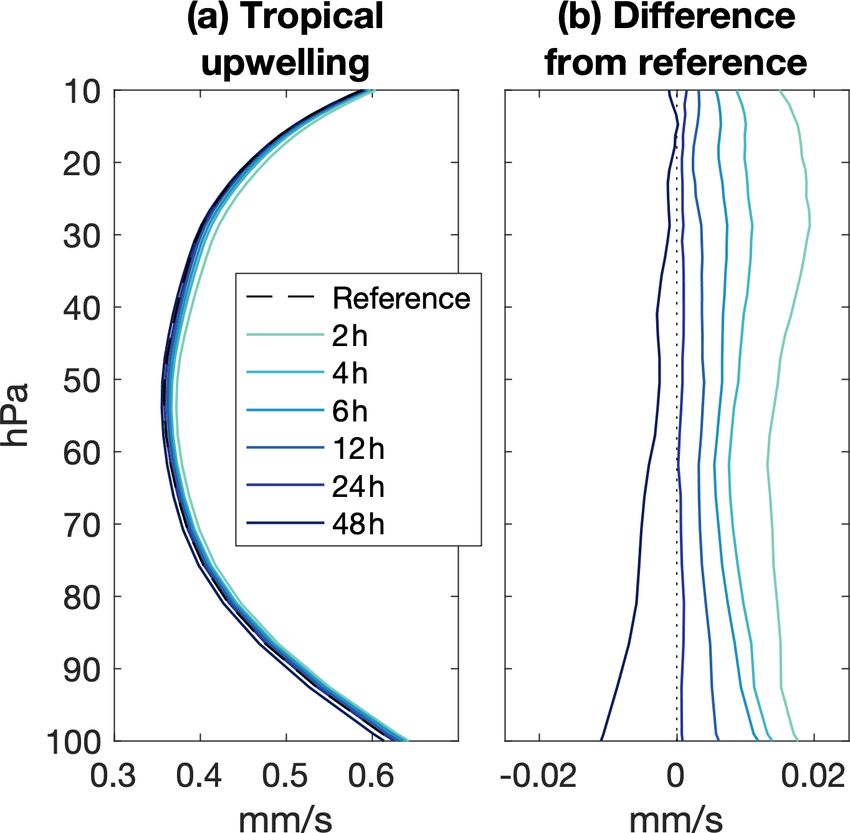
N. A. Davis et al.: Specified dynamics impacts                                                                                    205

Figure 11. As in Fig. 10 but for carbon monoxide.

                                                                 Figure 12. Negative of the projection of (a, b) root-mean-square
                                                                 temporal error, (c, d) root-mean-square spatial error, and (e, f) mean
6   Errors in eddy-mean flow dynamics
                                                                 error in the (a, c, e) TEM streamfunction and (b, d, f) EP flux and
                                                                 divergence onto the (a, b, c, d) logarithm of meteorology frequency
The systematic variation of temporal, spatial, and mean er-
                                                                 and (e, f) nudging timescale. Projection in shading (logarithmic
rors with the nudging timescale and meteorology frequency        scale), climatology in contours, and EP flux in vectors, scaled as
means that they can be reliably described by appropriate re-     in Edmon et al. (1980). In panels (a), (c), and (e) the climatologi-
gressions across the parameter space. While temporal and         cal TEM streamfunction is contoured 0.05, 0.5, 5, and 50 × 109 kg
spatial errors in the circulation appear to be governed pri-     per second, with positive values solid and negative values dashed.
marily by meteorology frequency (Figs. 2 and 3), tempo-          In panels (b), (d), and (f) the climatological EP flux divergence is
ral and spatial errors in ozone and carbon monoxide ap-          contoured every 2 m per second per day, with negative values solid.
pear to be governed by meteorology frequency and the nudg-       The tropopause is shown by the black and white dotted contour.
ing timescale, respectively (Figs. 7 and 8). Mean errors in
all fields are primarily governed by the nudging timescale
(Figs. 4 and 9). Therefore, we will focus on the regression      tern in the physical field associated with either meteorology
of temporal and spatial errors in the EP flux and its di-        frequency or nudging timescale. It is useful only as a visu-
vergence and the TEM streamfunction on meteorology fre-          alization of the structures that produce spatial error and vary
quency, while we will focus on the regression of temporal        with nudging parameters and not indicative of the change in
and spatial errors in ozone and carbon monoxide on mete-         the spatial error itself, which only has the dimension of time.
orology frequency and the nudging timescale, respectively.          As meteorology frequency decreases, the temporal error
For all fields, we will focus on the regression of mean error    in the TEM residual streamfunction increases in general pro-
on the nudging timescale. We will display the negative of all    portion to the climatology (Fig. 12a). In the troposphere, tem-
error regressions – that is, for decreasing nudging timescale    poral errors in the midlatitude Ferrel circulation, but not the
and decreasing meteorology frequency.                            Hadley cell, increase with decreasing meteorology frequency
   To examine the structure of temporal and mean errors, we      (Fig. 12a). The projection of TEM streamfunction spatial
simply project the zonal mean root-mean-square temporal er-      error is characterized by a single pole-to-pole, surface-to-
ror or mean error in each simulation onto either the loga-       stratopause cell (Fig. 12c), which suggests that the errors
rithm of meteorology frequency or onto a 1 standard devia-       arise when the solstitial residual circulation is generally too
tion change in the nudging timescale (about 15 h). For ex-       strong and expansive in one hemisphere and too weak and
amining spatial errors, we first project each field onto the     contracted in the other. In the troposphere, spatial error is
time series of its spatial error to obtain a zonal mean map      especially concentrated in the tropics and the storm tracks
and then project the maps from each simulation onto either       where there is moist diabatic ascent.
the logarithm of meteorology frequency or onto the nudg-            As meteorology frequency decreases, the temporal errors
ing timescale. One can interpret the first regression as the     in the stratospheric EP flux divergence increase poleward of
change in temporal or mean error per change in either me-        the climatological divergence and deep within the polar vor-
teorology frequency or nudging timescale. The second re-         tices, associated with errors in the meridional propagation
gression is more nuanced, as it is not the spatial error that    of Rossby waves (Fig. 12b). In the upper stratosphere the
is regressed but instead the pattern in the physical field as-   meridional position of the peak EP flux divergence domi-
sociated with variations in spatial error. The second regres-    nates the spatial error in the Northern Hemisphere, while it
sion should therefore be interpreted as the (erroneous) pat-     is instead dominated by the total magnitude of the EP flux

https://doi.org/10.5194/acp-22-197-2022                                              Atmos. Chem. Phys., 22, 197–214, 2022
206 N. A. Davis et al.: Specified dynamics impacts
divergence in the Southern Hemisphere (Fig. 12d). In both
hemispheres, this error is governed by a vertical redistribu-
tion of wave activity rather than by changes in meridional
propagation. In the troposphere, temporal errors in the EP
flux divergence increase with decreasing meteorology fre-
quency in the extratropics in proportion to the climatology.
There is no planetary-scale structure to the spatial error in
the troposphere, although it appears roughly antisymmetric
about the Equator (Fig. 12d). As in the stratosphere, this er-
ror is governed primarily by a vertical redistribution of wave
activity.
In the troposphere the TEM streamfunction and EP flux
divergence/convergence are invigorated by decreasing the
nudging timescale (Fig. 12e, f). The invigoration of the Figure 13. Percent of the temporal, spatial, and mean error in the
stratospheric TEM streamfunction is limited to the shallow (a) TEM streamfunction and (b) EP flux divergence attributable to
branch of the circulation, with the error rapidly tapering off the zonal mean or eddy fields. Whiskers indicate the maximum and
above 50 hPa. Global average mean errors in the circulation minimum across all nudging simulations.
(Fig. 4c, d) are therefore reflective of the mean error almost
everywhere in the troposphere but virtually nowhere in the
stratosphere. Here we sum the eddy and residual circulation fluxes and
The physical coupling between the wave-driven TEM convergences on the right hand side of Eq. (11) and perform
streamfunction and EP flux divergence raises the question of the same regressions as before. However, to more directly
which aspect of the circulation – the zonal mean or the eddies assess the impact of each type of transport error on ozone
– is the source of their errors (Figs. 2c, d; 3c, d). A simple di- and carbon monoxide, we multiply the error in the combined
agnostic is to “swap” either the zonal mean or eddy fields TEM residual flux and TEM eddy flux convergence by the e-
from the reference meteorology into the calculation of the folding timescale of the corresponding tracer. The timescales
TEM streamfunction and EP flux divergence in the nudged are estimated by determining the lag at which each tracer’s
simulations and recalculate the errors. The reduction in er- autocorrelation drops to 1/e in the reference run. The e-
ror between the swapped and non-swapped simulations mea- folding timescale for ozone ranges from 5 d in the tropical
sures the impact of the swapped field on the error. It is only upper troposphere and lower stratosphere to 70 d in the ex-
diagnostic and does not entertain any feedbacks between the tratropical stratosphere, while for carbon monoxide it ranges
eddies and the mean flow. from 30 d in the tropical upper troposphere and lower strato-
Temporal, spatial, and mean errors in the TEM stream- sphere to 70 d in the extratropical stratosphere (see Fig. S4).
function are overwhelmingly due to the Eulerian-mean part Both of these timescales have substantial vertical and hori-
of the circulation, while the errors in the EP flux divergence zontal structure.
are entirely due to the eddy fields (Fig. 13). The eddy fluxes With decreasing meteorology frequency, temporal errors
that comprise the EP flux divergence are merely scaled by in ozone and carbon monoxide peak at greater than 1 % and
their projection onto angular momentum and static stabil- 10 % of the climatology, respectively, in the upper tropo-
ity, so it is not so surprising that the Eulerian mean contri- sphere and lower stratosphere and in the polar stratosphere
bution is negligible. It does seem surprising that the Eule- (Figs. 14a and 15a). This pattern is mirrored by an increase in
rian mean dominates the errors in the TEM streamfunction temporal errors in the ozone and carbon monoxide flux con-
though. While the correction for the eddy recirculations is vergences with decreasing meteorology frequency (Figs. 14b
not a dominant component of the TEM streamfunction ex- and 15b). As these errors reflect the temporal error in the EP
cept in the extratropics, the errors they introduce are appar- flux divergence (Fig. 12b), they appear consistent with local
ently vanishingly small. This result instead points to tem- errors in eddy mixing.
perature nudging (Fig. 5c) directly invigorating the Eulerian However, there is a strong signal in the temporal error in
mean part of the circulation (Fig. 6, and see also Miyazaki et the ozone and carbon monoxide fluxes, but not convergences,
al., 2005; Akiyoshi et al., 2016). in the tropical upper stratosphere. This implicates the deep
branch of the residual circulation, which acts non-locally to
accumulate errors in tracers along the Equator-to-pole trans-
7 Errors in ozone and carbon monoxide and their port pathway, both up and down the tracer gradient.
transports Ozone and carbon monoxide spatial errors associated with
nudging timescale peak at up to 0.5 % in the upper tropo-
These errors in the dynamics project strongly onto ozone sphere and lower stratosphere (Figs. 14c and 15c). In the
(Figs. 14 and 15) and carbon monoxide (Figs. 16 and 17). upper troposphere and lower stratosphere, this hemispher-
Atmos. Chem. Phys., 22, 197–214, 2022 https://doi.org/10.5194/acp-22-197-2022N. A. Davis et al.: Specified dynamics impacts 207
.
Figure 16. Global average (a) root-mean-square temporal error,
(b) root-mean-square spatial error, and (c) sign-adaptive mean error
in ozone attributable to the TEM residual circulation and TEM eddy
flux convergences, based on the projections in the right column of
Figure 14. Negative of the projection of (a, b) root-mean-square Fig. 14
temporal error, (middle row) root-mean-square spatial error, and (e,
f) mean error in (a, c, e, shading) the ozone mole fraction and (b, d,
f, vectors) the combined TEM residual circulation and eddy ozone
flux and (shading) convergence onto the (a, b) logarithm of meteo-
rology frequency and (c, d, e, f) nudging timescale. Climatology in
contours in (a, c, e) parts per thousand and (b, d, f) percent per day,
with negative values dashed. The tropopause is shown by the black
and white dotted contour.
Figure 17. As in Fig. 16 but for carbon monoxide.
In the upper stratosphere, though, the spatial errors in
ozone and carbon monoxide are out of phase with their
transport errors, which may indicate that the transport er-
rors follow from the tracer errors. For example, the pat-
tern of erroneously low midlatitude and high polar upper-
stratospheric ozone in the Northern Hemisphere is associ-
ated with a tripole of enhanced ozone flux divergence and
flux convergence. Similarly, enhanced carbon monoxide in
Figure 15. As in Fig. 14 but for carbon monoxide and based on the the polar upper stratosphere in the Northern Hemisphere is
projections in the right column of Fig. 16. associated with a dipole of enhanced flux divergence and
convergence. Both of these flux divergence/convergence pat-
terns are associated with downward transport from the meso-
ically asymmetric pattern is loosely related to the spatial sphere, where the circulation is unconstrained by the speci-
errors in their transports (Figs. 14d and 15d). Erroneously fied dynamics scheme.
high ozone in one hemisphere is associated with erroneous Decreasing nudging timescale leads to a reduction in
downward and equatorward transport from the middle strato- ozone and increase in carbon monoxide throughout the tro-
sphere, while it is the opposite in the other hemisphere. Like- posphere (Figs. 14e and 15e), with the largest changes in the
wise, erroneously low carbon monoxide in one hemisphere is tropics. The reduction in ozone is associated with weakened
associated with erroneous flux divergence, and vice versa in vertical transport in the troposphere relative to the clima-
the other hemisphere. tology (Fig. 14f) and greater negative transport tendencies
https://doi.org/10.5194/acp-22-197-2022 Atmos. Chem. Phys., 22, 197–214, 2022208 N. A. Davis et al.: Specified dynamics impacts
throughout the lower stratosphere as the erroneously ozone- 2. Meteorology frequency is the dominant contributor to
poor air is spread out along the tropopause. There is a region temporal error in ozone, carbon monoxide, and convec-
of erroneous downward and poleward transport in the South- tive mass flux, while nudging timescale is the primary
ern Hemisphere that seems to be associated with the invigo- contributor to their spatial error.
ration of the shallow branch of the TEM residual streamfunc-
tion with decreasing nudging timescale (Fig. 12e). It does a. As meteorology frequency increases, temporal er-
not seem to materially impact the scaling between nudging ror decreases.
timescale and stratospheric ozone though (Fig. 9c). The in- b. As nudging timescale increases, spatial error gen-
crease in carbon monoxide is consistent with an upward shift erally decreases, but it reaches a minimum at a 12–
in transport, with too much transport out of the troposphere 24 h nudging timescale.
into the lower stratosphere (Fig. 15f).
3. The nudging timescale is the primary contributor to
We can quantify the sources of these errors in transport
mean error in all fields, with the lowest mean error at
by using the same “swapping” technique as before. Here, we
24–48 h nudging timescales.
will swap in the reference zonal mean transport terms, the
eddy transport terms, and the zonal mean tracer field (sepa- Taken together, these results suggest that the maximum
rately from the other zonal mean terms) and recalculate the meteorology frequency possible, with a moderate nudging
transport terms, the regression, and the conversion of the re- timescale of 12–24 h, is an optimal configuration for CESM2
gression into an ozone and carbon monoxide error using the (WACCM6) 110-level specified dynamics simulations that
ozone and carbon monoxide e-folding timescales. balances the three different types of error across all of these
The temporal error in transport is overwhelmingly due to fields.
eddy transport, which drives a global average 10 % error in Errors in tracers are generally the lowest in emis-
ozone and 4 % error in carbon monoxide (Figs. 16a and 17a, sion/production regions and highest at the end of character-
white bars). Spatial and mean errors due to transport are istic transport pathways (Fig. 18). Convection and the tro-
more balanced between residual circulation and eddy trans- pospheric residual circulation create errors in ozone and car-
port (Figs. 16b–c and 17b–c, white bars). Ozone and car- bon monoxide and accumulate them in the upper troposphere
bon monoxide transport temporal errors and ozone transport and lower stratosphere through rapid overturning, similar
mean error are reduced only when using the reference eddy to a conveyer belt. These errors propagate upward into the
fields. Because of the strong covariance between the tem- stratosphere via the residual circulation and get mixed hori-
poral error in ozone and carbon monoxide transport and the zontally by Rossby waves along the tropopause. Above this
temporal error in the EP flux divergence (Figs. 14b, 15b, and level, errors are rapidly damped by photochemistry. Simi-
12b), we can infer this is probably due to errors in the eddy larly, the deep branch of the residual circulation creates er-
circulations themselves. rors in ozone downstream of photochemical production in
There are several other small reductions in error, but none the tropical stratosphere and accumulates them in the polar
are especially noteworthy, and no diagnostic swap reduces stratosphere, where they are redistributed and accentuated by
the errors in residual circulation ozone transport. In general, errors in Rossby wave transport. Because the dynamics in the
then, the errors in ozone and carbon monoxide mole fractions mesosphere cannot be reliably constrained without substan-
cannot be understood as local errors. Instead, the global cir- tial instabilities, the photochemical production and down-
culation acts to accumulate ozone and carbon monoxide er- ward transport of carbon monoxide through the mesosphere
rors along transport pathways. and into the upper stratosphere by the residual circulation
(Minschwaner et al., 2010; Garcia et al., 2014) result in sub-
8 Conclusions and discussion stantial errors in polar stratospheric carbon monoxide.
As this model configuration is computationally expensive,
Through an analysis of 18 CESM2 (WACCM6) specified dy- our analysis only spans 1 year due to the practical need to
namics simulations over the course of one simulated year, we sweep enough of the phase space of nudging parameters. We
have found the following. therefore believe that while the errors in the circulation are
probably close to the value we would infer from longer sim-
1. Meteorology frequency is the primary contributor to ulations, the errors in the tracer fields should be seen as a
temporal and spatial errors in the resolved tropospheric lower bound, especially in the middle atmosphere. Circula-
and stratospheric circulation. tion errors integrated over at least the stratospheric age of air,
which ranges from 1 to 5 years (Engel et al., 2017; Ploeger
a. As meteorology frequency increases, spatial and et al., 2019), could lead to sustained increases in tracer error.
temporal error decreases. It also may be the case that production and loss processes are
b. At a given meteorology frequency, nudging strong enough to damp this hypothetical increase. As a final
timescales shorter than 24–48 h produce the lowest caveat, the reference simulation generated a sudden strato-
error. spheric warming, which may have produced some of the
Atmos. Chem. Phys., 22, 197–214, 2022 https://doi.org/10.5194/acp-22-197-2022N. A. Davis et al.: Specified dynamics impacts 209
Figure 19. Global average temporal, spatial, and mean errors in
(a) temperature, (b) convective mass flux, (c) Eliassen–Palm flux di-
vergence, and (d) TEM residual streamfunction in specified dynam-
ics simulations nudged to NASA GEOS5 meteorology, for three dif-
ferent nudging parameter configurations. Numbers under each set of
bars indicate the global average temporal or spatial standard devia-
tion or mean value for each field.
Figure 18. Schematic of transport errors produced by the speci-
fied dynamics scheme. The residual circulation is illustrated by the
steady black arrows, while the eddies are illustrated by the squiggly
black arrows. Convection is shown by the light blue cloud, while and a nudging timescale of 48 h and a meteorology frequency
photochemical production regions are shown by the large bubbles of 8 per day (Fig. 19). We consider the configuration with a
for (red) ozone and (gray) carbon monoxide, with the concentration nudging timescale of 12 h and a meteorology frequency of 8
indicating the severity of the error. Errors are shown by the small per day as the best-case configuration, while we expect the
dots for (red) ozone and (gray) carbon monoxide. Dotted lines de- other two configurations to produce higher errors. For these
lineate the tropopause and stratopause. simulations, CESM2(WACCM6) is still run on its native hor-
izontal and vertical grid, while GEOS U, V, and T are gridded
to the CESM2(WACCM6) grid before nudging.
hemispherically asymmetric structures in the error (Figs. 12, The temperature (Fig. 19a) and Eliassen–Palm flux diver-
14, and 15). gence (Fig. 19c) errors generally scale as they do when the
The relatively strong dependence of errors in chemical model is nudged to itself, with errors increasing with in-
tracers and clouds on both nudging timescale and meteorol- creasing timescale and decreasing meteorology frequency.
ogy frequency is especially concerning because specified dy- The increase in mean error with nudging timescale prob-
namics simulations, by their nature, are intended to constrain ably reflects a difference between the climatologies of
the circulation and isolate its role in chemical weather and CESM2(WACCM6) and GEOS5, with CESM2(WACCM6)
climate. Few of the tracer errors can be tied to particular and drifting toward its own climatology at a 48 h nudging
local processes. However, the high sensitivity of these errors timescale.
suggests that any modeling interventions could have major Errors in the convective mass flux (Fig. 19b) and TEM
impacts. residual streamfunction (Fig. 19d) are insensitive to varia-
To gain some practical insight into how these results might tions in the nudging parameters. These configurations are
generalize to the case where the reference meteorology is centered on the minimum in error when CESM2(WACCM6)
produced by a different modeling system, we performed is nudged to itself (Figs. 2–4), so it could be that a greater
a subset of specified dynamics simulations in which we variation in the parameters is needed to elicit distinct be-
nudged CESM2(WACCM6) to NASA’s 3-hourly operational havior. However, as before the errors are high relative to the
GEOS meteorology from 1 January 2018 through 31 De- background variability. The inability of the specified dynam-
cember 2018. These simulations had a nudging timescale of ics scheme to effectively constrain convection and the merid-
12 h and a meteorology frequency of 4 per day, a nudging ional circulation to their values in the input meteorology re-
timescale of 12 h and a meteorology frequency of 8 per day, flects previous work (Orbe et al., 2017, 2018; Chrysanthou et
https://doi.org/10.5194/acp-22-197-2022 Atmos. Chem. Phys., 22, 197–214, 2022You can also read