Cost-benefit analysis of coastal flood defence measures in the North Adriatic Sea
←
→
Page content transcription
If your browser does not render page correctly, please read the page content below

Nat. Hazards Earth Syst. Sci., 22, 265–286, 2022
https://doi.org/10.5194/nhess-22-265-2022
© Author(s) 2022. This work is distributed under
the Creative Commons Attribution 4.0 License.

Cost–benefit analysis of coastal flood defence measures
in the North Adriatic Sea
Mattia Amadio1 , Arthur H. Essenfelder1 , Stefano Bagli2 , Sepehr Marzi1 , Paolo Mazzoli2 , Jaroslav Mysiak1 , and
Stephen Roberts3
1 Centro Euro-Mediterraneo sui Cambiamenti Climatici, Università Ca’ Foscari Venezia, Venice, Italy
2 Gecosistema, Rimini, Italy
3 Australian National University, Canberra, Australia

Correspondence: Arthur H. Essenfelder (arthur.essenfelder@cmcc.it)

Received: 17 December 2020 – Discussion started: 12 January 2021
Revised: 30 November 2021 – Accepted: 5 December 2021 – Published: 1 February 2022

Abstract. The combined effect of global sea level rise and        1   Introduction
land subsidence phenomena poses a major threat to coastal
settlements. Coastal flooding events are expected to grow         Globally, more than 700 million people live in low-lying
in frequency and magnitude, increasing the potential eco-         coastal areas (McGranahan et al., 2007), and about 13 %
nomic losses and costs of adaptation. In Italy, a large share     of them are exposed to a 100-year-return-period flood event
of the population and economic activities are located along       (Muis et al., 2016). Every year, on average, 1 million peo-
the low-lying coastal plain of the North Adriatic coast, one      ple located in coastal areas experience flooding (Hinkel et
of the most sensitive areas to relative sea level changes. Over   al., 2014). Coastal flood risk shows an increasing trend in
the last half a century, this stretch of coast has experienced    many places due to socio-economic growth (Jongman et al.,
a significant rise in relative sea level, the main component      2012b; Bouwer, 2011) and land subsidence (Nicholls and
of which was land subsidence; in the forthcoming decades,         Cazenave, 2010; Syvitski et al., 2009), but in the near fu-
climate-induced sea level rise is expected to become the first    ture sea level rise (SLR) will likely be the most important
driver of coastal inundation hazard. We propose an assess-        driver of increased coastal inundation risk (Hallegatte et al.,
ment of flood hazard and risk linked with extreme sea level       2013; Hinkel et al., 2014). Evidence shows that global sea
scenarios, under both historical conditions and sea level rise    level has risen at faster rates in the past century compared to
projections in 2050 and 2100. We run a hydrodynamic inun-         the millennial trend (Church and White, 2011; Kemp et al.,
dation model on two pilot sites located along the North Adri-     2011), topping 3.6 mm yr−1 in the last decade (2006–2015)
atic coast of Emilia-Romagna: Rimini and Cesenatico. Here,        mainly due to ocean thermal expansion and glacier melting
we compare alternative extreme sea level scenarios account-       processes (Meyssignac and Cazenave, 2012; Mitchum et al.,
ing for the effect of planned and hypothetical seaside renova-    2010; Pötner et al., 2019). According to the IPCC projec-
tion projects against the historical baseline. We apply a flood   tions, it is very likely that, by the end of the 21st century, the
damage model to estimate the potential economic damage            SLR rate will exceed that observed in the period 1971–2010
linked to flood scenarios, and we calculate the change in ex-     for all Representative Concentration Pathway (RCP) scenar-
pected annual damage according to changes in the relative         ios (Pötner et al., 2019); yet the local sea level can have
sea level. Finally, damage reduction benefits are evaluated       strong regional variability, with some places experiencing
by means of cost–benefit analysis. Results suggest an over-       significant deviations from the global mean change (Stocker
all profitability of the investigated projects over time, with    et al., 2013). This is particularly worrisome in regions where
increasing benefits due to increased probability of intense       small changes in the mean sea level (MSL) can drastically
flooding in the near future.                                      change the frequency of extreme sea level (ESL) events, lead-
                                                                  ing to situations where a 100-year event may occur several
                                                                  times per year by 2100 (Vousdoukas et al., 2018, 2017; Car-

Published by Copernicus Publications on behalf of the European Geosciences Union.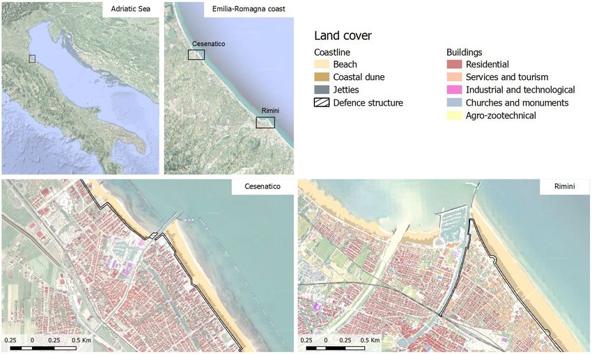
266                                                                M. Amadio et al.: CBA of coastal flood defence measures

bognin et al., 2009, 2010; Kirezci et al., 2020). Changes in       driven mainly by the astronomical tide, ranging about 1 m
the frequency of extreme events are likely to make existing        in the northernmost sector, and by meteorological forcing,
coastal protection inadequate in many places, causing a large      such as low pressure, seiches and prolonged rotational wind
part of European coasts to be exposed to flood hazard. Un-         systems, which are the main trigger of storm surge (Vous-
der these premises, coastal floods threaten to trigger devas-      doukas et al., 2017; Umgiesser et al., 2020). In addition to
tating impacts on human settlements and activities (McInnes        that, the whole coastal profile of the Padan plain shows rel-
et al., 2003; Lowe et al., 2001; Vousdoukas et al., 2017). In      atively fast subsiding rates, partially due to natural phenom-
this context, successful coastal risk mitigation and adaptation    ena but in large part linked to human activities (Perini et al.,
actions require accurate and detailed information about the        2017; Carbognin et al., 2009; Meli et al., 2020). As a con-
characterization of coastal flood hazard and the performance       tributing factor to coastal flood risk, the intensification of ur-
of coastal defence options. Cost–benefit analysis (CBA) is         banization has led to increased exposure along the Adriatic
widely used to evaluate the economic desirability of a disas-      coast during the last 50 years, with many regions building on
ter risk reduction (DRR) project (Jonkman et al., 2004; Price,     over half of the available land within 300 m of the shoreline
2018; Mechler, 2016), helping decision-makers in evaluating        (ISPRA, 2012). Figure 1 shows the location of the two case
the efficacy of different adaptation options (Kind, 2014; Bos      study areas, Cesenatico and Rimini, along with land-cover
and Zwaneveld, 2017).                                              maps showing the position of coastal defences accounted for
   In this study, we estimate the benefits of coastal renovation   in this study.
projects along the coast of the Emilia-Romagna region (Italy)         The number of ESL events reported to cause impacts along
in terms of avoided economic losses from ESL inundation            the Emilia-Romagna coast has shown a steady increase since
events under both current and future conditions. To do that,       the second half of the past century (Perini et al., 2011); this is
a range of hazard scenarios associated with ESL events are         partially explained by socio-economic development, which
simulated over the two case study areas: (i) Rimini, a touris-     has increased the extent of built-up assets potentially ex-
tic hotspot that is currently implementing a seafront reno-        posed to flood risk. The landscape along the 130 km regional
vation project, and (ii) Cesenatico, a coastal city that could     coastline is almost completely flat, the only relief being old
benefit from similar measures in addition to existing defence      beach ridges, artificial embankments and a small number of
mechanisms. The scenarios are designed by combining prob-          dunes. The coastal perimeter is delineated by a wide sandy
abilistic data from historical ESL events with the estimates       beach that is generally protected by offshore breakwaters,
of relative MSL change for those locations. Each scenario is       groins and jetties. The land elevation is often close to (or
evaluated in terms of direct economic impacts over residen-        even below) the MSL, and the coastal corridor is heavily ur-
tial areas using a flood damage model. The combination of          banized. Cesenatico has about 26 000 residents, while Rimini
different risk scenarios in a CBA framework allows the eval-       has 150 000. The towns are strongly touristic, hosting large
uation of the economic profitability brought by the project        beach resort and bathing facilities along the beach and with
implementation in terms of avoided losses up to the end of         hundreds of hotels and rental housing located just behind the
the century.                                                       beach. Both places have been affected by coastal storms, re-
                                                                   sulting in flooding of buildings and facilities, beach erosion,
                                                                   and regression of the coastline. The most recent inundation
2   Area of study                                                  events were observed in March 2010, November 2012 and
                                                                   February 2015. The 2015 event was one of the most severe
Located in the central Mediterranean Sea, the Italian penin-       ever recorded, with ESL values corresponding to a proba-
sula has more than 8300 km of coastline, hosting around            bility (return period) of once in 100 years. It caused severe
18 % of the country’s population, numerous towns and cities,       damage along the whole regional coast and, in some loca-
industrial plants, commercial harbours, and touristic activi-      tions, required the evacuation of people from their houses;
ties, as well as cultural and natural heritage sites. Existing     many buildings and roads were covered by sand brought by
country-scale estimates of SLR impacts up to the end of this       the flood wave; touristic infrastructures near the shore were
century help to identify the most critically exposed coastal       seriously damaged, and some port channels overflowed into
areas of Italy (Antonioli et al., 2017; Marsico et al., 2017;      the surrounding areas. The economic impact of the event was
Bonaduce et al., 2016; Lambeck et al., 2011). About 40 % of        estimated to top EUR 7.5 million (Perini et al., 2015).
the country’s coastal perimeter consists of a flat profile (IS-
PRA, 2012), potentially more vulnerable to the impacts of
ESL events. The North Adriatic coastal plain is the largest        3     Methodology
location and most vulnerable to extreme coastal events due
to the shape, morphology and low bathymetry of the Adri-           3.1    Components of the analysis
atic Sea basin, which cause the water level to increase rela-
tively fast during coastal storms (Perini et al., 2017; Ciavola    Coastal inundation is caused by an increase in the total water
and Coco, 2017; Carbognin et al., 2010). Here the ESL is           level (TWL), most often associated with extreme sea level

Nat. Hazards Earth Syst. Sci., 22, 265–286, 2022                                    https://doi.org/10.5194/nhess-22-265-2022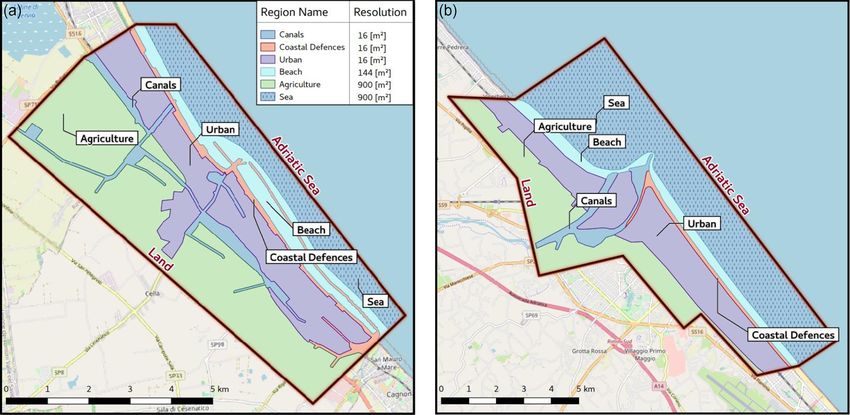
M. Amadio et al.: CBA of coastal flood defence measures                                                                              267

Figure 1. Case study locations along the Emilia-Romagna coast: Cesenatico and Rimini. The coastal defence structure assessed in this study
are shown in black. Buildings’ footprint data are from the Regional Environmental Protection Agency (ARPA) 2020. Basemap © Google
Maps 2020.

(ESL) events, which are often generated by a combination               and computationally quick, as it does not consider dynamic
of high astronomical tide and meteorological drivers such as           processes such as flow mass conservation and the effect of
storm surge and wind waves (Fig. 2). Probabilistic flood risk          land cover on the spread of floodwater, assuming flooded ar-
assessments generally consider ESL the result of the com-              eas to be those with an elevation below a forcing water level
bined effects of storm surge and tides (Muis et al., 2015;             (Hinkel et al., 2010, 2014; Jongman et al., 2012b; Ramirez
Vousdoukas et al., 2017). More recent studies also account             et al., 2016; Vousdoukas et al., 2016; Muis et al., 2016).
for the effects of waves by either adding wave setup to the            These assumptions and simplifications often result in sub-
ESL or simulating the dynamics of breaking waves on the                stantial misestimation of flood extents compared to hydrody-
coast (Kirezci et al., 2020; Melet et al., 2020; Li et al., 2020;      namic flood modelling and observations (Bates et al., 2005;
Wang et al., 2021; Muis et al., 2020; Lionello et al., 2021;           Vousdoukas et al., 2016; Breilh et al., 2013; Ramirez et al.,
McInnes et al., 2009; Idier et al., 2019). In our study, we            2016; Seenath et al., 2016; Kumbier et al., 2019; Anderson
consider the TWL nearshore the result of the combination of            et al., 2018). To overcome these limitations, hydrodynamic
high tide, storm surge and action of waves, the latter com-            flood modelling approaches capable of accounting for the
bining wave setup (defined as the increase in mean sea level           effects of wind, waves, tide, current and river run-off can
at the shore that is caused by the loss of wave momentum in            be used (Barnard et al., 2019). The most advanced models
the surf zone) with the wave periodicity of incoming break-            can simulate atmospheric–ocean–land interactions from the
ing waves (which defines wave swash, i.e. the amplitude of             deep ocean to the coast with a satisfactory predictive skill
the time-varying elevation due to breaking waves along the             (Bates et al., 2005; Seenath et al., 2016; Vousdoukas et al.,
shore).                                                                2016; Lewis et al., 2013), at the costs of a more complex
   The identification of areas threatened by coastal flooding          model setup, extensive data requirements and significantly
from ESL events is often done by means of flood maps,                  longer computational times (Teng et al., 2017). As an in-
which are generated through hydrostatic or hydrodynamic                termediate solution, simplified hydrodynamic flood models
modelling approaches. These approaches differ substantially            that focus on nearshore processes are capable of reducing
in their complexity and their ability to represent environmen-         the computational cost while taking into consideration wa-
tal processes. The hydrostatic inundation approach (some-              ter mass conservation (Breilh et al., 2013), aspects of flood-
times referred to as “bathtub”) is methodologically simple             ing hydrodynamics (Dottori et al., 2018) and the presence of

https://doi.org/10.5194/nhess-22-265-2022                                        Nat. Hazards Earth Syst. Sci., 22, 265–286, 2022
268                                                                    M. Amadio et al.: CBA of coastal flood defence measures

Figure 2. Components of the analysis for extreme sea level events: total water level is the sum of the maximum tide, storm surge and wind
waves over mean sea level. Vertical land movement and sea level rise affect the mean sea level on the long run.

obstacles (Perini et al., 2016). They have proved to be reli-          medium-term phenomena, such as sediment loading and soil
able for coastal flooding applications, such as the simulation         compaction (Carminati and Martinelli, 2002; Lambeck and
of coastal flooding due to storm tide events (Ramirez et al.,          Purcell, 2005). The latter can greatly exacerbate geological
2016; Bates et al., 2005; Skinner et al., 2015; Smith et al.,          processes at a local scale (Wöppelmann and Marcos, 2012);
2012).                                                                 in particular, faster subsidence occurs in the presence of in-
   In this study, estimates of ESL components (storm surge,            tense anthropogenic activities such as water withdrawal and
tides and waves) are obtained for the North Adriatic up to             natural-gas extraction (Teatini et al., 2006; Polcari et al.,
the year 2100 by combining reference hazard scenarios de-              2018). Most of the peninsula shows a slow subsiding trend,
rived from the analysis of historical records (Perini et al.,          although with some local variability. An estimate of VLM
2011, 2016, 2017; Armaroli et al., 2012; Armaroli and Duo,             rates due to tectonic activity has been derived from stud-
2018) with regionalized projections of SLR (Vousdoukas et              ies conducted in Italy (Solari et al., 2018; Antonioli et al.,
al., 2017) and local vertical land movement (VLM) rates                2017; Marsico et al., 2017; Lambeck et al., 2011). The North
(Perini et al., 2017; Carbognin et al., 2009). On this ba-             Adriatic coastal plain shows the most intense long-term geo-
sis, four hypothetical ESL scenarios are designed, ranging             logical subsidence rates (about 1 mm yr−1 ), increasing north
from low intensity–high frequency to high intensity–low fre-           to south. Yet in the last few decades these rates have of-
quency, under both current and future (2050 and 2100) con-             ten been greatly exceeded by ground compaction rates ob-
ditions. The hydrodynamic model ANUGA (Roberts et al.,                 served by remote sensing (Gambolati et al., 1998; Antonioli
2015) is applied to simulate the inundation of land areas dur-         et al., 2017; Polcari et al., 2018; Solari et al., 2018). Ob-
ing periods of ESL, accounting for individual components.              served subsidence is about 1 order of magnitude faster where
The land morphology and exposure of coastal settlements                the aquifer system has been extensively exploited for agri-
are described by high-resolution digital terrain model (DTM)           cultural, industrial and civil use since the post-war industrial
(lidar) and bathymetry, in combination with land use and               boom. Since the 1970s, however, with the halt of ground-
building footprints. The effect of hazard mitigation struc-            water withdrawals, anthropogenic drivers of subsidence have
tures (both designed and under construction) are explicitly            been strongly reduced or stopped (Carbognin et al., 2009).
accounted for by the model in the “defended” scenario, in              Nonetheless, subsidence still continues at much faster rates
contrast to the baseline scenario, where only existing defence         than expected from natural phenomena (Teatini et al., 2005).
structures (groins, jetties, breakwaters and sand dunes) are           Geodetic surveys carried out from 1953 to 2003 along the
considered.                                                            Ravenna coast provide evidence of a cumulative land sub-
                                                                       sidence exceeding 1 m at some sites due to gas extraction
3.2   Vertical land movement                                           activities. Average subsidence rates observed for 2006–2011
                                                                       along the Emilia-Romagna coast are around 5 mm yr−1 , ex-
Vertical land movements result from a combination of slow              ceeding 10 mm yr−1 on the backshore of the Cesenatico and
geological processes, such as tectonic activity and glacial            Rimini areas and topping 20–50 mm yr−1 in Ravenna (Perini
isostatic adjustment (Peltier et al., 2015; Peltier, 2004), and        et al., 2017; Carbognin et al., 2009). Based on these current

Nat. Hazards Earth Syst. Sci., 22, 265–286, 2022                                        https://doi.org/10.5194/nhess-22-265-2022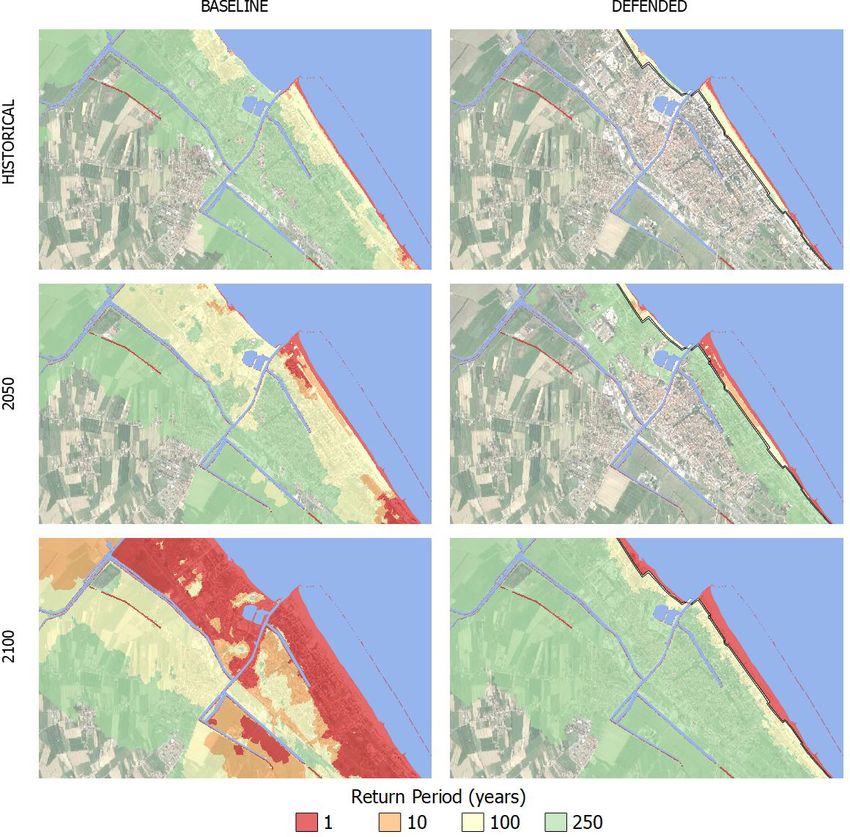
M. Amadio et al.: CBA of coastal flood defence measures                                                                      269

rates, we assume an average fixed annual VLM of 5 mm in           1946 to 2010 on the Emilia-Romagna (ER) coast, with half
both Cesenatico and Rimini up to the end of the century. This     of them causing severe impacts along the whole coast and
remarkable difference between natural VLM rates and ob-           10 of them being associated with important flooding events
servations would produce a dramatic effect on the estimated       (Perini et al., 2017). The most severe events are found when
SLR scenarios: at present rates, Rimini would see an increase     strong winds blow during exceptional tide peaks, most often
in the MSL by 0.15 m in 2050 and more than 0.4 m in 2100          happening in late autumn and winter. The event of Novem-
independently from eustatic SLR. Since these rates are con-       ber 1966 represents the highest ESL on record, causing sig-
nected with human activity, it is not possible to foresee how     nificant impacts along the regional coast: the recorded water
they will change in the longer run.                               level was 1.20 m a.m.s.l., and wave heights offshore were es-
                                                                  timated at around 6–7 m (Garnier et al., 2018; Perini et al.,
3.3   Sea level rise                                              2011). The whole coastline suffered from erosion and inun-
                                                                  dation, especially in the province of Rimini. Atmospheric
The long-term availability of tide gauge data along the           forcing has shown significant variability for the period of
North Adriatic coast allows an assessment of the changes in       1960 onwards (Tsimplis et al., 2012), but there is no strong
MSL during the last century, estimated to be +1.3 mm yr−1         evidence supporting a significant change in marine stormi-
(Scarascia and Lionello, 2013). This is consistent with pub-      ness frequency or severity for the near future (Lionello, 2012;
lished values for the Mediterranean Sea (Tsimplis et al.,         Zanchettin et al., 2020; Lionello et al., 2020, 2017). Thus, in
2008; Tsimplis and Rixen, 2002) and the Adriatic Sea (Tsim-       our model we assume meteorological forcing to remain the
plis et al., 2012; Carbognin et al., 2009). The projections of    same up to 2100.
future MSL account for sea thermal expansions from four
global circulation models, estimated contributions from ice       3.5   Terrain morphology and coastal defence structures
sheets and glaciers (Hinkel et al., 2014), and long-term sub-
sidence projections (Peltier, 2004). The ensemble mean is         Reliable bathymetry and topography are required in order to
chosen to represent each RCP for different time slices. The       run the hydrodynamic modelling at the local scale. Bathy-
increase in the central Mediterranean basin is projected to be    metric data for the Mediterranean Sea were obtained from the
approximately 0.2 m by 2050 and between 0.5 and 0.7 m by          European Marine Observation and Data Network (EMOD-
2100, compared to the historical mean (1970–2004) (Vous-          net) at a 100 m resolution. The description of terrain mor-
doukas et al., 2017). As agreed with local stakeholders (Co-      phology comes from the official high-resolution lidar DTM
mune di Rimini), our analysis considers the intermediate          (MATTM, 2019). First, we combine the coastal dataset (2 m
emission scenario RCP4.5, projecting an increase in the MSL       resolution and vertical accuracy of ±0.2 m) and the inland
of 0.53 m in 2100. It must be noted that these projections, al-   dataset (1 m resolution and vertical accuracy ±0.1 m) into
though downscaled for the Adriatic basin, do not account for      one seamless layer. Then, the DTM is supplemented with
the peculiar continental characteristics of the shallow north-    geometries of existing coastal protection elements such as
ern Adriatic sector, where the hydrodynamics and oceano-          jetties, groins and breakwaters obtained from the digital re-
graphic parameters partially depend on the freshwater inflow      gional technical map. In Rimini, the Parco del Mare (Fig. 3)
(Zanchettin et al., 2007).                                        is an urban renovation project which aims to improve the
                                                                  seafront promenade: the existing road and parking lots are
3.4   Tides and meteorological forcing                            converted into an urban green infrastructure consisting of
                                                                  a concrete barrier covered by vegetated sandy dunes with
Storm surge and wind waves represent the largest contribu-        walking paths. This project also acts as a coastal defence sys-
tions to the TWL during an ESL event. An estimation of            tem during extreme sea level events. The barrier rises 2.8 m
these components is obtained for the two coastal sites from       along the southern section of the town, south of the marina;
the analysis of tide gauge and buoy records and from the de-      no barrier is planned on the northern coastal perimeter. The
scription of historical extreme events presented in local stud-   Parco del Mare project is expected to be completed by 2022
ies (Armaroli and Duo, 2018; Perini et al., 2012; Masina et       and has been taken into account in the evaluation of the de-
al., 2015; Perini et al., 2011, 2017). This area is microtidal:   fended scenarios by adding the barrier elevation to the DTM.
the mean neap tidal range is 30–40 cm, and the mean spring           In Cesenatico, the existing defence structures include a
tidal range is 80–90 cm. Most storm surge events have a dura-     moving barrier system (Porte Vinciane) located in the port
tion of less than 24 h and a maximum significant wave height      channel, coupled with a dewatering pump which discharges
of about 2.5 m. During extreme cyclonic events, the sequence      the meteoric waters into the sea. The barriers close automat-
of SE wind (sirocco) piling the water north and ENE wind          ically if the TWL surpasses 1 m over the mean sea level,
(bora) pushing waves towards the coast can generate severe        preventing floods in the historical centre for up to 2.2 m
inundation events, with the significant wave height ranging       of TWL. Additional defence structures include the win-
3.3–4.7 m and exceptionally exceeding 5.5 m (Armaroli et          ter dunes, which consist of a 2.2 m tall intermittent, non-
al., 2012). Fifty significant events have been recorded from      reinforced sand barrier. In the defended scenario, we envis-

https://doi.org/10.5194/nhess-22-265-2022                                  Nat. Hazards Earth Syst. Sci., 22, 265–286, 2022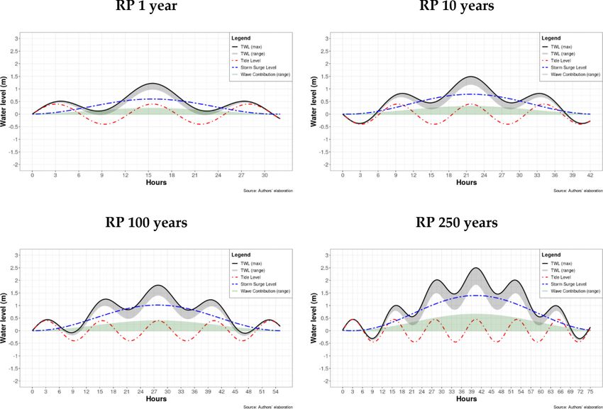
270                                                                   M. Amadio et al.: CBA of coastal flood defence measures

Figure 3. Prototype design of Parco del Mare project in Rimini. Adapted from JDS Architects.

age a coastal defence structure similar to Rimini’s Parco del         analysis concepts to characterize the amplitude and period
Mare project, spanning both north and south of the port chan-         of tidal, storm surge and wave levels as the harmonic con-
nel with a total length of 7.8 km. The DTM was manually               stituents that describe the theoretical temporal evolution of
edited based on additional reference data (i.e. on-site obser-        the nearshore TWL during an ESL event (see Fig. 4). Har-
vations or aerial photography) in order to remove artefacts           monic constituents are the elements in a mathematical ex-
and to produce a more realistic representation of the land            pression of a series of periodic terms and have been used
morphology. Bridges and tunnels are the most critical ele-            in harmonic analysis for sea level prediction (Boon, 2011;
ments that required DTM correction in order to avoid mis-             Familkhalili et al., 2020; Fuhrmann et al., 2019; Annunzi-
representations of the water flow routing.                            ato and Probst, 2016). The set of equations used in the study
                                                                      is specified in Appendix A, together with sample applica-
3.6   Scenario design                                                 tions and validation metrics of observed ESL events along
                                                                      the coast of ER. Additional variables to characterize the event
In order to design probabilistic nearshore scenarios associ-          dynamics are the storm surge duration (time, in hours) and
ated with ESL of different intensities to use as boundary con-        the wave period (Wp , in seconds), both obtained from re-
ditions in the hydrodynamic model, we rely on existing anal-          gional studies of ESL events (Armaroli et al., 2012; Armaroli
ysis of ESL events occurring on the regional coast (Perini            and Duo, 2018). Projections of the TWL at 2050 and 2100
et al., 2011, 2016, 2017), which have been adopted by the             are calculated for the same set of RP scenarios by adding
Regional Environmental Protection Agency to define the of-            SLR and VLM contributions to the MSL, thus shifting the
ficial coastal flood hazard zones and related protection stan-        TWL curve up by 33 cm in 2050 and by 97 cm in 2100.
dards (ARPA Emilia-Romagna, 2019). The probability of oc-                Figure 5 shows how the nearshore TWL results at any
currence of these ESL scenarios is expressed in terms of the          given time from the combination of the storm surge, tide level
return period (RP), which is the estimated average time inter-        and wave contribution in the scenario of RP 10 years (addi-
val (in years) between events of similar intensity. Four sce-         tional figures for all RP scenarios can be found in Appendix
narios of increasing intensity are designed, namely RP 1, 10,         A). The individual contribution of SS and Tmax levels are
100 and 250 years. For each of these hypothetical scenar-             represented by coloured dashed lines in the figure. The Wc
ios, the TWL nearshore is calculated as the sum of extreme            component is shown as a green-shaded area due to its high
values for the storm surge (SS) level, max tide (Tmax ) and           frequency (defined by the wave period, Wp , in seconds), thus
wave contribution (Wc ) at each time step (see Table 1). In           representing the range of values assumed at any given time.
particular, given the limitation of the considered 2D hydro-          The intensity of the wave contribution to the ESL is assumed
dynamic model in not resolving vertical convection and wave           to grow proportionally to the increase in the SS component.
breaking (i.e. swash), we include the wave contribution to the        The shaded grey area represents the range of the TWL as a
TWL by accounting for wave setup (Ws ) with a periodicity             sum of these components, while the solid black line repre-
equal to the incoming breaking waves (Wp ), thus partially            sents the maximum TWL at any given time. Our approach is
representing wave motion (Armaroli et al., 2012, 2009). We            precautionary as it provides worst-case TWL values: the SS
develop a set of trigonometric equations based on harmonic

Nat. Hazards Earth Syst. Sci., 22, 265–286, 2022                                       https://doi.org/10.5194/nhess-22-265-2022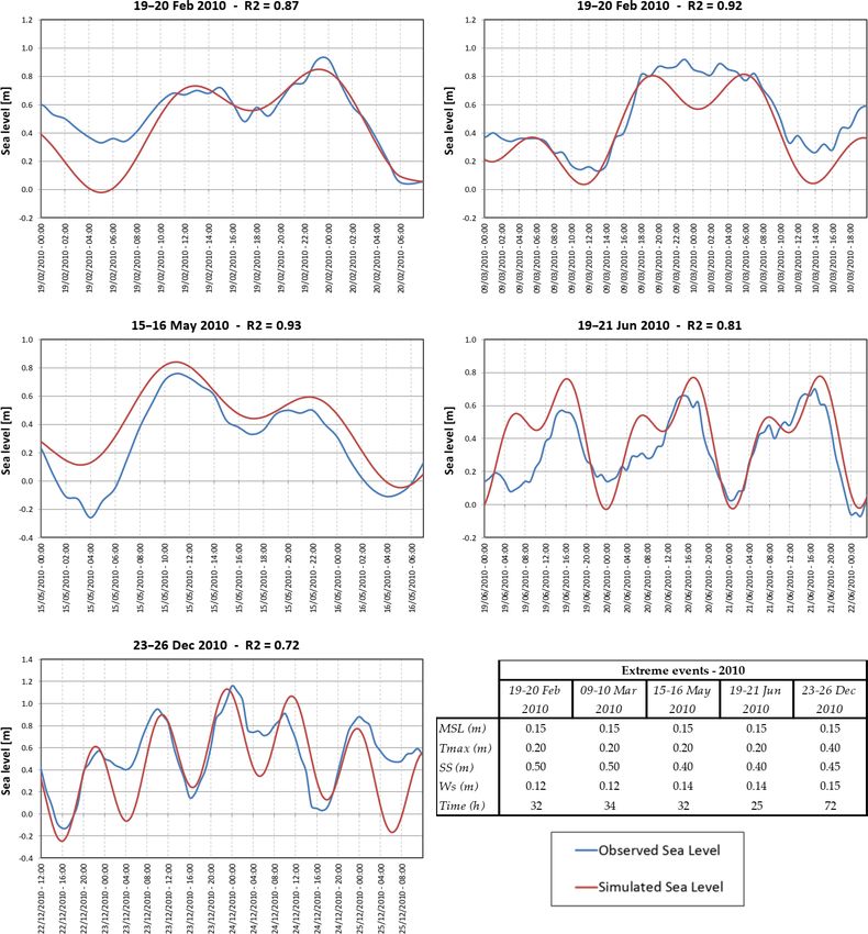
M. Amadio et al.: CBA of coastal flood defence measures                                                                                  271

Table 1. Components of nearshore TWL for four ESL scenarios (RPs) designed according to analysis of historical ESL events and projected
MSL change (2050 and 2100), accounting for both SLR (RCP4.5) and the average VLM rate.

                                Extreme event features           Historical            2050                      2100
              RP           SS    Tmax      Ws    Time     Wp         TWL      SLR     VLM      TWL      SLR     VLM      TWL
              (years)     (m)     (m)     (m)      (h)    (s)         (m)      (m)     (m)      (m)      (m)     (m)      (m)
              1          0.60    0.40    0.22       32    7.7         1.22    0.14     0.19     1.55    0.53     0.44     2.19
              10         0.79    0.40    0.30       42    8.9         1.49    0.14     0.19     1.82    0.53     0.44     2.46
              100        1.02    0.40    0.39       55    9.9         1.81    0.14     0.19     2.14    0.53     0.44     2.78
              250        1.40    0.45    0.65       75     11         2.50    0.14     0.19     2.83    0.53     0.44     3.47

Figure 4. Design of dynamic ESL scenario corresponding to RP 10 years under historical MSL conditions. The maximum TWL is shown
as the solid black line, while the TWL range at any given time is shown as the shaded grey area. The components of the nearshore TWL are
the tide level (dashed red line), the storm surge level (dashed blue line) and the wave contribution (green-shaded area). Wave contribution is
represented as a shaded area due to its high frequency (period of 8.9 s). In this scenario (RP 10) the maximum storm surge level is 0.79 m,
the maximum high tide is 0.40 m and the wave contribution ranges from 0.00 to 0.30 m, with a wave period of 8.9 s. At the peak of the event,
these conditions produce a maximum TWL of 1.49 m.

peak is set to coincide with Tmax and Wc at the middle of the            ity); thus it cannot account for the swash component of wave
event, thus resulting in the maximum TWL possible under                  runup. The wave direction is set to be oriented perpendicu-
each scenario.                                                           larly to the coast. For each scenario, ANUGA computes the
                                                                         TWL on the coast, the resulting water depth of inundation
3.7   Inundation modelling                                               and the horizontal momentum on an unstructured triangu-
                                                                         lar grid (mesh) representing the two case study areas. The
                                                                         size of the triangles is variable within the mesh, thus allow-
The nearshore ESL scenarios specified in Table 1 and ex-
                                                                         ing for a better representation in regions of particular inter-
emplified in Fig. 4 (and Appendix A) are used as forcing
                                                                         est, such as along the coastline, in urban areas and inside
boundary conditions in ANUGA, a 2D hydrodynamic model
                                                                         the canals. Six different regions are used in each case study
suitable for the simulation of flooding resulting from river-
                                                                         to define different triangular mesh resolutions, varying from
ine peak flows and storm surges (Roberts, 2020). The fluid
                                                                         higher-resolution areas of 16 m2 for canals and coastal de-
dynamics simulation is based on a finite-volume method for
                                                                         fence structures to a lower resolution of 900 m2 for sea areas.
solving the shallow-water wave equations, thus being based
                                                                         The output of the simulation consists of maps representing
on continuity and a simplified momentum equation. Being
                                                                         the flood extent, water depth and momentum at every time
a 2D hydrodynamic model, ANUGA does not resolve verti-
                                                                         step (∼ 1 s), projected onto the high-resolution DTM grid
cal convection, wave breaking or 3D turbulence (i.e. vortic-

https://doi.org/10.5194/nhess-22-265-2022                                            Nat. Hazards Earth Syst. Sci., 22, 265–286, 2022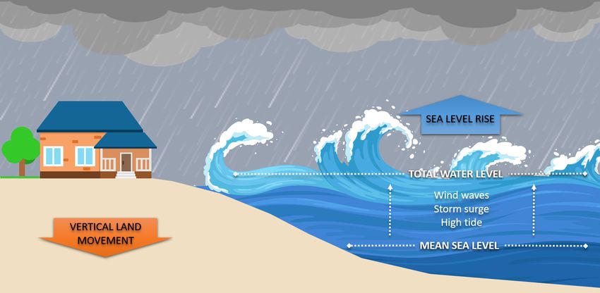
272                                                                   M. Amadio et al.: CBA of coastal flood defence measures

Figure 5. The definition of the simulation domain for the cities of Cesenatico (a) and Rimini (b). The legend shows the mesh resolution
specific to each region simulated by the model.

(1 m). Figure 6 presents the two case study areas and the re-         obtained from cadastral estimates (CRESME, 2019). The as-
spective resolutions for each region. The resulting irregular         set representation is static, thus not accounting for changes in
mesh contains about 637 000 triangles for the Cesenatico do-          land use or population density while allowing for the direct
main and about 1.2 million triangles for the Rimini domain.           comparison of hazard mitigation options’ results. A depth–
The model includes an operator module that simulates the              damage function validated on empirical records (Amadio et
removal of sand associated with the overtopping of a sand             al., 2019) is applied in order to translate each hazard scenario
dune by sea waves. The operator simulates the erosion, col-           into an estimate of economic risk, measured as a share of
lapse, fluidization and removal of sand from the dune system          the total exposed value. The damage function applies only to
(Kain et al., 2020). This option is enabled only in the unde-         residential and mixed residential buildings, the area of which
fended scenario for Cesenatico, where non-reinforced sand             represents about 93 % of the total exposed footprints; other
dunes are prone to erosion.                                           types (such as harbour infrastructures, industrial, commer-
                                                                      cial, historical monuments and natural sites) are excluded
3.8   Risk modelling and expected annual damage                       from risk computation. Abandoned or under-construction
                                                                      buildings are also excluded from the analysis. To avoid over-
Direct damage to physical assets is estimated using a custom-         counting of marginally affected buildings, we set two thresh-
ary flood risk assessment approach originally developed for           old conditions for damage calculation: the flood extent must
fluvial inundation, which is adapted to coastal flooding as-          be greater than or equal to 10 m2 and maximum water depth
suming that the dynamics of impact from long-setting floods           must be greater than or equal to 10 cm. The damage and prob-
depends on the same factors, namely (1) hazard magnitude              ability scenarios are combined together as expected annual
and (2) the type, size and value of the exposed asset. Indirect       damage (EAD). EAD is the damage that would occur in any
economic losses due to secondary effects of damage (e.g.              given year if damage from all flood probabilities were spread
business interruption) are excluded from the computation.             out evenly over time; mathematically, EAD is the integration
The hazard magnitude can be defined by a range of variables,          of the flood risk density curve over all probabilities (Olsen et
but the most important predictors of damage are water depth           al., 2015), as in Eq. (1).
and the extent of the flood event (Jongman et al., 2012a;
Huizinga et al., 2017). The characterization of the exposed                   Z1
asset is built from a variety of sources, starting from land          EAD =        D (p) dp                                        (1)
use and building footprints obtained from the regional en-
vironmental agencies’ geodatabases and the OpenStreetMap                       0

database (Open Street Map data for Nord-Est Italy, 2019).                The integration of the curve can be solved either analyt-
Additional indicators about building characteristics are ob-          ically or numerically, depending on the complexity of the
tained from the database of the 2011 Italian Census (15◦ cen-         damage function D(p). Several different methods for numer-
simento della populazione e delle abitazioni, 2019), while            ical integration exist; we use an approach where EAD is the
mean construction and restoration costs per building type are         sum of the product of the fractions of exceedance probabil-

Nat. Hazards Earth Syst. Sci., 22, 265–286, 2022                                       https://doi.org/10.5194/nhess-22-265-2022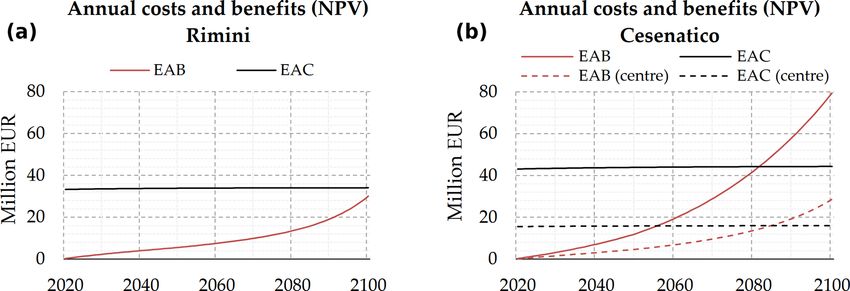
M. Amadio et al.: CBA of coastal flood defence measures                                                                            273

                                                                       di Rimini, 2019a, b, 2020, 2021a, b), the total cost of the
                                                                       project (to be completed during 2021) is EUR 33.3 million,
                                                                       corresponding to EUR 5.55 million per kilometre. No infor-
                                                                       mation is available about maintenance costs of the project,
                                                                       but given the nature of the project (static defence with low
                                                                       structural fragility), we assume they will be rather small com-
                                                                       pared to the initial investment. Ordinary annual maintenance
                                                                       costs (EAC) are accounted as 0.1 % of the total cost of the
                                                                       project. The same costs are assumed for the hypothetical bar-
                                                                       rier in Cesenatico, resulting in an initial investment cost of
                                                                       EUR 43.3 million. Costs and benefits occurring in the future
                                                                       periods need to be discounted, as people put higher value
                                                                       on the present (Rose et al., 2007). This is done by adjust-
Figure 6. Schematic representation of the numerical integration of     ing future costs and benefits using an annual discount rate
the damage function D(p) with respect to the exponential proba-        (r). We chose a variable rate of r = 3.5 for the first 50 years
bility of the hazard events. Damage (y axis) represents the ratio of   and r = 3 from 2050 onwards (Lowe, 2008). A sensitivity
damage to the total exposed value estimated up to the most extreme     analysis of the discount rate is included in Appendix B. The
scenario (RP 250 years). Events with a probability of occurrence       three main decision criteria used in CBA for project evalua-
higher than once in a year are expected to not cause damage (grey      tion are the net present value (NPV), the benefit / cost ratio
area).
                                                                       (BCR) and the payback period. The NPV is the sum of ex-
                                                                       pected annual benefits (B) up to the end of the time horizon,
ities and their corresponding damage (Fig. 7). We calculate            discounted, minus the total costs for the implementation of
D(p), which is the damage that occurs at the event with prob-          the defence measure, which takes into account initial invest-
ability p, by using the depth–damage function for each haz-            ment plus discounted annual maintenance costs (C). In other
ard scenario. The exceedance probability of each event (p)             words, the NPV of a project equals the present value of the
is calculated based on an exponential function as shown in             net benefits (NBi = Bi − Ci ) over a period of time (Board-
Eq. (2).                                                               man et al., 2018), as in Eq. (3).
                                                                                                     n
                                                                                                          NBr

               −1                                                                                   X
p = 1−e        RP
                                                                (2)    NPV = PV(B) − PV(C) =                                       (3)
                                                                                                    t=0
                                                                                                        (1 + r)t
   Events with a high probability of occurrence and low in-
tensity (below RP 1 year) are not simulated as they are as-               A positive NPV means that the project is economically
sumed to not cause significant damage. This is consistent              profitable. The BCR is instead the ratio between the benefits
with the historical observations for the case study area, al-          and the costs; a BCR larger than 1 means that the benefits of
though this assumption could change with increasing MSL.               the project exceed the costs in the long term and the project is
                                                                       considered profitable. The payback period is the number of
3.9   Cost–benefit analysis                                            years required for the discounted benefits to equal the total
                                                                       costs.
A CBA should include a complete assessment of the impacts
brought by the implementation of the hazard mitigation op-
tion, i.e. direct and indirect and tangible and intangible im-         4     Results
pacts (Bos and Zwaneveld, 2017). The project we are consid-
ering, however, has not been primarily designed for a DRR              4.1    Inundation scenarios
purpose; instead, it is meant as an urban renovation project
which aims to consolidate the touristic appeal of the area, to         Once the setup is completed, the hydrodynamic model per-
improve quality of life and the urban environment (Comune              forms relatively fast: each simulation is carried at half speed
di Rimini, 2018). This implies some large indirect effects on          compared to real time, requiring about 24 h to simulate a 12 h
the whole area, most of which are not strictly related to dis-         event. Parallel simulations for the same area can run on a
aster risk management and, overall, are very difficult to es-          multicore processor, improving the efficiency of the process.
timate ex ante. Our evaluation focuses only on the benefits            The output of the hydrodynamic model consists of a set of
that are measurable in terms of direct flood loss reduction.           inundation simulations that include several hazard intensity
Regarding the implementation costs, the CBA accounts for               variables in relation to flood extent: water depth, flow ve-
the initial investment required for setting up the adaptation          locity and duration of submersion. ESL scenarios are then
measure and operational costs through time. According to               summarized into static maps, each one representing the max-
the Parco del Mare project funding documentation (Comune               imum value reached by hazard intensity variables during the

https://doi.org/10.5194/nhess-22-265-2022                                        Nat. Hazards Earth Syst. Sci., 22, 265–286, 2022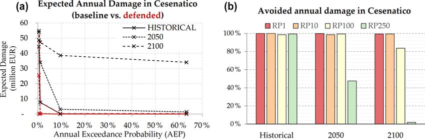
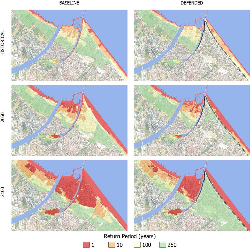
274                                                                      M. Amadio et al.: CBA of coastal flood defence measures

Figure 7. Rimini: extent of land affected by flood according to the frequency of occurrence of ESL events up to 2100 for the baseline (a) and
the defended (b) scenario. Basemap © Google Maps 2020.

simulated event at about a 1 m resolution. The flood extents             riers are enabled, the flood extent in the south-eastern urban
corresponding to each RP scenario are shown for Rimini                   area becomes almost zero for ESL events with a probability
(Fig. 8) and Cesenatico (Fig. 9).                                        of once in 100 years, even when accounting for SLR up to
   In Rimini, the Parco del Mare barrier produces benefits               2100. Under the most exceptional ESL conditions (RP 250
in terms of avoided flooding in the south-eastern part of the            in 2100), the barrier is overtopped, generating a flood extent
town (high-density area) for ESL events with a return period             similar to the baseline scenario for the same occurrence prob-
of 100 years or less. The north-western part and the marina              ability.
are outside of the defended area; these areas are therefore                 In Cesenatico, a barrier designed similarly to Parco del
subject to a similar amount of flooding across scenarios. In             Mare could provide significant reduction in flood extents un-
all the simulations, the buildings located behind the marina             der most hazard scenarios. Its effectiveness would be greater
are the first to be flooded. In fact, the new and the old port           than in Rimini thanks to the complementary movable bar-
channels located on both sides of the marina represent a haz-            rier system in use, which seals the port channel, allowing
ard hotspot: as shown in the maps, the failure of the east-              the walling off of the whole coastal perimeter and reducing
ern channel, which has a relatively low elevation, is likely to          the chance of water ingression in the urban area. In contrast,
cause the water to flood the eastern part of the town, even dur-         the erodible winter dune in the baseline defence scenario can
ing inundation events that would not surpass the beach. In the           only hold the heavy sea for shorter, less intense ESL events
defended scenarios, where both the coastal and the canal bar-            (RP 1–10 years) and becomes ineffective with more excep-

Nat. Hazards Earth Syst. Sci., 22, 265–286, 2022                                           https://doi.org/10.5194/nhess-22-265-2022
M. Amadio et al.: CBA of coastal flood defence measures                                                                             275

Figure 8. Cesenatico: extent of land affected by flood according to the frequency of occurrence of ESL events up to 2100 for the baseline
(a) and the defended (b) scenario. Basemap © Google Maps 2020.

Table 2. Summary of CBA for planned or designed seaside defence project in Rimini (all town and south section only) and Cesenatico (all
town and centre only) over a time horizon of 30 and 80 years (2021 to 2050 and 2021 to 2100).

                                                                     Rimini                           Cesenatico
                                                          All town            South only      All town         Centre only
            Metrics                                     2050     2100     2050       2100    2050   2100       2050     2100
            Baseline EAD (million EUR)                   2.8       32      0.5       14.6     1.7    25.9       0.5     12.4
            Defended EAD (million EUR)                   2.4       17      0.1        0.9     0.1     0.4       0.1      0.4
            Expected annual benefits (million EUR)       0.3       15      0.4       13.7     1.6    25.5       0.4     11.9
            Sum of EAB (discounted) (million EUR)        5.6       30      4.1       27.8    12.0    79.4       4.7     28.6
            Sum of EAC (discounted) (million EUR)       33.8     34.0     33.8       34.0    43.8    44.3      15.8     16.0
            Net present value (million EUR)            −28.3     −4.0    −29.8       −6.3   −31.8    35.1    −11.24     12.6
            Benefit / cost ratio (–)                    0.16     0.88     0.12       0.81    0.28    1.79      0.30     1.79

https://doi.org/10.5194/nhess-22-265-2022                                          Nat. Hazards Earth Syst. Sci., 22, 265–286, 2022
276 M. Amadio et al.: CBA of coastal flood defence measures
tional, long-lasting events; from 2050 on, the winter dune larger expected damage from increasing flood severity. The
could be surmounted and dismantled by sea waves even dur- cost of defence implementation is repaid by avoided dam-
ing non-exceptional events (RP 1 year). age after about 40 years in Cesenatico and after 90 years in
Rimini. In 2100, the BCR is 0.9 for Rimini and 1.8 for Cese-
4.2 Expected annual damage natico. These results clearly indicate an overall profitability
of the defence structure implementation over the long term
The expected annual damage is calculated as a function of for Cesenatico. For the case of the municipality of Rimini,
the maximum exposed value and water depth. In Rimini, further investigation is required in order to account for the
the EAD grows from around EUR 650 000 under histori- non-DRR benefits of the seafront renovation project. For in-
cal conditions to EUR 2.8 million in 2050 and more than stance, the potential reduction in indirect losses in terms of
EUR 32.3 million in 2100. Under less severe ESL scenar- capital and labour productivity due to less frequent and less
ios (RP below 100 years), the risk remains mostly confined intense flooding events and the potential increase in tourism
to around the marina, which is located outside the defended and well-being of citizens due to renewed urban landscape
area, producing expected damage below EUR 10 000. Under are factors that could be accounted for in a holistic CBA anal-
more extreme ESL scenarios, the benefits of the Parco del ysis and would likely return a shorter payback period.
Mare project protecting the southern part of Rimini become In order to better understand the potential benefits of the
more evident, avoiding about 65 % of the expected damage mitigation measures over different areas of the two munic-
in the defended scenarios compared to the undefended ones. ipalities, we compare the results in terms of the CBR over
The damage avoided in the defended scenarios grows almost a selection of exposed records corresponding to the towns’
linearly with the increase in the baseline EAD under future higher-density areas (i.e. Cesenatico historical centre, Rim-
projections of sea level rise: under the defended scenario, ini southern section). Table 2 summarizes the metrics of the
the EAD is reduced on average by 45 % in comparison with assessment for different area extent selections. CBA results
the undefended scenario (Fig. 10, left). The project produces do not differ much when considering different extents. In Ce-
benefits up to the scenario of RP 250 years in 2100, where a senatico benefits grow proportionally to costs, so the payback
projected TWL of 3.5 m would cause the overtopping of the time does not change when considering a section of the town
barrier, reducing the benefits to almost zero (Fig. 9, right). or the whole coastal perimeter.
In Cesenatico, the average EAD for the undefended sce-
nario grows from around EUR 270 000 under historical con-
ditions, to EUR 1.7 million in 2050 and almost EUR 26 mil- 5 Conclusions
lion in 2100. In our simulations, the designed defence struc-
ture (a static barrier with a height of 2.8 m along 7.8 km of In this study we addressed risk scenarios from coastal inun-
coast) is able to avoid most of the damage inflicted on res- dation over two coastal towns located along the North Adri-
idential buildings (Fig. 11, left). The measure becomes less atic coastal plain of Italy. This area is projected to become
efficient for the most extreme scenarios in 2050 and 2100, increasingly exposed to ESL events due to changes in MSL
when the increase in TWL causes the surmounting of the bar- induced by SLR and local subsidence phenomena. Both loca-
rier (Fig. 10, right). This assessment does not account for the tions are expected to suffer increasing economic losses from
impacts over those beach resorts and bathing facilities which these events, unless effective coastal adaptation measures are
are located along the barrier or between the barrier and the put in place. In order to understand the upcoming impacts
sea and thus are equally exposed in both the baseline and the and the potential benefits of designed coastal projects, first
defended scenario; they would likely represent an additional we designed probabilistic ESL scenarios based on local his-
7 %–25 % of the baseline damage. torical observations; then, we projected these scenarios to
2050 and 2100, accounting for the combined effect of SLR
4.3 Cost–benefit analysis and subsidence rates on the MSL. By using a high-resolution
hydrodynamic model, we produced flood hazard maps asso-
The estimates of avoided direct flood impacts are accounted ciated with each ESL scenario under both the baseline sce-
for in a DRR-oriented CBA to evaluate the feasibility of mit- nario and the defended hypothesis. The defended scenario
igation measures in terms of the NPV, BCR and payback accounts for the effect of a coastal barrier based on the de-
period for the two time horizons (for 2021–2050, 30 years; sign of Parco del Mare, an urban renovation project under
for 2021–2100, 80 years). The assessment does not measure construction in Rimini. The same type of defence structure is
the indirect benefits brought in terms of urban renovation, envisaged along the coastal perimeter of the nearby town of
which are the primary focus of the Parco del Mare project, Cesenatico. The hazard maps were fed to a locally calibrated
measuring, instead, only the direct benefits in terms of di- damage model in order to calculate the expected annual dam-
rect flood damage reduction. In Fig. 12, the expected an- age for both baseline and defended scenarios.
nual benefit (EAB) brought by defence measures grows at We run a CBA comparing expected damage in terms of
a faster rate approaching 2100 in both sites because of the flood losses over residential buildings, which represent the
Nat. Hazards Earth Syst. Sci., 22, 265–286, 2022 https://doi.org/10.5194/nhess-22-265-2022M. Amadio et al.: CBA of coastal flood defence measures 277 Figure 9. Rimini: expected annual damage (EAD) according to the undefended scenario up to 2100, all town considered (a); EAD reduction in the south-eastern part of the town thanks to hazard mitigation offered by the coastal barrier (b). Figure 10. Cesenatico: expected annual damage (EAD) according to the undefended scenario up to 2100 (a); EAD reduction thanks to hazard mitigation offered by the coastal barrier (b). Figure 11. Cumulated flood defence costs and expected benefits at the net present value for Rimini (a) and Cesenatico (b). https://doi.org/10.5194/nhess-22-265-2022 Nat. Hazards Earth Syst. Sci., 22, 265–286, 2022
278                                                               M. Amadio et al.: CBA of coastal flood defence measures

largest share of exposed buildings’ footprints (93 %). An in-     to match the peaks of tides and storm surge events) and t is
crease in damage is expected for both urban areas from 2021       the time in seconds.
to 2100: in Cesenatico the EAD grows by a factor of 96 and
                                                                                                    1
in Rimini by a factor of 49. The results show that the prof-      SS = SSmax × 0.5 × 1 + cos 2π        t + Sd + Sp     , (A2)
itability of present project investment grows over time in both                                    Sp
locations due to the increase in expected damage triggered by     where SS is the storm surge level in metres at any given time,
intense ESL events: the EAD under the baseline hypothesis         SSmax is the maximum storm surge level in metres, Sp is the
is expected to increase 3.5-fold in 2050 and up to 10-fold        storm surge duration in seconds, Sd is the storm surge shift in
in 2100. The benefits brought by the coastal defence project      time in seconds (used to match the peaks of tides and storm
become much larger in the second half of the century: the         surge events) and t is the time in seconds.
EAB grows 6.1-fold in Rimini and 6.5-fold in Cesenatico,
from 2050 to 2100. Avoided losses are expected to match the

                                                                                                 1
project implementation costs after about 40 years in Cesen-       Wc,int = 0.5 × 1 + cos 2π          t + Sd + Sp            (A3)
                                                                                                Sp
atico and 90 years in Rimini. Benefits are found to increase
                                                                                                      Wp

                                                                                               1
proportionally to costs; the payback period in Cesenatico is      Wc = Wmax × 0.5 × 1 + cos 2π     t+        × Wc,int        (A4)
                                                                                               Wp     4
the same considering an investment in the protection of either
the whole town or only part of it.                                   Where Wc is the wave contribution in metres at any given
   Further assessments of these renovation projects should        time, Wmax is the maximum wave setup level in metres, Wp is
look to measure the indirect and spillover effects on the lo-     the wave period in seconds, Wc,int is the intensity factor (0–
cal economy brought about by the project, possibly also ac-       1) of the wave contribution event as a function of the storm
counting for the intangible benefits and scenarios of exposure    surge intensity, Sp is the storm surge duration in seconds, Sd
change. The results are calculated in relation to emission sce-   is the storm surge shift in time in seconds (used to match the
nario RCP4.5; compared to RCP8.5 in 2050, the difference in       peaks of tides and storm surge events), and t is the time in
the SLR contribution is negligible (∼ 0.05 m), while in 2100,     seconds.
the difference between the two emission scenarios is larger          We consider the wave contribution component nearshore
(around 0.2 m); thus additional scenario analysis is suggested    as a function of the intensity of the storm surge level, as
to better address risk by the end of the century. On the haz-     shown in Eqs. (A3) and (A4). As such, the action of waves
ard modelling side, the particular consideration of combin-       is simulated as a composite function, where the maximum
ing wave setup and swash into a single wave contribution          wave contribution level is designed to coincide in time with
component can be considered theoretically questionable, as        the maximum storm tide level and the directions of the waves
wave setup is defined as the increase in mean sea level at        are set to coincide with the direction of the storm surge event,
the shore that is caused by the loss of wave momentum in          in our case, perpendicular to the coastline. This is done first
the surf zone, being often referred to as the static component    to follow the assumption of a worst-case scenario and second
of wave runup. For future works facing a similar challenge,       to incorporate the flood dynamics resulting from the momen-
we recommend accounting for the wave contribution to the          tum of waves directed inland. The composite function that
TWL as individual dynamic (i.e. swash) and static (runup)         combines Eqs. (A1) to (A4) and the effects of VLM and MSL
components.                                                       (e.g. due to SLR) is shown in Eq. (A5). The results of each
                                                                  component in Eqs. (A1) to (A4) and for each probabilistic
                                                                  scenario are shown in Fig. A1.
Appendix A
                                                                  TWL = MSL + VLM + Tl + SS + Ws                             (A5)
Here we present the equations and the graphical results of the
theoretical ESL scenarios. The TWL results from the com-             In order to verify the applicability of the aforementioned
bination of storm surge, tide and wave components, each           functions, we test the methods explained in this appendix for
following a general functional form (i.e. harmonic compo-         all five ESL events that were observed along the coastline
nent) describing the oscillation of the water level and follow-   of the ER region during the year 2010, as reported in Perini
ing trigonometric functional forms for each component. The        et al. (2011). Observed sea level data are obtained from IS-
equations are given as follows.                                   PRA, for the station Ravenna – Porto Corsini (Rete Mare-
                                                                  ografica Nazionale, 2021). We evaluate the goodness of fit

                   1
                                                                 of the methods by means of the coefficient of determination
Tl = Tmax × cos 2π    t + Td + Tp ,                       (A1)    (R 2 ). The results of this analysis are shown in Fig. A2.
                   Tp

where Tl is the tide level in metres at any given time, Tmax
is the maximum tide level in metres, Tp is the tidal period in
seconds, Td is the tidal period shift in time in seconds (used

Nat. Hazards Earth Syst. Sci., 22, 265–286, 2022                                   https://doi.org/10.5194/nhess-22-265-2022
M. Amadio et al.: CBA of coastal flood defence measures 279 Figure A1. Dynamic boundary conditions for simulating theoretical extreme sea level events in ANUGA. The total water level is shown as the grey-shaded area, while the maximum total water level is shown by the black line at any given time. The tide (dashed red line), storm surge (dashed blue line) and wave contribution (green-shaded area) components define the total water level. Configurations are shown for the return periods of once in 1, 10, 100 and 250 years. https://doi.org/10.5194/nhess-22-265-2022 Nat. Hazards Earth Syst. Sci., 22, 265–286, 2022
280                                                                    M. Amadio et al.: CBA of coastal flood defence measures

Figure A2. Comparison of the observed sea level (in blue) versus the simulated sea level using the harmonic components (in red).

Nat. Hazards Earth Syst. Sci., 22, 265–286, 2022                                         https://doi.org/10.5194/nhess-22-265-2022
M. Amadio et al.: CBA of coastal flood defence measures                                                                               281

Appendix B

A sensitivity analysis is carried out on the discount rate. Fig-
ure B1 shows how the NPV changes with the discount rate r
ranging from 1.5 % to 5.5 % (2020 to 2050) and 1 % to 5 %
(2050–2100).

Figure B1. Sensitivity analysis of NPV using a variable discount rate.

                                                                         Special issue statement. This article is part of the special issue
                                                                         “Coastal hazards and hydro-meteorological extremes”. It is not as-
Data availability. The geospatial data representing the modelled
                                                                         sociated with a conference.
inundation scenarios and the related risk output at the building level
are released on Zenodo (https://zenodo.org/record/4783443, Ama-
dio and Essenfelder, 2021).
                                                                         Acknowledgements. The research leading to this paper received
                                                                         funding through the projects CLARA (EU’s Horizon 2020 research
                                                                         and innovation programme under grant agreement 730482), Safer-
Author contributions. MA, AHE and SB conceptualized the study
                                                                         Places (Climate-KIC innovation partnership) and EUCP – the Eu-
and designed the experiments. AHE carried out the coastal haz-
                                                                         ropean Climate Prediction system – under grant agreement 776613.
ard modelling. SR advised on the model setup and calculation. SB
                                                                         We want to thank Luisa Perini for her kind support.
and PM provided required data and expertise about the case study
areas. MA performed the economic risk modelling and wrote the
manuscript. SM supported the CBA calculations. JM and SB man-
aged the funding acquisition and project supervision. All co-authors     Financial support. This research has been supported by Horizon
reviewed the manuscript.                                                 2020 (CLARA, grant no. 730482) and EIT Climate-KIC (Safer-
                                                                         Places) and EUCP – the European Climate Prediction system (grant
                                                                         agreement 776613).
Competing interests. The contact author has declared that neither
they nor their co-authors have any competing interests.
                                                                         Review statement. This paper was edited by Piero Lionello and re-
                                                                         viewed by two anonymous referees.
Disclaimer. Publisher’s note: Copernicus Publications remains
neutral with regard to jurisdictional claims in published maps and
institutional affiliations.

https://doi.org/10.5194/nhess-22-265-2022                                          Nat. Hazards Earth Syst. Sci., 22, 265–286, 2022
You can also read


