Radar sounding survey over Devon Ice Cap indicates the potential for a diverse hypersaline subglacial hydrological environment
←
→
Page content transcription
If your browser does not render page correctly, please read the page content below
The Cryosphere, 16, 379–395, 2022
https://doi.org/10.5194/tc-16-379-2022
© Author(s) 2022. This work is distributed under
the Creative Commons Attribution 4.0 License.

Radar sounding survey over Devon Ice Cap indicates the potential
for a diverse hypersaline subglacial hydrological environment
Anja Rutishauser1,2 , Donald D. Blankenship1,3 , Duncan A. Young1 , Natalie S. Wolfenbarger1 , Lucas H. Beem3 ,
Mark L. Skidmore3 , Ashley Dubnick4 , and Alison S. Criscitiello4
1 Institute
         for Geophysics, University of Texas at Austin, Austin, TX 78758, USA
2 GeologicalSurvey of Denmark and Greenland, Copenhagen, Denmark
3 Department of Earth Sciences, Montana State University, Bozeman, MT 59717, USA
4 Department of Earth and Atmospheric Sciences, University of Alberta, Edmonton, Alberta, Canada

Correspondence: Anja Rutishauser (rutishauser.anja@gmail.com)

Received: 15 July 2021 – Discussion started: 6 August 2021
Revised: 18 November 2021 – Accepted: 16 December 2021 – Published: 2 February 2022

Abstract. Prior geophysical surveys provided evidence for          ice cap (Burgess et al., 2005; Van Wychen et al., 2017; Pa-
a hypersaline subglacial lake complex beneath the center of        terson and Clarke, 1978) where basal ice temperatures are
Devon Ice Cap, Canadian Arctic; however, the full extent and       expected to be well below the pressure melting point of ice
characteristics of the hydrological system remained unknown        (Fig. 1). The brine-rich fluid of the lakes is hypothesized to
due to limited data coverage. Here, we present results from a      originate from the dissolution of a salt-bearing geological
new, targeted aerogeophysical survey that provides evidence        unit, referred to as the Bay Fiord Formation and abbreviated
(i) supporting the existence of a subglacial lake complex and      as Ocb (Harrison et al., 2016; Mayr, 1980; Thorsteinsson and
(ii) for a network of shallow brine/saturated sediments cover-     Mayr, 1987), which is projected to outcrop at the ice–bed in-
ing ∼ 170 km2 . Newly resolved lake shorelines indicate three      terface in the vicinity of the subglacial lakes (Rutishauser et
closely spaced lakes covering a total area of 24.6 km2 . These     al., 2018).
results indicate the presence of a diverse hypersaline sub-           The Devon subglacial lakes were inferred from radar
glacial hydrological environment with the potential to sup-        sounding measurements, a tool that has been widely used
port a range of microbial habitats, provide important con-         to characterize subglacial hydrological conditions (Carter et
straints for future investigations of this compelling scientific   al., 2007, 2009; Young et al., 2016; Palmer et al., 2013; Chu
target, and highlight its relevance as a terrestrial analog for    et al., 2018; Schroeder et al., 2015; Bowling et al., 2019).
aqueous systems on other icy worlds.                               However, the nature and full extent of the lakes and the sur-
                                                                   rounding hydrological conditions remained unresolved due
                                                                   to the relatively sparse data coverage. This motivated a tar-
                                                                   geted airborne geophysical survey over DIC where 4415 km
1   Introduction                                                   of profile lines were collected in dense survey grids (Fig. 1).
                                                                   Here, we use the resulting radar sounding measurements to
While numerous presumably freshwater subglacial lakes              evaluate the two features previously identified as subglacial
have been identified beneath the Antarctic (Siegert et al.,        lakes (Rutishauser et al., 2018), examine their full extents,
2016; Wright and Siegert, 2011) and Greenland ice sheets           and characterize the surrounding subglacial hydrological en-
(Palmer et al., 2013; Howat et al., 2015; Willis et al., 2015;     vironment. Our results support the previous interpretation for
Bowling et al., 2019), a recent study showed evidence for a        one of the subglacial lakes (Rutishauser et al., 2018) and in-
unique hypersaline subglacial lake complex beneath Devon           dicate large areas of wet bed consistent with projected salt-
Ice Cap (DIC), Canadian Arctic (Rutishauser et al., 2018).         bearing rock outcrops beneath the ice where the other lake
The features identified as subglacial lakes are situated in two    was identified (Rutishauser et al., 2018), which we inter-
bedrock troughs (T1 and T2) in the cold-based interior of the

Published by Copernicus Publications on behalf of the European Geosciences Union.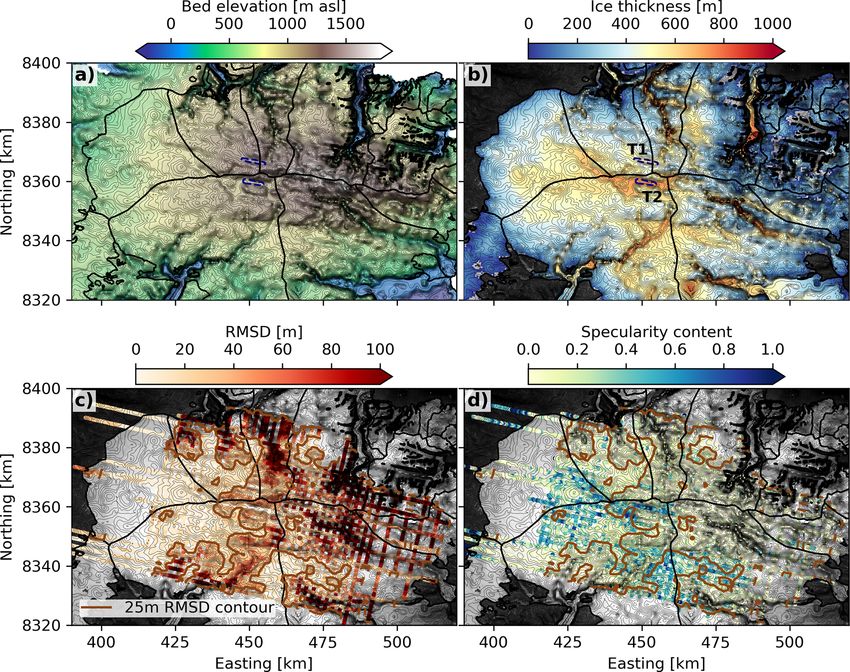
380                                                          A. Rutishauser et al.: Radar sounding survey over Devon Ice Cap

Figure 1. Map of Devon Ice Cap overlain with existing radar datasets collected prior to our survey (blue), including data presented in
Dowdeswell et al. (2004) and Rutishauser et al. (2016, 2018), as well as conducted in Operation IceBridge surveys between 2011–2015
(Paden et al., 2019), and the aerogeophysical survey profiles collected in this study (SRH1; red). Blue outlines mark the location of the
previously inferred subglacial lakes in bedrock troughs T1 and T2 (Rutishauser et al., 2018), and the thin black lines mark the boundaries
of the glacier catchment areas. Background image features the ArcticDEM surface elevation map by the Polar Geospatial Center from
DigitalGlobe Inc. imagery (Porter et al., 2018).

pret as a brine network rather than a lake. We estimate the            collected using the Multifrequency Airborne Radar-sounder
areal extent of the lakes and distributed brine network and            for Full-phase Assessment (MARFA) (Young et al., 2016),
model potential flow routes of the subglacial brine. Finally,          a dual-phase center version of the High Capability Airborne
subglacial hydrologic systems, both fresh and saline, have             Radar Sounder (HiCARS) system operated by the Univer-
been shown to harbor unique microbial ecosystems (Mikucki              sity of Texas Institute for Geophysics (UTIG). The radar is
and Priscu, 2007; Karl et al., 1999; Skidmore et al., 2005;            a coherent system with a 60 MHz center frequency and a
Christner et al., 2014; Boetius et al., 2015; Achberger et al.,        15 MHz bandwidth (2.8 m wavelength in ice). Detailed in-
2017) and have therefore long been considered as terrestrial           strument characteristics and processing techniques are de-
analogs for icy habitats on other planetary bodies (Cockell et         scribed in Peters et al. (2005, 2007). Additional science in-
al., 2011; Garcia-Lopez and Cid, 2017). Here, we discuss the           strumentation deployed during the SRH1 survey included a
microbial habitats that could be hosted in the diverse sub-            Novatel SPAN Inertial Navigation System for precise posi-
glacial environment beneath DIC and the relevance of this              tioning and orientation, a Riegl laser altimeter, a Cesium va-
system as a terrestrial analog for aqueous systems on other            por magnetometer, and a downward-looking Canon DSLR
icy worlds.                                                            camera. In this study, we present the radar sounding data
                                                                       and use unfocused synthetic-aperture radar (SAR) processed
                                                                       low-gain data to derive basal reflection coefficients, use 1-D
2   Data and methods                                                   focused SAR processed data (Peters et al., 2007) to identify
                                                                       the subglacial bedrock topography utilized in the bed digi-
Data used in this study were collected during an aerogeo-              tal elevation model (DEM) and basal roughness estimates,
physical campaign over DIC in spring 2018 (dataset referred            and combine 1-D and 2-D focusing to derive the specular-
to as SRH1), utilizing a Basler BT-67 (DC-3T) aircraft op-             ity content of the bed echo (Schroeder et al., 2013, 2015).
erated by Kenn Borek Air Ltd. as survey platform. A total              The nominal along-track trace spacing of the dataset is about
of 4415 km of along-track data was acquired in a grid survey           22 m with a vertical resolution of about 6 m in ice and an av-
with line spacing ranging from 1.25 to 5 km and the densest            erage pulse-limited footprint diameter at the glacier bed of
grid centered over the area of the previously inferred sub-            274 m.
glacial lakes (Fig. 1). Radar echo sounding (RES) data were

The Cryosphere, 16, 379–395, 2022                                                            https://doi.org/10.5194/tc-16-379-2022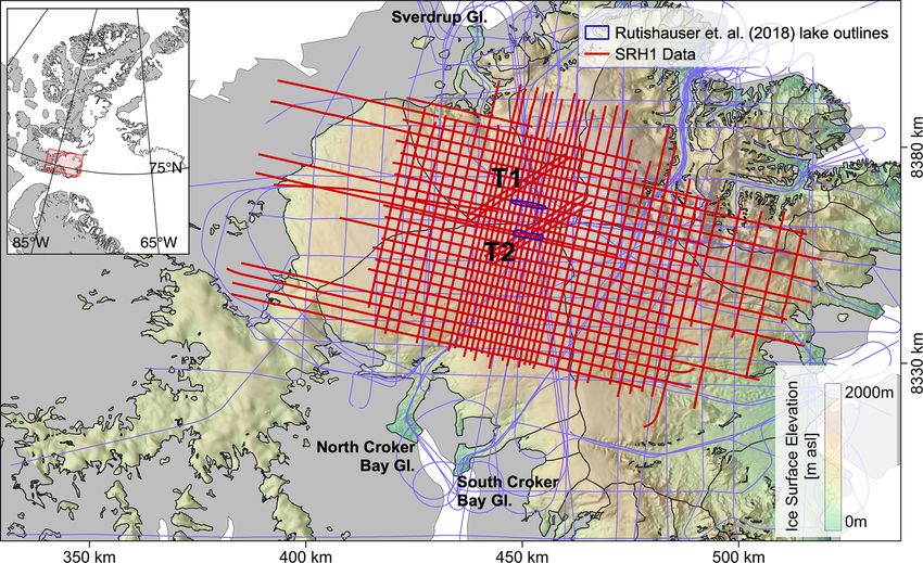
A. Rutishauser et al.: Radar sounding survey over Devon Ice Cap                                                                 381

2.1   Bedrock DEM                                                   material with high electrical conductivity (e.g., clay, brine-
                                                                    saturated sediments) can produce equally strong reflections
The DEM of the bed topography previously derived in                 as subglacial lakes filled with freshwater. Thus, it is impor-
Rutishauser et al. (2018) compiled RES data collected over          tant to consider both changes in water content and electrical
DIC by the Scott Polar Research Institute (SPRI) in 2000            conductivity when interpreting basal reflectivity. Bed reflec-
(Dowdeswell et al., 2004), HiCARS data collected in 2014            tivity values derived from radar measurements are also af-
(Rutishauser et al., 2016, 2018), and RES data from Oper-           fected by the characteristics of the radar system and atten-
ation IceBridge surveys between 2011–2015 (Paden et al.,            uation processes, and thus a number of corrections are re-
2019). Here, we update the previous bed DEM (1 km × 1 km            quired before basal reflectivity values can be interpreted in
grid mesh) using the SRH1 data as an additional dataset and         terms of subglacial hydrological conditions (Wolovick et al.,
produce a new DEM over a 500 m × 500 m grid mesh.                   2013; Chu et al., 2016; Schroeder et al., 2016; Matsuoka et
   The bed return from the SRH1 data is identified using a          al., 2010, 2012). Here, we derive the relative basal reflectivity
semi-automated picking algorithm, which locates the max-            (R) following
imum bed reflection power within manually defined depth
boundaries. Over the steep valley walls of bedrock trough T2,       [R]dB = [P ]dB + [B]dB + [G]dB + [L]dB − [S]dB ,             (1)
the basal reflection was discriminated from cross-track clut-
ter using the results from Scanlan et al. (2020). Travel times      where P is the returned bed power, B is the birefringence ef-
were then converted to depths using a radar wave velocity in        fects due to variations of the ice crystal fabric (Matsuoka et
ice of 168.4 m µs−1 .                                               al., 2003), G is the power loss from geometric spreading of
   Bed elevation data from all surveys over DIC described           the radar beam, L is the loss from englacial attenuation, and
above were interpolated over a 500 m grid mesh via ordi-            S is the correction for power variations in the radar system,
nary kriging to generate a new DEM. To ensure a continuous          where the notation []dB refers to the terms expressed in deci-
transition between the bed DEM and the non-glaciated sur-           bels ([X]dB = 10log10 (X)) (Matsuoka et al., 2012). Here, S
rounding topography, land elevations from the ArcticDEM,            is assumed to be constant as no changes were made to the
Polar Geospatial Center, and from DigitalGlobe Inc. imagery         radar instrument settings during the field campaign. Under
(Porter et al., 2018) outside of the ice cap were included in       the assumption of a relatively uniform pattern of crystal fab-
the bed DEM generation. A total of 47 233 crossover points          ric orientation over the survey area, we assume that birefrin-
reveal a mean crossover error of 0.1 m in nadir ice thickness       gence effects are relatively constant and thus neglect both
(mean absolute error of 17.6 m) with a standard deviation           terms S and B when analyzing relative basal reflectivity. The
of 46.0 m (Fig. S5 in the Supplement). Sources of errors in         power loss from geometric spreading of a specular echo is
the radar-derived bed elevation include uncertainties in the        derived from
ice surface due to a heterogeneous firn affected by melting–                             √
                                                                    [G]dB = 2 2 h + d/ ε dB ,                                  (2)
refreezing processes (Rutishauser et al., 2016) that are prop-
agated into the bed elevation, anisotropic cross-track scatter-     where h is the aircraft range above the glacier surface, d is
ing at the surface and bedrock (Scanlan et al., 2020), and          the ice thickness, and ε = 3.17 (Evans, 1965) is the dielec-
uncertainties in the velocity-to-depth conversion. A compar-        tric permittivity of ice (Schroeder et al., 2016). The englacial
ison of the bed DEM to the raw data shows that largest grid-        attenuation loss term L is related to the one-way depth-
ding errors appear in deep bedrock troughs connected to the         averaged attenuation rate N via
ice cap’s outlet glaciers and where the ice is thicker (Fig. S6
in the Supplement). These errors are likely caused by uncer-        [L]dB = 2N d .                                               (3)
tainties in the bedrock picks due to cross-track reflections at
the subglacial valley walls (Scanlan et al., 2020), a decreased     Attenuation rates were derived from a linear fit between
signal-to-noise ratio beneath thicker ice, and a rapidly chang-     the ice thickness and geometrically corrected bed reflection
ing bed topography over short distances not captured in our         power (Gades et al., 2000; Wolovick et al., 2013; Schroeder
grid.                                                               et al., 2016). We constrain our fit to ice thicknesses be-
                                                                    tween 50–650 m where the relationship appears most linear,
2.2   Basal reflectivity                                            resulting in a one-way attenuation rate (slope of the fit) of
                                                                    21.8 dB km−1 , with a correlation coefficient (R) of −0.57
Radar-derived measurements of basal reflectivity have been          (Fig. 2). The root-mean-square error (RMSE) between the
widely used to identify the presence of subglacial water (Ja-       regression line and the observed bed power is 8.0 dB, indi-
cobel et al., 2009; Peters et al., 2005; Chu et al., 2018; Carter   cating relatively large attenuation rate uncertainties. This is
et al., 2007). The basis for such interpretations is that an ice–   likely due to processes affecting the radar attenuation rate
water interface has a higher reflectivity than surrounding ar-      that are not accounted for in this simple regression method,
eas where ice is in direct contact with dry bedrock. How-           including the presence of subglacial water (increases the bed
ever, Tulaczyk and Foley (2020) demonstrate that subglacial         power for a given ice thickness), heterogeneous distribution

https://doi.org/10.5194/tc-16-379-2022                                                       The Cryosphere, 16, 379–395, 2022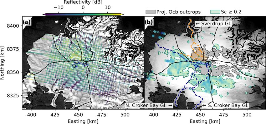
382                                                              A. Rutishauser et al.: Radar sounding survey over Devon Ice Cap

                                                                         ter (Oswald and Gogineni, 2012; Greenbaum et al., 2015;
                                                                         Rutishauser et al., 2018; Carter et al., 2007; Young et al.,
                                                                         2016) and characterize the configuration of subglacial hy-
                                                                         drological systems (Schroeder et al., 2013, 2015). However,
                                                                         we note that weak sediments or highly polished bedrock that
                                                                         has a flat and smooth interface on a wavelength scale could
                                                                         produce a similarly high specularity as an ice–water inter-
                                                                         face. The specularity has also been used to derive the fine-
                                                                         scale roughness of glacier beds (Jordan et al., 2017; Cooper
                                                                         et al., 2019), which has been related to the subglacial geology
                                                                         (Cooper et al., 2019).
                                                                            Here, we derive the specularity by comparing the re-
                                                                         turned peak energy from two different SAR focusing aperture
                                                                         lengths (1-D and 2-D focusing corresponding to 0.1 and 1 µs
                                                                         range delay, respectively) following Schroeder et al. (2015).
                                                                         To ensure the interpretation of subglacial water only over sig-
Figure 2. Derivation of englacial attenuation rates. Correlation and     nificantly large areas, we apply a running-mean filter to the
linear fit (red) between the ice thickness and the geometrically cor-    basal reflectivity and specularity over a 250 m window length
rected bed power of the SRH1 dataset over DIC, along with contour        along track, corresponding to just below the average pulse-
lines indicating the density distribution. The attenuation rate is de-   limited footprint at the glacier bed of our dataset.
rived from the slope of the fit (21.8 dB km−1 ).
                                                                         2.4   Basal roughness
of ice temperature and chemistry, and the ice surface and
bedrock roughness (decreases the bed power for a given ice               While the specularity content is a proxy for basal roughness
thickness). Here, we do not attempt to further constrain the             on a wavelength scale, we derive larger-scale basal roughness
variability in attenuation rates and use the 21.8 dB km−1 at-            via the root-mean-square deviation (RMSD) of the bedrock
tenuation rate to correct the observed bed power over the en-            topography along flight lines following Shepard et al. (2001).
tire dataset. The uncertainty of the measured basal reflectivity         We tested different lags (step sizes) between 50 and 1000 m
is estimated from the mean crossover error of the geometri-              over 5 km window lengths repeated at every bedrock obser-
cally corrected bed power values along the survey profiles,              vation, for which the resulting subglacial roughness pattern
which is 5.2 dB.                                                         does not change significantly. To show the distribution of the
   In this study, we do not derive absolute basal reflection co-         RMSD-derived subglacial roughness in this study, we choose
efficients but rather compare basal reflectivity in a relative           a lag of 500 m.
sense. To allow for an easier visual inspection of reflectiv-
ity anomalies that could suggest the presence of subglacial              2.5   Subglacial hydraulic head and water flow paths
water, we normalize the basal reflectivity by subtracting the
mean of all measured reflectivity values such that they are              We calculate the hydraulic head over a 500 m mesh grid
distributed around 0 dB (Fig. 4f).                                       following Shreve (1972) and described in Wolovick et al.
                                                                         (2013), using ice surface elevation derived from the Arctic-
2.3   Specularity content                                                DEM (Porter et al., 2018), the newly generated bed DEM,
                                                                         and a subglacial brine density of 1150 kg m−3 (correspond-
The specularity of the returned bedrock signal is governed               ing to a brine with 15 wt % NaCl; Rutishauser et al., 2018).
by scattering properties of the radar wave and is sensitive              To compute the hydraulic head for orthometric heights, the
to the interface roughness on a wavelength scale (Shepard                surface and bed elevation were corrected for gradients in the
and Campbell, 1999; Schroeder et al., 2015). The scatter-                geoid, using the Arctic Gravity Project geoid (Arctic Gravity
ing characteristics can be derived from the shape (i.e., pulse-          Project, 2006). Uncertainties of the hydraulic head are de-
peakiness/waveform abruptness) of the reflected waveform                 rived by propagating the standard deviation of the crossover
(Oswald and Gogineni, 2008, 2012; Jordan et al., 2017;                   errors in the bed elevation (46.0 m) and an estimated uncer-
Cooper et al., 2019) or as a function of the along-track an-             tainty of 3.7 m for the ArcticDEM (Supplement), resulting
gular distribution of the returned energy (Schroeder et al.,             in a total uncertainty of 12.3 m for the hydraulic head. To
2013; Young et al., 2016; Schroeder et al., 2015), the lat-              identify hydraulically flat areas, we derive the slope of the
ter of which we apply here. Ice–water interfaces that are                hydraulic head (tan ∇θ), which has an uncertainty of 1.4◦ .
flat on wavelength scales are expected to produce specular                  Potential flow paths for subglacial water are derived via
radar reflections (Schroeder et al., 2013, 2015), a character-           application of a flow accumulation algorithm by TopoTool-
istic that has previously been used to identify subglacial wa-           box (Schwanghart and Kuhn, 2010) to the hydraulic head dis-

The Cryosphere, 16, 379–395, 2022                                                            https://doi.org/10.5194/tc-16-379-2022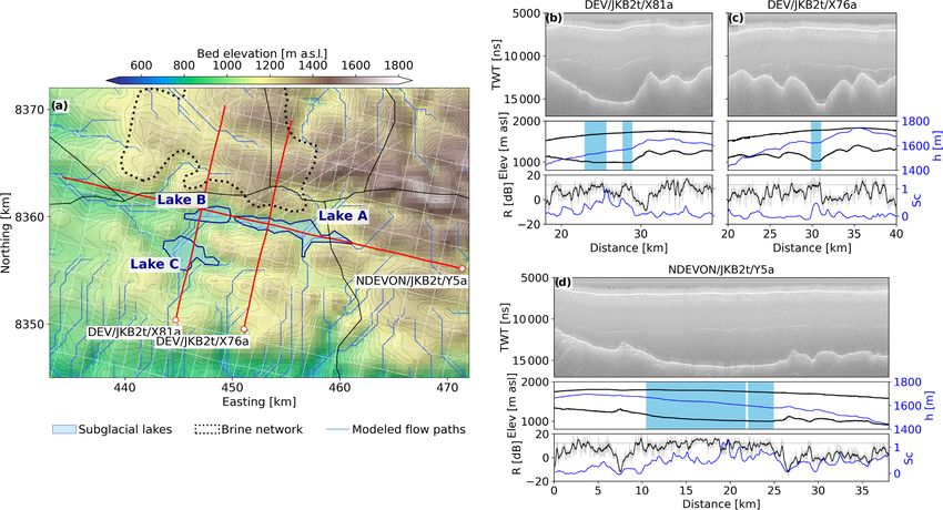
A. Rutishauser et al.: Radar sounding survey over Devon Ice Cap                                                                 383

tribution. In this algorithm flow paths are identified from all     and the lowlands can also be observed in the RMSD-derived
grid cells that drain a minimum of 10 upstream cells. Mod-          basal roughness (Fig. 3c) and the bed specularity content
eled subglacial flow paths are generally very sensitive to vari-    (Fig. 3d), which is a proxy for the small-scale roughness of
ations in the bed topography (MacKie et al., 2021). To ac-          the glacier bed (Young et al., 2016; Schroeder et al., 2013,
count for uncertainties in our bed DEM, the water routing           2015).
model is repeated 1000 times with randomly perturbed hy-
draulic heads by adding normally distributed errors with a          3.2   Distribution of subglacial water from radar
standard deviation equal to the hydraulic head uncertainty.               reflectivity
Additionally, to test the water routing model for potentially
larger uncertainties in the bed DEM towards the ice cap mar-        After all corrections are applied, relative basal radar reflec-
gins where data coverage is reduced, we apply errors equal          tivity values represent a combination of changes in the di-
to 2 and 3 times the hydraulic head uncertainty.                    electric permittivity (i.e., presence of water) and electrical
   A critical implication of a brine-rich subglacial fluid is the   conductivity (i.e., salinity, presence of clay) at the glacier
increase in relative importance of the bed versus ice surface       bed, as well as the roughness of the ice–bed interface (Pe-
topography on the hydraulic gradient as the density of the          ters et al., 2005; Tulaczyk and Foley, 2020). Although the
fluid increases – from ∼ 1/11 (bed/surface topography) for          smooth lowlands show elevated basal reflectivity in general,
freshwater to ∼ 1/4 for a subglacial brine with a density of        the highest magnitudes are concentrated in the western part
1150 kg m−3 (Rutishauser et al., 2018). Further, we note that       of the central massif (Fig. 4a). Excluding the effects of elec-
the model applied here does not capture spatially varying           trical conductivity of a subglacial material (Tulaczyk and Fo-
brine chemistry for example from changes in basal tempera-          ley, 2020), variations in basal reflectivity have typically been
ture (i.e., cryoconcentration of the brine), evolving drainage      interpreted as transitions between wet and dry bedrock con-
morphology through frictional heat dissipation or changes in        ditions (Chu et al., 2018; Hubbard et al., 2004; Christian-
effective water pressure, or other effects such as thermally        son et al., 2012; Peters et al., 2005; Carter et al., 2007; Chu
constrained (i.e., a cold-ice seal) pathways (Skidmore and          et al., 2016). Based on that, the observed reflectivity pat-
Sharp, 1999; Livingstone et al., 2012).                             tern suggests that widespread areas of wet bed lie beneath
                                                                    the central part of DIC. However, the observed variations
                                                                    in relative bed reflectivity could also result from changes in
3     Results                                                       electrical conductivity of the subglacial material (rather than
                                                                    dry–wet transitions), including changes in the salinity (e.g.,
3.1    Subglacial bedrock morphology                                freshwater versus brine) of subglacial water or saturated sed-
                                                                    iments (Tulaczyk and Foley, 2020). While some variations in
While large-scale terrain characteristics could be obtained         brine salinity likely occur, the existence of freshwater over
from previous bed DEMs (Dowdeswell et al., 2004;                    the study area is unlikely due to estimated basal ice temper-
Rutishauser et al., 2018), our dataset and the new, finer-          atures well below the pressure melting point (Fig. S7 in the
resolution DEM reveals additional features in the smaller-          Supplement; Burgess et al., 2005; Van Wychen et al., 2017;
scale terrain (Fig. 3a). This updated DEM shows that bedrock        Paterson and Clarke, 1978). Furthermore, we cannot rule out
trough T2, which was previously inferred to host a subglacial       that high-basal-reflectivity anomalies are caused by dry but
lake (Rutishauser et al., 2018), is part of a deeply (∼ 150–        highly conductive bed material (further detailed in the Dis-
300 m) incised canyon that likely extends toward the west-          cussion section). Nevertheless, we hereafter interpret high-
ern margin of the ice cap (Fig. 3a) and is overlain by ice          relative-reflectivity anomalies as areas consisting of saline
exceeding 700 m thickness in large portions of the canyon           subglacial water (brine) and in the form of saturated sed-
(Fig. 3b). This canyon is one of the most extensive features        iments. The theoretical contrast in Fresnel reflectivity be-
beneath DIC and, unlike other canyons, does not connect to          tween wet and dry beds is estimated to be about 10–15 dB
a marine-terminating outlet glacier under current ice dynam-        (Peters et al., 2005); however, the thresholds that have been
ics. In comparison to T2, trough T1 (previously inferred to         used in the literature to differentiate between subglacial wa-
host the other subglacial lake) is less incised (∼ 100–200 m)       ter and surrounding dry bedrock are highly variable, ranging
into the bedrock and widens towards a plateau area in the           between 2 and 26 dB (Wolovick et al., 2013; Carter et al.,
northwest, leading into a canyon headward from Sverdrup             2009; Oswald and Gogineni, 2008; Jacobel et al., 2010; Chu
Glacier.                                                            et al., 2016). Here, we use a threshold of 12 dB above the
   The interior part of DIC is underlain by mountainous ter-        mean of all observed reflectivity values in this study (1.5σ
rain (hereby referred to as “the central massif”), whereas the      reflectivity anomaly, Fig. 4f) to quantitatively identify poten-
southern and western parts of the ice cap (hereby referred          tial areas of subglacial water/brine (Fig. 4b), which is consis-
as “lowlands”) are characterized by relatively flat bed topog-      tent with the theoretical Fresnel reflectivity increase between
raphy, which is dissected by a few large glacial troughs in         a dry and wet bed for the dielectric permittivity of seawa-
the south. The general transition between the central massif        ter (Neal, 1979; Peters et al., 2005). Our results suggest the

https://doi.org/10.5194/tc-16-379-2022                                                      The Cryosphere, 16, 379–395, 2022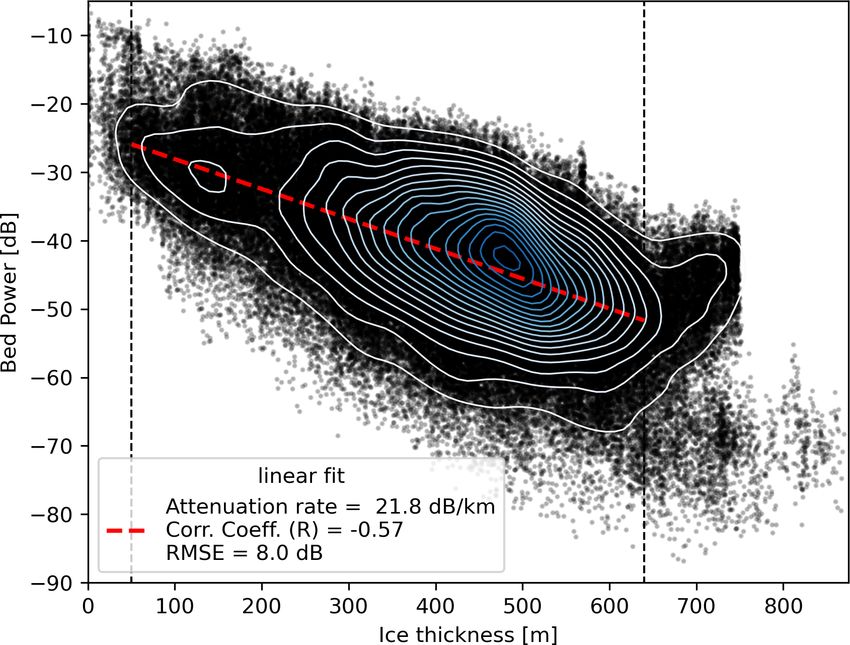
384 A. Rutishauser et al.: Radar sounding survey over Devon Ice Cap
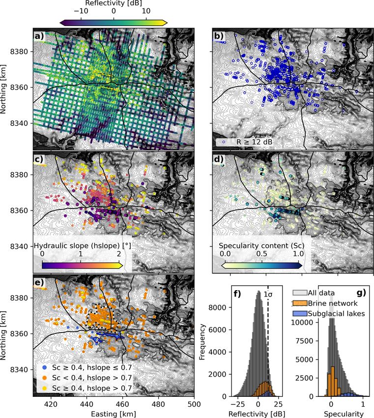
Figure 3. Subglacial bedrock morphology beneath DIC. (a) Updated bedrock DEM from this study with 25 m contour lines. Thick black lines
mark the boundaries of the glacier catchment areas. (b) Ice thickness derived via a subtraction of the bedrock DEM from the ArcticDEM ice
surface elevation (Porter et al., 2018). The location of the previously inferred subglacial lakes in bedrock troughs T1 and T2 (Rutishauser et
al., 2018) is marked with blue dashed lines. Background is a Landsat image overlain with the bedrock elevation contours (25 m interval). (c)
Basal roughness along profile lines expressed as the RMSD. The brown contour marks a RMSD of 25 m (chosen based on visual correlation
with specularity anomalies). (d) Specularity content along the profile lines, overlain with the 25 m RMSD contour line (brown).
presence of subglacial water/brine over both areas previously our dataset) being submerged by water and the overlying ice
identified as lakes (Rutishauser et al., 2018); however, the re- column potentially being afloat.
flectivity anomalies over bedrock troughs T1 and T2 extend Subglacial water flow and flow direction is generally con-
well beyond the previously outlined lake boundaries, indicat- trolled by the hydraulic gradient, where water can pond in hy-
ing that these may be larger in extent. Furthermore, we ob- draulically flat areas (Shreve, 1972). Thus, high-reflectivity
serve a prominent cluster of reflectivity anomalies in the area anomalies that coincide with hydraulically flat areas are con-
surrounding T1, which coincides well with the region where sidered typical signatures of subglacial water bodies, a crite-
salt-bearing rocks are projected to outcrop beneath the ice rion that has been widely used to identify subglacial lakes
(Fig. 4b). (Carter et al., 2007; Langley et al., 2011; Bowling et al.,
2019; Ilisei et al., 2019; Livingstone et al., 2013). Addition-
ally, as ice–water interfaces are expected to produce specular
3.3 Characterization of water signatures radar reflections (Schroeder et al., 2015; Carter et al., 2007),
observations of high specularity over hydraulically flat and
The distribution of basal reflectivity suggests the presence highly reflective areas are further indicators supporting the
of subglacial water over the areas previously inferred as presence of a subglacial lake. Here, we define areas of high
subglacial lakes (Rutishauser et al., 2018), as well as in specularity where values exceed 0.4, corresponding to 1 stan-
widespread areas surrounding them (Fig. 4b). We evaluate dard deviation above the mean of all specularity values over
the hydraulic flatness and specularity content of these wa- DIC (Table 1, Supplement).
ter signatures to examine whether they are indicative of deep Our results show that the reflectivity anomalies over
water bodies or shallow water, including saturated sediments, bedrock trough T2 are located within a region of low hy-
or dispersed water pockets. While we acknowledge that we draulic slopes (< 0.7◦ ) and are characterized by high spec-
cannot specify the depth of water bodies from our dataset, we ularity content (Fig. 4c–e). The coinciding high reflectiv-
use the term “deep” in a sense of all bedrock undulations over ity, high specularity, and low hydraulic slope are consistent
the radar illuminated footprint area (∼ 275 m along track for with characteristics expected over a subglacial water body
The Cryosphere, 16, 379–395, 2022 https://doi.org/10.5194/tc-16-379-2022A. Rutishauser et al.: Radar sounding survey over Devon Ice Cap 385 Figure 4. Radiometric characteristics and hydraulic slope for derivation of subglacial hydrological conditions. (a) Landsat image (with 25 m bed contour interval) overlain with the basal reflectivity R. Black dotted outlines mark the location of the previously inferred subglacial lakes (Rutishauser et al., 2018). (b) Locations where R anomaly exceeds 12 dB, indicating the presence of subglacial water. (c, d) R ≥ 12 dB, color coded with the hydraulic slope (hslope) and specularity content (Sc). Dots with black outlines show regions with hslope ≤ 0.7◦ and Sc ≥ 0.4, respectively. (e) Combination of R, hslope, and Sc that (i) is typical for subglacial lakes (blue); (ii) may indicate distributed, shallow water/saturated sediments (orange) and possibly represent areas part of a brine network (black-white dotted outline); and (iii) indicates either wet or dry but highly specular (smooth) bedrock (yellow). Gray shaded area in panels (b)–(e) represents projected outcrops of the evaporite unit (Ocb). (f, g) Distribution of R and Sc over all measured data points, the interpreted brine network, and the newly defined lake shorelines. and therefore support the previous inference of a subglacial sence of a subglacial lake, a relatively flat ice surface causing lake in T2 (Rutishauser et al., 2018). Additionally, the re- the observed hydraulic flatness may result from ice flow over flecting interface over T2 is exceptionally flat (Fig. S8 in bedrock trough T2, where the ice surface topography is a the Supplement), which would support the hypothesis of a function of the underlying bedrock perturbations, ice dynam- water-filled bedrock trough. We note that although T2 be- ics and ice rheology (Budd, 1970; Raymond and Gudmunds- longs to one of the few areas characterized by such low hy- son, 2005). Without being able to fully exclude the above draulic slopes, the hydraulic head over T2 is not perfectly possibilities, the observed signatures over T2 are in good flat (Figs. S9–S10 in the Supplement). However, this could agreement with the physical principles that generally apply result from bridging stresses along the valley side walls of over subglacial lakes (Carter et al., 2007), and we thus argue this relatively narrow trough, preventing the ice from being that the existence of a subglacial lake in T2 is likely. How- fully afloat over subglacial water. Alternatively, the trough ever, the signatures that are indicative of a lake extend well could be filled with smooth and potentially water-saturated beyond the previously inferred shorelines, from which we in- sediments causing strong and specular reflections. In the ab- https://doi.org/10.5194/tc-16-379-2022 The Cryosphere, 16, 379–395, 2022
386                                                       A. Rutishauser et al.: Radar sounding survey over Devon Ice Cap

terpret new, more extensive shorelines for this subglacial lake      A few high-reflectivity anomalies outside the subglacial
(see Sect. 3.4).                                                  lakes and brine network are coincident with high specular-
   In contrast, most of the bedrock trough T1 and its sur-        ity content (Fig. 4d). These could represent additional areas
rounding high-reflectivity area are not hydraulically flat and,   with brine or brine-saturated sediments; however, we cannot
except for the T1 trough center, are generally characterized      fully differentiate between reflectivity anomalies from sub-
by low specularity content (Fig. 4c and d). The absence of        glacial water and flat, smooth, or polished bedrock (Carter et
coincident flat hydraulic heads and high specularity content      al., 2007). As such, it is possible that these anomalies result
suggests that T1 and its surrounding region consist of shal-      from exceptionally smooth and reflective but dry bedrock.
low water, saturated sediments, or dispersed water pockets        Similarly, although flat hydraulic heads are a typical crite-
rather than deep water bodies. The combination of relatively      rion for identifying subglacial lakes, hydraulically flat areas
high reflectivity and low specularity content in this region      alone are not sufficient evidence for the presence of a sub-
could result from a mix of wet (smooth, specular) and dry         glacial lake. For example, hydraulic flatness can be caused by
rougher interfaces within the radar illuminated footprint. The    a combination of opposing bed and surface slopes rather than
basal reflectivity can be significantly increased even when the   by hydrostatic equilibrium over a subglacial lake. Thus, we
footprint consists of only a small fraction of subglacial water   exclude isolated hydraulically flat areas outside of the sub-
leading to bright, specular interfaces (Haynes et al., 2018).     glacial lakes in T2 (Fig. 4c), of which the majority are char-
However, where the majority of the footprint is characterized     acterized by low specularity content, from our interpretation
by incoherent surfaces from remaining small-scale roughness       of subglacial lakes.
of non-submerged dry bed, we expect the specularity content          The high-specularity-content areas in the western and
of the returned signal to remain low.                             southern lowlands (Fig. 3d) show only slightly elevated re-
   From the combination of these signatures, we interpret that    flectivity (Fig. 4a), suggesting that the bedrock in these ar-
the bedrock in this region is overlain by brine that could be     eas is dry, but exceptionally smooth, and potentially associ-
concentrated in small, shallow ponds or channels, saturated       ated with fine grained sediments or highly polished bedrock
sediments, or potentially a brine slush. Without implying that    (Carter et al., 2007). Such a change in basal characteris-
there is an inherent connectivity between individual compo-       tics between the massif and lowland areas could indicate a
nents, we hereafter refer to this hydrologic system as a brine    change in subglacial lithology (Cooper et al., 2019), in which
network. The high specularity content within the T1 trough        the high-specularity-content areas may correspond to out-
center may result from a locally higher concentration of sub-     crops from a specific geological unit (Fig. S11 in the Supple-
glacial water over the radar footprint. Water could be topo-      ment). Alternatively, these areas could be covered by fresh
graphically constrained in the center of the trough, causing      subglacial water causing a specular interface, whereas the
a larger area of small-scale bedrock roughness to be sub-         reflectivity increase towards the center of the ice cap can
merged and therefore appearing locally more specular.             be explained by changes from freshwater to brine (Tulaczyk
   We argue that the spatial correlation between the radar sig-   and Foley, 2020). However, given that the estimated basal ice
natures indicating shallow water and the predicted underly-       temperatures (Fig. S7) are well below the pressure melting
ing geology (Rutishauser et al., 2018) further supports our       point of ice (Burgess et al., 2005; Van Wychen et al., 2017;
interpretation of a brine network. Brine in this region may       Paterson and Clarke, 1978) and that the ice flow is slow (see
be generated where ice is in direct contact with an under-        further elaboration in the Discussion section), it is unlikely
lying salt-bearing evaporite unit (Rutishauser et al., 2018;      that such large areas beneath DIC are covered by subglacial
Harrison et al., 2016; Mayr, 1980; Thorsteinsson and Mayr,        freshwater.
1987) or from groundwater flow within the salt-bearing unit.
We approximate an outline for the hypothesized brine net-         3.4   Geometry of subglacial lakes in T2
work (Fig. 4e) based on the spatial coincidence between
the projected salt-bearing rock outcrops (Ocb) and the high-      Our dataset suggests that the subglacial lake in bedrock
reflectivity (water signature) regions surrounding T1. We         trough T2 is larger than previously inferred (Rutishauser et
limit the outline of the brine network to the T1 region where     al., 2018). We define new lake shores based on the basal
the highest concentration of reflectivity anomalies coincides     reflectivity and hydraulic flatness (Fig. S1 in the Supple-
with the Ocb unit; however, we note that there are isolated       ment) and identify three water bodies (hereby referred to
reflectivity anomalies outside this area which also coincide      as lakes A, B and C) covering a total area of 24.6 km2
with the Ocb unit. Thus the outlined area may be an under-        (Fig. 5). The elevated mean reflectivity and specularity con-
estimation of the spatial extent of the brine network, whereas    tent over these lakes and the significantly reduced standard
the outlined region likely consists of sparsely distributed wet   deviation of basal reflectivity (Table 1, Fig. 4b–d) are con-
patches rather than being wet over the entire area (interpreted   sistent with signatures of a relatively uniform ice–water in-
from the combination of high reflectivity and low specularity     terface and therefore support these shorelines. It is possible
content).                                                         that these water bodies are connected in areas not covered by
                                                                  our dataset or via small channels that remain undetected in

The Cryosphere, 16, 379–395, 2022                                                     https://doi.org/10.5194/tc-16-379-2022
A. Rutishauser et al.: Radar sounding survey over Devon Ice Cap 387
the radar data. We acknowledge that the hydraulic head over 4 Discussion
these subglacial lakes is not perfectly flat (Fig. S10); how-
ever, it is possible that bridging stresses from the relatively Our results support the previous evidence for a subglacial
narrow trough prevent the formation of a perfectly flat hy- lake in bedrock trough T2 (Rutishauser et al., 2018) and indi-
draulic head. cate that this feature likely consists of three subglacial lakes,
with a larger areal extent (total of 24.6 km2 ) than previously
3.5 Modeled subglacial hydrologic pathways estimated. The length of subglacial lake A, the longest of the
lakes, is about 11 km, which is just above the typical length of
Modeled subglacial flow path results suggest that if down- most subglacial lakes identified beneath Antarctica (< 10 km
stream flow occurs, brine from the brine network would length) (Wright and Siegert, 2011) and Greenland (< 0.5–
likely drain into Sverdrup Glacier, a marine-terminating out- 6 km length) (Bowling et al., 2019).
let glacier in the north of DIC (Fig. 6). This flow path also We also find evidence consistent with an extensive brine
persisted across the flow models perturbed with the larger network consisting of shallow water or saturated sediments,
(3 times) hydraulic head uncertainty (Fig. S12 in the Sup- including the area previously inferred as a subglacial lake in
plement). In contrast, the subglacial lakes would most likely bedrock trough T1. The possibility of shallow water in T1
drain into North Croker Bay Glacier, located in the south was acknowledged by Rutishauser et al. (2018) but could not
of DIC. However, in a few of the model runs, the flow be resolved with certainty due to the relatively sparse data
paths switched from leading into North to South Croker Bay coverage available. This highlights the importance of collect-
Glacier (Fig. S12). Given this uncertainty, we cannot conclu- ing closely spaced geophysical datasets over relatively small
sively determine to which of these two outlet glaciers brine features such as the Devon subglacial lakes. The combination
from the subglacial lakes might drain into. Additionally, the of high relative reflectivity and low specularity content over
model suggests a possible pathway from the subglacial lakes the brine network resembles signatures that have previously
and brine network towards the land-terminating western mar- been referred to as “fuzzy lakes” and have been interpreted
gin of the ice cap (Fig. 6). as saturated sediments and possibly small ponds of subglacial
The canyon extending from T2 towards the western water (Carter et al., 2007).
margin shows some areas with elevated basal reflectivity Although the presence of subglacial water is generally
(Fig. 6a) and specularity content (Fig. 6b). It is possible that thought to play a crucial role in ice dynamics (Siegert and
the signatures result from subglacial water or brine-saturated Bamber, 2000; Fricker and Scambos, 2009; Stearns et al.,
sediments distributed over this relatively flat and wide sub- 2008), the brine network and subglacial lakes are located
glacial canyon. In contrast, no typical water signatures are where ice flow is predicted to occur from internal deforma-
observed along the other predicted flow routes downstream tion alone (Van Wychen et al., 2017; Burgess et al., 2005;
of the lakes and brine network. It is unclear whether the bed Paterson and Clarke, 1978). We argue that the generally slow
along these flow paths is indeed dry due to a lack of down- ice flow velocities over the brine network region provide ad-
stream transport of brine or whether signatures of subglacial ditional evidence that the brine network consists of small
water in these areas simply remain undetected. Brine within patches of wet bed surrounded by areas where ice is frozen
the brine network might be captured in enclosed isolated to the bed and thus generates enough friction to prevent basal
patches or areas of saturated sediments, limiting its down- sliding. Similarly widespread areas of wet beds, including
stream transport. Although no obvious (large-scale) basal saturated sediments or shallow ponded water, have been in-
freeze-on signatures (Wolovick et al., 2013) are observed in ferred beneath slow-moving interior areas of the Antarctic
the SRH1 radar data, basal freeze-on may occur over small (Carter et al., 2009; Zirizzotti et al., 2012, 2010; Laird et al.,
volumes, which could further limit downstream transport of 2010) and the Greenland (Oswald and Gogineni, 2008, 2012;
the brine. However, if downstream transport occurs, it is pos- Oswald et al., 2018; Jordan et al., 2018) ice sheets. While we
sible that the brine network transforms from a patchy and dis- can derive the general direction of potential subglacial flow
tributed water system at the head of the catchment area to a paths via a simple water routing model, detailed configura-
more channelized configuration within the relatively narrow tion of the hydrologic system and brine network beneath DIC
canyons towards the ice cap margins. Small channels may (i.e., isolated vs. connected patches of brine/saturated sed-
remain undetected in our dataset, depending on the channel iments, distributed vs. channelized system) remain largely
size relative to the radar-illuminated footprint and their ori- unknown and are subject to further investigation.
entation to the radar antenna at data acquisition (Schroeder Further, our study shows a spatial correlation between
et al., 2015), which could explain the absence of water sig- the independently derived subglacial water signatures of the
natures along the modeled flow paths. brine network and projected outcrops of a potentially salt-
bearing evaporite unit (Rutishauser et al., 2018; Harrison et
al., 2016; Mayr, 1980; Thorsteinsson and Mayr, 1987), sup-
porting the previous hypothesis for the source of hypersaline
subglacial fluids. We speculate that the characteristics of the
https://doi.org/10.5194/tc-16-379-2022 The Cryosphere, 16, 379–395, 2022388 A. Rutishauser et al.: Radar sounding survey over Devon Ice Cap
Table 1. Radiometric characteristics, subglacial hydraulic slope, and areal extent of the subglacial lakes and brine network, compared to
the entire dataset. R is the basal reflectivity normalized to the mean of all measured basal reflectivity values. The values in parentheses
represent the standard deviation (σ ) of the corresponding parameter. Additionally, basal ice temperatures were derived from a 1-D steady-
state advection–diffusion model (Cuffey and Paterson, 2010) with the same parameters as described in Rutishauser et al. (2018) (see Fig. S7
for basal ice temperature map).
Lake A Lake B Lake C Brine network All data
Mean R [dB] (σ ) 11.6 (4.2) 10.6 (3.8) 9.7 (3.8) 7.6 (6.1) 0 (8.1)
Mean specularity content (σ ) 0.5 (0.2) 0.6 (0.2) 0.6 (0.2) 0.1 (0.1) 0.2 (0.2)
Mean hydraulic slope [◦ ] (σ ) 0.7 (0.4) 0.7 (0.2) 0.6 (0.2) 1.3 (0.5) 2.2 (2.0)
Area [km2 ] 11.6 4.6 8.4 169.9 5275 (approximate
survey grid coverage)
Basal ice temperature range −15.5 to −14.4 ◦ C (±4.0 ◦ C) −17.3 to −15.3 ◦ C –
(uncertainty estimate) (±3.5 ◦ C)
Figure 5. Geometry of subglacial lakes. (a) Subglacial bedrock topography overlain with the newly defined shorelines of subglacial lakes
(blue shaded areas), interpreted outlines of the brine network (black dashed line), and modeled subglacial water flow paths (blue). White
lines represent all SRH1 radar sounding survey profiles, whereas red lines mark the selected profiles shown in panels (b)–(d), with the white
dots marking the left side of the radargrams. (b–d) Example survey profiles over subglacial lakes (blue shaded) showing the radar data (top),
the surface and bedrock elevation along with the hydraulic head h (middle), and the reflectivity R and specularity content Sc (bottom).
brine network are related to and potentially controlled by high-conductivity material such as clay-bearing sediments
the bedrock lithology, where the sub-ice outcrops of salt- can cause reflectivity anomalies as high as subglacial wa-
bearing evaporite rocks previously proposed (Rutishauser et ter surrounded by dry bedrock and thus could lead to misin-
al., 2018) play a crucial role in the formation of the hyper- terpretations regarding the presence of subglacial water and
saline fluid and its geochemistry. lakes from radar sounding data. Due to the spatial associa-
A recent study highlights the importance of considering tion between high basal reflectivity over the brine network
the electrical conductivity of subglacial materials when inter- and projected outcrops of the evaporite unit (Rutishauser et
preting basal radar reflectivity (Tulaczyk and Foley, 2020). al., 2018), we consider the existence of brine-saturated sedi-
In particular, Tulaczyk and Foley (2020) demonstrate that ments/shallow brine as the most plausible explanation for the
The Cryosphere, 16, 379–395, 2022 https://doi.org/10.5194/tc-16-379-2022A. Rutishauser et al.: Radar sounding survey over Devon Ice Cap 389 Figure 6. Hydrological pathways. (a) Modeled potential subglacial hydrological pathways (grayscale) beneath DIC, overlain with the basal reflectivity. (b) Landsat image overlain with areas where the Ocb unit is projected to outcrop beneath the ice (gray), areas of elevated specularity content Sc (increasing values with darker color), and the main water routes where brine from the subglacial lakes (blue) and brine network (orange) potentially propagates downstream. observed radar reflectivity patterns. Furthermore, the com- covered by such fluids are considered as microbial habitat. bination of observed characteristics over T2 (high reflectiv- By inference, the area of the bed beneath the DIC that is ity, high specularity, hydraulic flatness) is in good agreement potentially covered by a ∼ 170 km2 brine network is sub- with the physical principles that generally apply over sub- stantive and expands the potential subglacial microbial habi- glacial lakes (e.g., Carter et al., 2007). However, the possi- tat beneath DIC. However, it is noted that brine at the bed bility that the high-reflectivity anomalies beneath DIC may only covers a portion of this area and that the brine network arise from saturated (clay-rich) sediments (Tulaczyk and Fo- would likely comprise a heterogeneous mixture of environ- ley, 2020) or from highly polished, exceptionally flat and ments/habitats. These could include (i) brine pockets of a smooth but dry bedrock (Carter et al., 2007) cannot be ne- range of sizes, but generally of shallow nature, that could glected outright. Future investigations using other geophys- contain partial sedimentary fill and (ii) saturated sediments of ical techniques such as seismics (Peters et al., 2008; e.g., varying (but unknown) thickness. Depending on brine avail- Horgan et al., 2012), transient electromagnetics, or magne- ability and the configuration of the subglacial hydrological totellurics (Key and Siegfried, 2017; Mikucki et al., 2015; system, there may be a degree of interconnectivity between Killingbeck et al., 2020; Hill, 2020) techniques could resolve individual components within this brine network following the remaining uncertainty about the existence and distribu- the hydraulic gradients. This contrasts with the proposed sub- tion of hypersaline subglacial water beneath DIC. glacial lake system comprised of a few larger-volume water- One subglacial hydrological system with comparable hy- body components. persaline conditions lies beneath Taylor Glacier, Antarctica The nature and connectivity of a subglacial hydrological (Lyons et al., 2005; Mikucki and Priscu, 2007; Badgeley et system has been identified as a key variable in determining al., 2017; Hubbard et al., 2004; Lyons et al., 2019; Mikucki geochemical weathering and the redox potential of specific et al., 2004, 2015). Here, subglacial brine has been observed environmental niches in freshwater subglacial systems, and to remain liquid at basal ice temperatures of −17 ◦ C through this impacts the range of metabolic capabilities of microor- a combination of freezing point depression from the hyper- ganisms that can inhabit those niches (Tranter et al., 2005). saline conditions and partial freeze-on of brine which results This would also be the case for a hypersaline system, but mi- in warming of the surrounding ice through latent heat re- crobes in any of the subglacial environments of DIC would lease and a further increase in brine salinity through cryocon- need to be adapted to high salinity and low temperatures. centration (Badgeley et al., 2017). Although basal processes Potential differences in the underlying lithology between re- and interactions between the brine, underlying rocks, and the gions identified as likely hosting subglacial lakes (Eleanor overlying ice remain unclear, it is possible that cryoconcen- River Formation, Oe) and a brine network (Bay Fiord For- tration and latent heat release processes upon basal freeze-on mation, Ocb) could also impact chemolithotrophic energy contribute to sustaining the brine beneath DIC liquid at basal sources (Fig. S11). Both of these formations have limestone ice temperatures as low as −17.5 ◦ C (Table 1). and dolostone components that could provide organic ma- The hypersaline subglacial discharge at Taylor Glacier, terial to the subglacial systems, but the Eleanor River For- Antarctica, has been shown to contain viable microbes mation has been documented to contain pyrite in outcrops (Mikucki et al., 2004), and thus areas of the glacier bed to the west of the DIC (Mayr et al., 1998). Pyrite has been https://doi.org/10.5194/tc-16-379-2022 The Cryosphere, 16, 379–395, 2022
390                                                         A. Rutishauser et al.: Radar sounding survey over Devon Ice Cap

demonstrated as an important energy source for microbes in          al., 2020). Although liquid water is not stable on the surface
subglacial environments (Mitchell et al., 2013; Montross et         of Mars today, shallow brine networks are thought to be a
al., 2013), and its presence (or absence) has the potential to      widespread and significant potential microbial habitat (Jones,
influence aspects of subglacial microbial community compo-          2018). Impact sites on Europa (Steinbrügge et al., 2020) and
sition (Skidmore et al., 2005). Collectively the complex mix-       Mars (Michalski et al., 2013; Martín-Torres et al., 2015) have
ture of physical environments and bedrock lithologies likely        been identified as locations where transient hydrological sys-
results in a diverse range of subglacial microbial habitat be-      tems could form.
neath DIC.
    The Devon subglacial lake complex has already been iden-
tified as a terrestrial analog for potential brine habitats in-     5   Conclusions
ferred on other planetary bodies (Rutishauser et al., 2018).
The diverse subglacial hydrological environments beneath            The study presents results from a targeted aerogeophysi-
DIC proposed here represent analogs for a spectrum of               cal survey over previously hypothesized subglacial lakes lo-
sub-surface briny bodies on other icy worlds. Features ob-          cated in two bedrock troughs (T1 and T2) beneath DIC
served at the surfaces of icy ocean worlds are consistent           (Rutishauser et al., 2018). We use a combination of radar-
with the presence of near-surface fluid bodies (Waite et al.,       derived basal reflectivity and specularity content as well as
2009; Schmidt et al., 2011; Postberg et al., 2011; Michaut          the hydraulic flatness to evaluate the initial hypothesis of the
and Manga, 2014; Walker and Schmidt, 2015; Manga and                two subglacial lakes, examine their full extents, and charac-
Michaut, 2017; Steinbrügge et al., 2020), which represent           terize the surrounding subglacial hydrological environment.
conditions potentially habitable for microbial life, and are        Our results support the previous evidence for one of the sub-
thus high-valued targets for future exploration.                    glacial lakes (located in bedrock trough T2) and suggest that
    On Europa, the formation of chaos terrain has been pro-         this feature consists of three distinct water bodies with a
posed to be a direct consequence of the evolution of such           total areal extent of 24.6 km2 , which is larger than previ-
near-surface saline fluid bodies and may also generate brine        ously estimated. On the contrary, we conclude that the area
networks within the neighboring ice regolith (Schmidt et al.,       over bedrock trough T1 previously outlined as a subglacial
2011). Thus, conditions hypothesized in fluid systems within        lake likely consists of shallow water. This possibility was
the ice shell of icy moons, including perched lakes, may be         acknowledged by Rutishauser et al. (2018) but could not
analog to and could therefore be constrained via the multi-         be resolved with certainty due to the relatively sparse data
faceted hypersaline subglacial hydrological environment at          coverage. Lastly, we find evidence consistent with an exten-
DIC. The identification of perched lakes on other icy worlds        sive brine network covering a total area of ∼ 170 km2 , where
is of particular interest as they could be associated with cry-     brine maybe concentrated in small, shallow ponds/channels
ovolcanic activity (Postberg et al., 2011; Sparks et al., 2017;     or saturated sediments.
Jia et al., 2018; Steinbrügge et al., 2020), therefore represent-      Overall, our results reveal that the subglacial hydrological
ing locations with an increased probability for plume mate-         conditions beneath DIC are more complex than previously
rial which could be sampled by an orbiting spacecraft. Addi-        suggested. Although the formation and detailed configura-
tionally, potential outflows of brine and associated microbial      tion of the subglacial lakes and brine network remain un-
communities into the ocean beneath marine terminating out-          known, their cold and hypersaline conditions could facilitate
let glaciers of DIC would represent an analog environment           microbial habitats that are likely analogous to briny habitats
for briny fluids that may drain from near-surface perched           on other planetary bodies. Furthermore, as remote character-
lakes of Europa’s ice shell to the underlying global ocean          ization of the subglacial hydrology on other icy worlds is an
(Hesse et al., 2020).                                               important initial step towards in situ sampling by a space-
    The subglacial lakes and brine network could also repre-        craft, lander, or submersible platform, the subglacial hydro-
sent an analog for a layer of brine slush formed in the fi-         logical system beneath DIC represents an analog environ-
nal stages of the freezing of a sub-ice ocean (Zolotov, 2007)       ment for technology development towards the exploration of
or hypersaline fluids beneath the southern polar layered de-        similar potential habitats on other icy worlds. Results from
posits (SPLDs) on Mars (Orosei et al., 2018; Lauro et al.,          this study will help inform the planning of future investiga-
2020), although the existence of liquid brines beneath the          tions of this potentially unique subglacial hydrological envi-
Martian SPLDs has been challenged by alternative inter-             ronment, including in situ access and sampling of the sub-
pretations that do not include the presence of liquid brine         glacial brine to explore its habitability for microbial life.
(Bierson et al., 2021; Khuller and Plaut, 2021; Schroeder
and Steinbrügge, 2021; Smith et al., 2021). Like the hyper-
saline water system beneath DIC, the stability of water be-         Data availability. The SRH1 radar sounding and laser altime-
neath Mars’ southern polar ice cap has been attributed in part      try dataset, as well as the derived products used to gen-
to freezing point depression by salts sourced from underly-         erate the results in this study, are available at Zenodo
ing rock (Orosei et al., 2018; Arnold et al., 2019; Lauro et        (https://doi.org/10.5281/zenodo.5795105, Rutishauser et al., 2021).

The Cryosphere, 16, 379–395, 2022                                                         https://doi.org/10.5194/tc-16-379-2022
You can also read