Derivation of seawater pCO2 from net community production identifies the South Atlantic Ocean as a CO2 source
←
→
Page content transcription
If your browser does not render page correctly, please read the page content below
Research article
Biogeosciences, 19, 93–115, 2022
https://doi.org/10.5194/bg-19-93-2022
© Author(s) 2022. This work is distributed under
the Creative Commons Attribution 4.0 License.

Derivation of seawater pCO2 from net community production
identifies the South Atlantic Ocean as a CO2 source
Daniel J. Ford1,2 , Gavin H. Tilstone1 , Jamie D. Shutler2 , and Vassilis Kitidis1
1 Plymouth    Marine Laboratory, Plymouth, UK
2 College   of Life and Environmental Sciences, University of Exeter, Penryn, UK

Correspondence: Daniel J. Ford (dfo@pml.ac.uk)

Received: 30 June 2021 – Discussion started: 2 August 2021
Revised: 9 November 2021 – Accepted: 15 November 2021 – Published: 6 January 2022

Abstract. A key step in assessing the global carbon bud-           ing and confidence in quantification of the global ocean as a
get is the determination of the partial pressure of CO2 in         CO2 sink.
seawater (pCO2 (sw) ). Spatially complete observational fields
of pCO2 (sw) are routinely produced for regional and global
ocean carbon budget assessments by extrapolating sparse in
situ measurements of pCO2 (sw) using satellite observations.       1   Introduction
As part of this process, satellite chlorophyll a (Chl a) is of-
ten used as a proxy for the biological drawdown or release of      Since the industrial revolution, anthropogenic CO2 emissions
CO2 . Chl a does not, however, quantify carbon fixed through       have resulted in an increase in atmospheric CO2 concentra-
photosynthesis and then respired, which is determined by net       tions (Friedlingstein et al., 2020; IPCC, 2013). By acting as a
community production (NCP).                                        sink for CO2 , the oceans have buffered the increase in anthro-
   In this study, pCO2 (sw) over the South Atlantic Ocean          pogenic atmospheric CO2 , without which the atmospheric
is estimated using a feed forward neural network (FNN)             concentration would be 42 %–44 % higher (DeVries, 2014).
scheme and either satellite-derived NCP, net primary pro-          The long-term absorption of CO2 by the oceans is altering the
duction (NPP) or Chl a to compare which biological proxy           marine carbonate chemistry of the ocean, resulting in a low-
produces the most accurate fields of pCO2 (sw) . Estimates         ering of pH, a process known as ocean acidification (Raven
of pCO2 (sw) using NCP, NPP or Chl a were similar, but             et al., 2005). Observational fields of the partial pressure of
NCP was more accurate for the Amazon Plume and up-                 CO2 in seawater (pCO2 (sw) ) are one of the key datasets
welling regions, which were not fully reproduced when using        needed to routinely assess the strength of the oceanic CO2
Chl a or NPP. A perturbation analysis assessed the potential       sink (Friedlingstein et al., 2020; Landschützer et al., 2014,
maximum reduction in pCO2 (sw) uncertainties that could be         2020; Rödenbeck et al., 2015; Watson et al., 2020b). These
achieved by reducing the uncertainties in the satellite bio-       methods are reliant on the extrapolation of sparse in situ ob-
logical parameters. This illustrated further improvement us-       servations of pCO2 (sw) using satellite observations of param-
ing NCP compared to NPP or Chl a. Using NCP to estimate            eters which account for the variability of, and the controls
pCO2 (sw) showed that the South Atlantic Ocean is a CO2            on, pCO2 (sw) (Shutler et al., 2020). These parameters include
source, whereas if no biological parameters are used in the        sea surface temperature (SST; e.g. Landschützer et al., 2013;
FNN (following existing annual carbon assessments), this re-       Stephens et al., 1995), salinity and chlorophyll a (Chl a) (Rö-
gion appears to be a sink for CO2 . These results highlight that   denbeck et al., 2015). SST and salinity control pCO2 (sw) by
using NCP improved the accuracy of estimating pCO2 (sw)            changing the solubility of CO2 in seawater (Weiss, 1974),
and changes the South Atlantic Ocean from a CO2 sink to            whilst biological processes such as photosynthesis and respi-
a source. Reducing the uncertainties in NCP derived from           ration contribute by modulating its concentration.
satellite parameters will ultimately improve our understand-          Chl a is routinely used as a proxy for the biological activ-
                                                                   ity (Rödenbeck et al., 2015), but it does not distinguish be-

Published by Copernicus Publications on behalf of the European Geosciences Union.
94                                           D. J. Ford et al.: Derivation of seawater pCO2 from net community production

tween carbon fixation through photosynthesis and the carbon         (Ford et al., 2021b) provides the potential to identify the im-
respired by the plankton community. Net primary produc-             provement to pCO2 (sw) estimates that could be made from
tion (the net carbon fixation rate; NPP) is determined by the       using NCP.
standing stock of phytoplankton, for which the Chl a concen-           The objective of this paper is to compare the estimation
tration is used as a proxy, and modified by the photosynthetic      of pCO2 (sw) using either NCP, NPP or Chl a to determine
rate and the available light in the water column (Behrenfeld        which biological descriptor produces the most accurate and
et al., 2016). Photosynthetic rates are, in turn, modified by       complete pCO2 (sw) fields. A 16-year time series of pCO2 (sw)
ambient nutrient and temperature conditions (Behrenfeld and         was generated for the South Atlantic Ocean using satellite
Falkowski, 1997; Marañón et al., 2003). Elevated Chl a does         NCP, NPP or Chl a, as the biological input, alongside two ap-
not always equate to elevated NPP (Poulton et al., 2006), and       proaches with no biological input parameters. Regional dif-
for the same Chl a concentrations, NPP can vary depending           ferences in the resulting pCO2 (sw) fields are assessed. The
on the health and metabolic state of the plankton community.        seasonal and interannual variabilities in pCO2 (sw) estimated
All of these controls are captured by the net community pro-        from NCP, NPP, Chl a and the approaches with no biological
duction (NCP), which is the metabolic balance of the plank-         parameters were also compared. A perturbation analysis was
ton community resulting from the carbon fixed through pho-          conducted to evaluate the potential reduction in the uncer-
tosynthesis and that lost through respiration. Where NCP is         tainty in the pCO2 (sw) fields when estimated from NCP, NPP
positive, the plankton community is autotrophic, which im-          or Chl a. This is discussed in the context of reducing uncer-
plies that there is a drawdown of CO2 from seawater (since          tainties in these input variables for future improvements in
the plankton reduce the CO2 in the water column). Where             spatially complete fields of pCO2 (sw) and the effect on esti-
NCP is negative, the community is heterotrophic, implying a         mates of the oceanic carbon sink.
release of CO2 into the ocean (as the plankton produce or re-
lease CO2 ), which can then be released into the atmosphere
(Jiang et al., 2019; Schloss et al., 2007). Using NCP to esti-      2     Methods
mate pCO2 (sw) compared to Chl a should theoretically lead
to an improvement in the derivation of pCO2 (sw) .                  2.1    Surface Ocean CO2 Atlas (SOCAT) pCO2 (sw) and
   Many studies have used satellite Chl a to estimate                      atmospheric CO2
pCO2 (sw) at both regional (Benallal et al., 2017; Chierici
et al., 2012; Moussa et al., 2016) and global scales (Land-         SOCATv2020 (Bakker et al., 2016; Pfeil et al., 2013) in-
schützer et al., 2014; Liu and Xie, 2017). Chierici et al.          dividual fugacity of CO2 in seawater (fCO2 (sw) ) observa-
(2012) attempted to use satellite NPP to estimate pCO2 (sw)         tions were downloaded from https://www.socat.info/index.
in the southern Pacific Ocean, but there was no significant         php/data-access/, last access: 17 June 2020. Data were ex-
improvement over using satellite Chl a. This is not surpris-        tracted from 2002 to 2018 for the South Atlantic Ocean
ing as NPP captures more of the biological signal but still         (10◦ N–60◦ S, 25◦ E–80◦ W; Fig. 1b). The individual cruise
lacks any inclusion of respiration, which results in the re-        observations were collected from different depths and are
lease of CO2 into the water column. To our knowledge the            not representative of the fCO2 (sw) in the top ∼ 100 µm of the
use of satellite NCP to estimate pCO2 (sw) has not been at-         ocean, where gas exchange occurs (Goddijn-Murphy et al.,
tempted before and could be a means of improving estimates          2015; Woolf et al., 2016). Therefore, the SOCAT observa-
of pCO2 (sw) as long as satellite NCP observations are accu-        tions were reanalysed to a standard temperature data set and
rate (Ford et al., 2021b; Tilstone et al., 2015). These satellite   depth (Reynolds et al., 2002) that is considered representa-
measurements may improve the estimation of pCO2 (sw) as             tive of the bottom of the mass boundary layer (Woolf et al.,
NCP includes the full biological control on pCO2 (sw) . This        2016). This was achieved using the “fe_reanalyse_socat”
is particularly important in regions where in situ pCO2 (sw)        utility in the open-source FluxEngine toolbox (Holding et al.,
observations are sparse and where interpolation and neural          2019; Shutler et al., 2016), which follows the methodol-
network techniques are therefore likely to struggle (Watson         ogy described in Goddijn-Murphy et al. (2015). The reanal-
et al., 2020b).                                                     ysed fCO2 (sw) observations were converted to pCO2 (sw) and
   The South Atlantic Ocean is undersampled with limited            gridded onto 1◦ monthly grids following SOCAT protocols
pCO2 (sw) observations (e.g. Fay and McKinley, 2013; Wat-           (Sabine et al., 2013). The uncertainties in the in situ data
son et al., 2020b). The region is varied and dynamic as it          were taken as the standard deviation of the observations in
includes the seasonal equatorial upwelling, high biological         each grid cell or where a single observation exists were set
activity on the south-western (Dogliotti et al., 2014) and          as 5 µatm following Bakker et al. (2016).
south-eastern shelves (Lamont et al., 2014), and the propa-            Monthly 1◦ grids of atmospheric pCO2 (pCO2 (atm) ) were
gation of the Amazon Plume into the western equatorial At-          extracted from v5.5 of the global estimates of pCO2 (sw) data
lantic (Ibánhez et al., 2015). This dynamic biogeochemical          set (Landschützer et al., 2016, 2017). pCO2 (atm) was esti-
variability in conjunction with a comprehensive database of         mated using the dry mixing ratio of CO2 from the NOAA-
satellite observation-based data with associated uncertainties      ESRL marine boundary layer reference (https://www.esrl.

Biogeosciences, 19, 93–115, 2022                                                         https://doi.org/10.5194/bg-19-93-2022
D. J. Ford et al.: Derivation of seawater pCO2 from net community production                                                            95

Figure 1. (a) Map of the eight static biogeochemical provinces in the South Atlantic Ocean, following Longhurst et al. (1995) and Longhurst
(1998). Markers and letters indicate the locations of time series extracted from Fig. 3. The four Atlantic Meridional Transect (AMT) cruise
tracks are also overlaid. (b) Map showing the spatial distribution of the SOCATv2020 data set used, where the data frequency is the number
of available months of data within each 1◦ pixel. The province areas acronyms are listed as follows: WTRA is western tropical Atlantic;
ETRA is eastern equatorial Atlantic; SATL is South Atlantic Gyre; BRAZ is Brazilian current coastal; BENG is Benguela Current coastal
upwelling; FKLD is Southwest Atlantic shelves; SSTC is South Subtropical Convergence; SANT is sub-Antarctic and ANTA is Antarctic.

Table 1. Uncertainties in the input parameters of the feed forward neural network used in Monte Carlo uncertainty propagation and pertur-
bation analysis.

                            Parameter                     Algorithm uncertainty         Reference
                            Chlorophyll a                 0.15log10 (mgm−3 )            Ford et al. (2021b)
                            Net primary production        0.20log10 (mg C m−2 d−1 )     Ford et al. (2021b)
                            Net community production      45 mmol O2 m−2 d−1            Ford et al. (2021b)
                            SST                           0.41 ◦ C                      Ford et al. (2021b)
                            pCO2 (atm)                    1 µatm                        Takahashi et al. (2009)

noaa.gov/gmd/ccgg/mbl/, last access: 25 September 2020),                et al. (2015) were generated using the MODIS-A NPP and
Optimum Interpolated SST (Reynolds et al., 2002) and sea                SST data. Further details of the satellite algorithms are given
level pressure following Dickson et al. (2007).                         in O’Reilly et al. (1998), O’Reilly and Werdell (2019), and
                                                                        Hu et al. (2012) for Chl a, Smyth et al. (2005) and Tilstone
2.2   Moderate Resolution Imaging Spectroradiometer                     et al. (2005, 2009) for NPP, and Tilstone et al. (2015) for
      on Aqua (MODIS-A) satellite observations                          NCP. These satellite algorithms were shown to be the most
                                                                        accurate for the South Atlantic Ocean in an algorithm inter-
The 4 km resolution monthly mean Chl a was calcu-                       comparison, which accounted for the uncertainties in both in
lated from MODIS-A level-1 granules, retrieved from Na-                 situ, model and input data (Ford et al., 2021b). All monthly
tional Aeronautics and Space Administration (NASA) Ocean                mean data were generated between July 2002 and Decem-
Color website (https://oceancolor.gsfc.nasa.gov/, last access:          ber 2018 and were re-gridded onto the same 1◦ grid as the
10 December 2020) using SeaDAS v7.5 and applying the                    pCO2 (sw) observations. The assessed uncertainties from the
standard OC3-CI Chl a algorithm (https://oceancolor.gsfc.               literature for each of the input parameters used are given in
nasa.gov/atbd/chlor_a/, last access: 15 December 2020). In              Table 1.
addition, monthly mean MODIS-A SST and photosyntheti-
cally active radiation (PAR) were also downloaded from the              2.3   Feed forward neural network scheme
NASA Ocean Color website. Mean monthly NPP were gen-
erated from MODIS-A Chl a, SST and PAR using the wave-                  The South Atlantic Ocean was partitioned into eight bio-
length resolving model (Morel, 1991) with the lookup table              geochemical provinces (Fig. 1a), following Longhurst et al.
described in Smyth et al. (2005). Coincident mean monthly               (1995) and Longhurst (1998). The pCO2 (sw) observations
NCP values using the algorithm NCP-D described in Tilstone              in the eastern equatorial Atlantic were sparse, and therefore

https://doi.org/10.5194/bg-19-93-2022                                                                Biogeosciences, 19, 93–115, 2022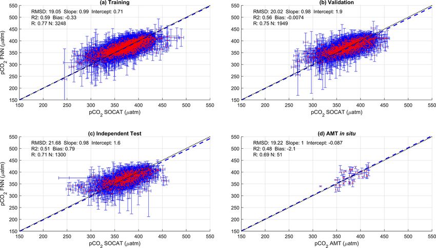
96                                            D. J. Ford et al.: Derivation of seawater pCO2 from net community production

Table 2. The input parameters of the neural network variants described in Sects. 2.3. and 2.6. xCO2 is the atmospheric mixing ratio of CO2 .

                             Neural network variant           Input parameters
                             SA-FNNNCP                        pCO2 (atm) , SST and NCP
                             SA-FNNNPP                        pCO2 (atm) , SST and NPP
                             SA-FNNCHLA                       pCO2 (atm) , SST and Chl a
                             SA-FNNNO-BIO-1                   pCO2 (atm) and SST
                             SA-FNNNO-BIO-2                   pCO2 (atm) , SST, salinity and mixed layer depth
                             W2020 (Watson et al., 2020a)     xCO2 (atm) , SST, salinity and mixed layer depth

the equatorial region was merged into one province. In each             output from the eight province FNNs was then combined,
province the available monthly pCO2 (sw) observations were              and weighted statistics, which account for both the satellite
matched to temporally and spatially coincident pCO2 (atm) ,             and in situ uncertainty, were used to assess the overall perfor-
MODIS-A, NCP and SST to provide training data for the                   mance of the FNN (as also used in Ford et al., 2021b). The
feed forward neural network (FNN). Observations in coastal              combined eight-FNN approach will hereafter be referred to
regions (< 200 m water depth) were removed from the analy-              as SA-FNN.
sis, due to the increased uncertainty in ocean colour observa-             The approach to training the FNNs was repeated replac-
tions in these areas (e.g. Lavender et al., 2004). Due to con-          ing NCP with Chl a or NPP sequentially (Table 2) to deter-
straints on the coverage of ocean colour data, no data were             mine if there was an improvement by using NCP. Chl a and
available in austral winter below ∼ 50◦ S.                              NPP estimates were log10 -transformed before input into the
   The coincident observations in each province were ran-               FNN, due to their respective uncertainties being determined
domly split into three datasets: (1) a training data set (50 %          in log10 space (Table 1). A baseline SA-FNN with no bio-
of the observations) used to train the FNNs; (2) a validation           logical parameters as input was trained using pCO2 (atm) and
data set (30 % of the observations) used to assess the perfor-          MODIS-A SST (SA-FNNNO-BIO-1 ; Table 2). A second SA-
mance of the FNN and to prevent the networks from overfit-              FNN with no biological parameters (SA-FNNNO-BIO-2 ; Ta-
ting; and (3) an independent test data set (20 % of the obser-          ble 2) was trained with the addition of sea surface salinity and
vations) to assess the final performance of the FNN, with ob-           mixed layer depth from the Copernicus Marine Environment
servations that are independent of the network training. The            Modelling Service (https://resources.marine.copernicus.eu/,
optimal split (ropt ) method of Amari et al. (1997) was used            last access: 20 August 2020) global ocean physics reanal-
to partition the input data into these three sets, as follows:          ysis product (GLORYS12V1). This parameter combination
                                                                        (pCO2 (atm) , SST, salinity and mixed layer depth) has recently
            1                                                           been included within a neural network scheme to estimate
ropt = 1 − √ ,                                                  (1)
            2m                                                          global fields of pCO2 (sw) (Watson et al., 2020b).
                                                                           Following these methods, a monthly mean time series of
where m is number of input parameters. For our three input              pCO2 (sw) was generated in the South Atlantic Ocean, ap-
parameters, an optimal split of 60 % training data to 40 %              plying the SA-FNN approach using NCP (SA-FNNNCP ),
validation data would occur, where we removed 10 % from                 NPP (SA-FNNNPP ), Chl a (SA-FNNCHLA ) or no biolog-
each data set to provide a further independent test data set. A         ical parameters (SA-FNNNO-BIO-1 and SA-FNNNO-BIO-2 ).
pre-training step was used to determine the optimum num-                The pCO2 (sw) fields were spatially averaged using a
ber of hidden neurons in the FNN (Benallal et al., 2017;                3 pixel × 3 pixel filter but were not averaged temporally as
Landschützer et al., 2013; Moussa et al., 2016) to provide              in previous studies (Landschützer et al., 2014, 2016) because
the best fit for the observations, whilst preventing overfitting        averaging temporally could mask features that occur within
(Demuth et al., 2008).                                                  single months of the year. The uncertainties in the input pa-
   The FNNs consist of one hidden layer with between 2                  rameters (Table 1) were propagated through the neural net-
and 30 nodes depending on the pre-training step and one                 work on a per-pixel basis and combined in quadrature with
output layer. The networks were trained using the optimum               the RMSD of the test data set to produce a combined uncer-
number of hidden neurons, in an iterative process until the             tainty budget for each pixel, assuming all sources of uncer-
root mean square difference (RMSD) remained unchanged                   tainty are independent and uncorrelated (BIPM, 2008; Tay-
for six iterations. The best-performing FNN, with the low-              lor, 1997).
est RMSD, was then used to estimate pCO2 (sw) . The uncer-
tainties in the input parameters were propagated through the            2.4    Atlantic Meridional Transect in situ data
FNN, using a Monte Carlo uncertainty propagation, where
1000 calculations were made perturbing the input parame-                To assess the accuracy of the SA-FNN, coincident in situ
ters, using random noise for their uncertainty (Table 1). The           measurements of NCP, NPP, Chl a, SST, pCO2 (atm) and

Biogeosciences, 19, 93–115, 2022                                                               https://doi.org/10.5194/bg-19-93-2022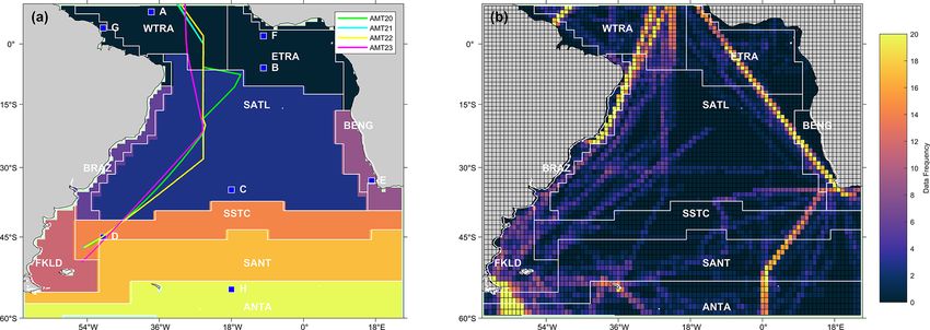
D. J. Ford et al.: Derivation of seawater pCO2 from net community production                                                  97

pCO2 (sw) , with uncertainties, were provided by Atlantic         three training datasets and on the Atlantic Meridional Tran-
Meridional Transects 20, 21, 22 and 23 in 2010, 2011, 2012        sect in situ data. The analysis was repeated sequentially re-
and 2013, respectively. All the Atlantic Meridional Transect      placing NCP with Chl a and NPP to determine if there was a
data described in this section can be obtained from the British   greater maximum reduction in RMSD using NCP. The analy-
Oceanographic Data Centre (https://www.bodc.ac.uk/, last          sis was also conducted allowing for a 10 % reduction in input
access: 11 April 2020). Chl a was computed following              parameter uncertainties to indicate the short-term reduction
the methods of Brewin et al. (2016), using underway con-          in pCO2 (sw) RMSD that could be achieved by reducing the
tinuous spectrophotometric measurements from AMT 22,              input parameter uncertainties.
and uncertainties were estimated as ∼ 0.06 log10 (mg m−3 )
(Ford et al., 2021b). 14 C-based NPP measurements were            2.6   Comparison of the SA-FNNNCP with the
made based on dawn-to-dusk simulated in situ incuba-                    SA-FNNNO-BIO , SA-FNNCHLA , SA-FNNNPP and
tions, following the methods given in Tilstone et al. (2017),           state-of-the-art data for the South Atlantic
at 56 stations with a per-station uncertainty. Uncertainties
ranged between 8 and 213 mg C m−2 d−1 and were on av-             The most comprehensive pCO2 (sw) fields to date are from
erage 53 mg C m−2 d−1 . NCP was estimated using in vitro          Watson et al. (2020a, b). The “standard method” pCO2 (sw)
changes in dissolved O2 , following the methods of Gist           fields within the Watson et al. (2020a, b) data were pro-
et al. (2009) and Tilstone et al. (2015) at 51 stations with      duced by extrapolating the in situ reanalysed SOCATv2019
a per-station uncertainty calculated. Uncertainties ranged        pCO2 (sw) observations using a self-organising-map feed for-
between 5 and 25 mmol O2 m−2 d−1 and were on average              ward neural network approach (Landschützer et al., 2016),
14 mmol O2 m−2 d−1 .                                              hereafter referred to as “W2020”. A time series was ex-
   Underway measurements of pCO2 (sw) and pCO2 (atm)              tracted from the W2020 data, coincident with SA-FNNNCP ,
were performed continuously, following the methods of Ki-         SA-FNNNPP , SA-FNNCHLA and the two SA-FNNNO-BIO
tidis et al. (2017). SST was continuously measured alongside      variants. For the six methods, a monthly climatology ref-
all observations (Sea-Bird SBE45), with a factory-calibrated      erenced to the year 2010 was computed, assuming an at-
uncertainty of ± 0.01 ◦ C. The mean of underway pCO2 (sw) ,       mospheric CO2 increase of 1.5 µatm yr−1 (Takahashi et al.,
pCO2 (atm) , SST and Chl a were taken ± 20 min around             2009; Zeng et al., 2014). The climatology should be insensi-
each station where NCP and NPP were measured. These               tive to the assumed rise in atmospheric CO2 due to the ref-
pCO2 (sw) observations (N ≈ 200) were removed from the            erence year being central to the time series. The standard de-
SOCATv2020 data set so that the Atlantic Meridional Tran-         viation of this climatology was also computed on a per-pixel
sect data remained independent from the training and valida-      basis.
tion datasets.                                                       The stations (Fig. 1) are representative of locations from
                                                                  previous literature that analysed the variability of in situ
2.5   Perturbation analysis                                       pCO2 (sw) in the South Atlantic Ocean. For each station, the
                                                                  monthly climatology of pCO2 (sw) , representing the average
Following the approach of Saba et al. (2011), a perturbation      seasonal cycle of pCO2 (sw) , and the standard deviation of the
analysis was conducted to evaluate the potential reduction        climatology, as an indication of the interannual variability,
in SA-FNN pCO2 (sw) RMSD that could be attributed to the          were extracted from the six approaches. The pCO2 (sw) value
input parameters. The analysis indicates the maximum re-          for each station was the statistical mean of the four nearest
duction in RMSD that could be achieved if uncertainties in        data points weighted by their respective proximity to the sta-
the input parameters were reduced to ∼ 0. Each of the input       tion coordinate. In situ pCO2 (sw) observations from the SO-
parameters – NCP, SST and pCO2 (atm) – can have three pos-        CATv2020 Flag E data set were also extracted for stations A
sible values for each in situ pCO2 (sw) observation (original     and B (Fig. 1a), and a climatology was generated. These ob-
value, original ± uncertainty; Table 1), enabling 27 pertur-      servations represent data from the Prediction and Research
bations of the input data as input to the SA-FNN. For each        Moored Array in the Atlantic (PIRATA) buoys at these loca-
in situ pCO2 (sw) observation, the 27 perturbations of SA-        tions (Bourlès et al., 2008).
FNN pCO2 (sw) were examined, and the perturbation that pro-          The station climatologies for the SA-FNNNO-BIO-1 ,
duced the lowest RMSD and bias combination was selected.          SA-FNNNO-BIO-2 , W2020, SA-FNNCHLA and SA-FNNNPP
The RMSD and bias were calculated between all the in situ         were compared to the SA-FNNNCP , by testing for signifi-
pCO2 (sw) and the selected perturbations. The percentage dif-     cant differences in the seasonal cycle and annual pCO2 (sw)
ference between this RMSD and the original RMSD when              (offset). The seasonal cycles (seasonality) were compared
training the SA-FNN was calculated to indicate the maxi-          using a non-parametric Spearman correlation and deemed
mum achievable reduction. This approach was conducted for         statistically different where the correlation was not signifi-
two scenarios: (1) uncertainty in individual input parame-        cant (α < 0.05). A non-parametric Kruskal–Wallis test was
ters (NCP, SST and pCO2 (atm) ) and (2) uncertainty in all in-    used to test for significant (α < 0.05) differences in the an-
put parameters together. The approach was conducted on all        nual pCO2 (sw) , indicating an offset between the two tested

https://doi.org/10.5194/bg-19-93-2022                                                        Biogeosciences, 19, 93–115, 2022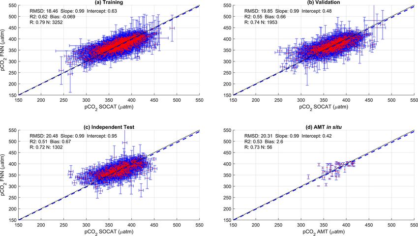
98 D. J. Ford et al.: Derivation of seawater pCO2 from net community production
climatologies. The Southern Ocean station (station H) was and a precision (bias) of 0.87 µatm, which was determined
excluded from the statistical analysis due to missing data in with the independent test data (N = 1300). Training the SA-
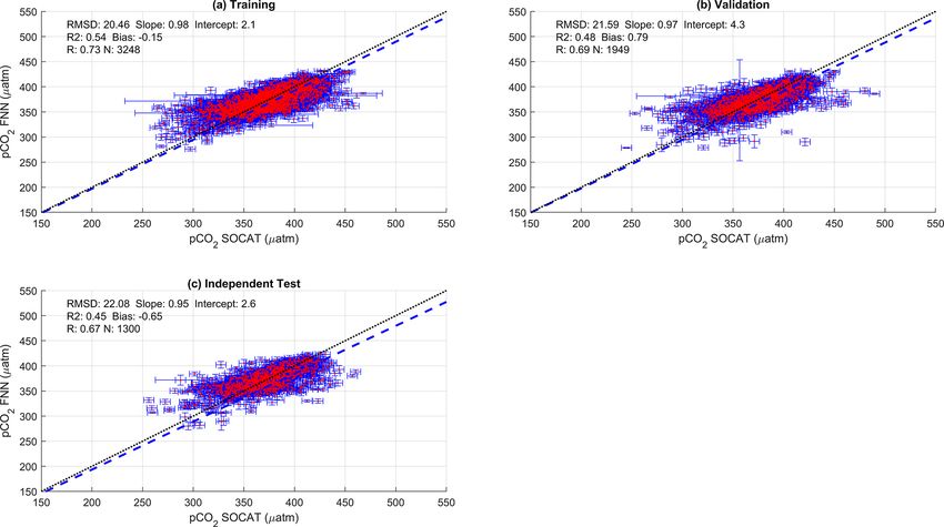
the SA-FNN. FNN using Chl a or NPP instead of NCP resulted in a similar
performance (Appendix A Figs. A1 and A2). The RMSD for
2.7 Estimation of the bulk CO2 flux the independent test data was within ∼ 1.5 µatm for Chl a
(19.88 µatm), NPP (20.48 µatm) and NCP (21.68 µatm), and
The flux of CO2 (F ) between the atmosphere and ocean (air– bias was near zero.
sea) can be expressed in a bulk parameterisation as The reduction in pCO2 (sw) RMSD that could be achieved
if input parameter uncertainties were reduced to ∼ 0 was as-
F = k(αw pCO2 (sw) − αs pCO2 (atm) ), (2) sessed using the perturbation analysis (Table 3, Appendix A
Table A1). This showed that a reduction in pCO2 (sw) RMSD
where k is the gas transfer velocity, and αw and αs are the
of 36 % was achieved by eliminating satellite NCP uncertain-
solubility of CO2 at the base and top of the mass bound-
ties, 34 % was achieved by eliminating satellite NPP uncer-
ary layer at the sea surface, respectively (Woolf et al., 2016).
tainties and 19 % was achieved by eliminating satellite Chl a
k was estimated from ERA5 monthly reanalysis wind speed
uncertainties. The bias remained near zero for all parame-
(downloaded from the Copernicus Climate Data Store; https:
ters, indicating good precision of the SA-FNN approach (not
//cds.climate.copernicus.eu/, last access: 12 March 2020) fol-
shown). Applying the Atlantic Meridional Transect in situ
lowing the parameterisation of Nightingale et al. (2000). The
data as input to the SA-FNN and using the perturbation anal-
parameter αw was estimated as a function of SST and sea sur-
ysis, a decrease in pCO2 (sw) RMSD of 25 % for NCP, 13 %
face salinity (Weiss, 1974) using the monthly Optimum Inter-
for NPP and 7 % for Chl a was observed.
polated SST (Reynolds et al., 2002) and sea surface salinity
The reduction in pCO2 (sw) RMSD from reducing input
from the Copernicus Marine Environment Modelling Service
parameter uncertainties by 10 % was also assessed through
global ocean physics reanalysis product (GLORYS12V1).
the perturbation analysis (Table 4). This indicated a decrease
The αs parameter was estimated using the same temperature
in pCO2 (sw) RMSD of 8 % for NCP, 5 % for NPP and 2 %
and salinity datasets but included a gradient from the base to
for Chl a, again indicating that improving NCP uncertainties
the top of mass boundary layer of −0.17 K (Donlon et al.,
has the largest impact on improving the estimated pCO2 (sw)
1999) and +0.1 salinity units (Woolf et al., 2016). pCO2 (atm)
fields.
was estimated using the dry mixing ratio of CO2 from the
NOAA-ESRL marine boundary layer reference, Optimum
Interpolated SST (Reynolds et al., 2002) applying a cool 3.2 Comparison between SA-FNNNCP and other
skin bias (0.17 K; Donlon et al., 1999) and sea level pres- methods
sure following Dickson et al. (2007). Spatially and tempo-
rally complete pCO2 (sw) fields, which are representative of
The monthly climatologies of pCO2 (sw) generated us-
pCO2 (sw) at the base of the mass boundary layer, were ex-
ing the SA-FNNNCP and referenced to the year 2010
tracted from the SA-FNNNCP , SA-FNNNPP , SA-FNNCHLA ,
showed differences with two published climatologies, es-
SA-FNNNO-BIO-1 , SA-FNNNO-BIO-2 and W2020.
pecially in the equatorial region (Appendix B). The
The monthly CO2 flux was calculated using the open-
monthly climatology for eight stations (Fig. 1) was ex-
source FluxEngine toolbox (Holding et al., 2019; Shutler
tracted from the SA-FNNNCP , SA-FNNNPP , SA-FNNCHLA ,
et al., 2016) between 2003 and 2018 for the six pCO2 (sw)
SA-FNNNO-BIO-1 , SA-FNNNO-BIO-2 and the W2020 to as-
inputs, using the “rapid transport” approximation (described
sess differences between the pCO2 (sw) estimates (Fig. 3).
in Woolf et al., 2016). The net annual flux was determined for
The SA-FNNNCP and SA-FNNNO-BIO-1 showed significant
the South Atlantic Ocean (10◦ N–44◦ S, 25◦ E–70◦ W) using
divergence in the equatorial Atlantic (Figs. 3b, f, g and 4).
the “fe_calc_budgets.py” utility within FluxEngine with the
At the eastern equatorial station, the interannual variability
supplied area and land percentage masks. The mean net an-
in pCO2 (sw) from the SA-FNNNCP was high, and a min-
nual flux was calculated as the mean of the 15-year net an-
imum occurred between January and April, which gradu-
nual fluxes. Positive net fluxes indicate a net source to the
ally increased to a maximum in September and October
atmosphere, and negative net fluxes represent a sink.
(Fig. 3b). The SA-FNNNO-BIO-1 showed no seasonality in
the pCO2 (sw) and was consistently below the SA-FNNNCP
3 Results pCO2 (sw) . The Gulf of Guinea station showed a similar vari-
ability in the SA-FNNNCP pCO2 (sw) except that the max-
3.1 SA-FNN performance and perturbation analysis ima was lower at this station (Fig. 3f). The SA-FNNNO-BIO-1
indicated pCO2 (sw) below the SA-FNNNCP throughout the
The performance of the SA-FNN trained using pCO2 (atm) , year. The greatest divergence occurred near the Amazon
SST and NCP for the three training datasets is given in Fig. 2. Plume (Fig. 3g) where SA-FNNNCP pCO2 (sw) was below or
The SA-FNNNCP had an accuracy (RMSD) of 21.68 µatm at pCO2 (atm) for all months and there was a large interan-
Biogeosciences, 19, 93–115, 2022 https://doi.org/10.5194/bg-19-93-2022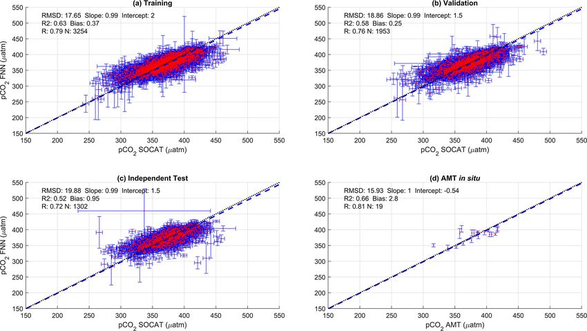
D. J. Ford et al.: Derivation of seawater pCO2 from net community production                                                                 99

Figure 2. Scatter plots showing the combined performance of the eight feed forward neural networks trained using NCP for each biogeochem-
ical province (Fig. 1) using four separate training and validation datasets: (a) training, (b) validation, (c) independent test and (d) Atlantic
Meridional Transect (AMT) in situ. The data points are highlighted in red to distinguish them from the error bars in blue. The blue dashed
line is the type II regression, and the black dashed line is the 1 : 1 line. Horizontal error bars indicate the uncertainty of the SOCATv2020
pCO2 (sw) . Vertical error bars indicate the uncertainty attributed to the input parameter uncertainty propagated through the feed forward
neural networks. The statistics within each plot are the root mean square difference (RMSD), slope and intercept of the type II regression,
coefficient of determination (R 2 ), Pearson correlation coefficient (R), bias and number of samples (N ).

Table 3. The percentage reduction in pCO2 (sw) RMSD by reducing NCP, NPP and Chl a uncertainties to ∼ 0 as described in Sect. 2.5. The
full results can be found in Appendix Table A1.

                          Parameter     Training [%]    Validation [%]     Independent test [%]     AMT in situ [%]
                          NCP                     32                 40                       36                  25
                          NPP                     31                 37                       36                  13
                          Chl a                   17                 21                       20                   7

nual variability in pCO2 (sw) . The SA-FNNNO-BIO-1 displayed              and Amazon Plume. In south Benguela (Figs. 3e and 4),
higher pCO2 (sw) and a lower interannual variability (Fig. 3g).           SA-FNNNCP had pCO2 (sw) maxima in austral summer,
   The SA-FNNNCP and SA-FNNNO-BIO-1 showed no signif-                     whereas the SA-FNNCHL maximum occurs in austral winter.
icant difference in the seasonal patterns of pCO2 (sw) at sta-            In the Amazon Plume there was significant offset between
tions south of 20◦ S (Figs. 3c–e and 4). There was, however,              the two methods, and the SA-FNNCHL resulted in lower
a significant offset at some stations where the SA-FNNNCP                 pCO2 (sw) compared to the SA-FNNNCP (Figs. 3g and 4).
generally exhibited lower pCO2 (sw) in austral summer and                 The SA-FNNNCP and SA-FNNNPP had a significant offset
a higher interannual variation. The SA-FNNNCP was signif-                 at the eastern equatorial station (Figs. 3c and 4), where the
icantly different to W2020 and SA-FNNNO-BIO-2 at similar                  SA-FNNNPP indicated lower pCO2 (sw) . For the other sta-
stations to those at which SA-FNNNO-BIO-1 was different                   tions, no significant differences were observed.
(Figs. 3 and 4).
   The SA-FNNNCP and SA-FNNCHLA showed significant
differences in pCO2 (sw) values in the south Benguela

https://doi.org/10.5194/bg-19-93-2022                                                                   Biogeosciences, 19, 93–115, 2022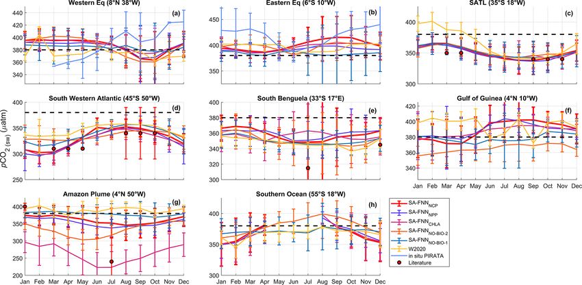
100 D. J. Ford et al.: Derivation of seawater pCO2 from net community production
Table 4. The percentage reduction in pCO2 (sw) RMSD by reducing NCP, net primary production and chlorophyll a uncertainties by 10 % as
described in Sect. 2.5.
Parameter Training [%] Validation [%] Independent test [%] AMT in situ [%]
NCP 7 8 8 3
NPP 5 6 5 1.5
Chl a 2 2 2 0.5
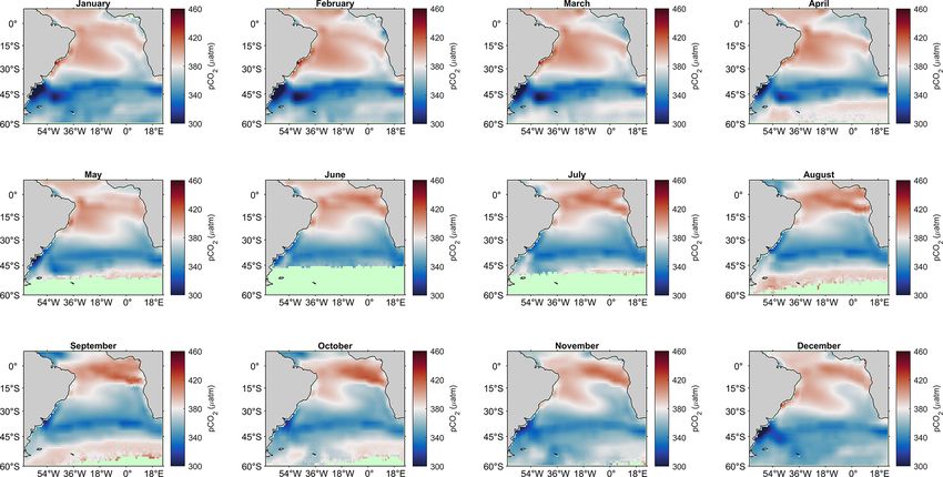
Figure 3. Monthly climatologies of pCO2 (sw) referenced to the year 2010 for the eight stations marked in Fig. 1 from the SA-FNNNCP ,
SA-FNNNPP , SA-FNNCHLA , SA-FNNNO-BIO-1 , SA-FNNNO-BIO-2 and W2020 (Watson et al., 2020b). Light blue lines in Fig. 3a and b
indicate the in situ pCO2 (sw) observations from PIRATA buoys. The atmospheric CO2 increase was set as 1.5 µatm yr−1 . Black dashed
line indicates the atmospheric pCO2 (∼ 380 µatm). Error bars indicate the 2 standard deviations of the climatology (∼ 95 % interval), where
larger error bars indicate a larger interannual variability. Red circles indicate the literature values of pCO2 (sw) described in Sect. 4.2. Note
the different y-axis limits in each plot.
4 Discussion ing pCO2 (sw) could be achieved if NCP data uncertainties
were reduced (Table 3). A similar improvement could be ob-
4.1 Assessment of biological parameters to estimate tained if the NPP uncertainties were reduced (Table 3). Ford
pCO2 (sw) et al. (2021b) showed that up to 40 % of the uncertainty in
satellite NCP is attributed to the uncertainty in satellite NPP,
which is an input to the NCP approach. This suggests that
In this paper, the differences in estimating pCO2 (sw) us-
improvements in estimating NPP from satellite data will lead
ing FNNs with satellite-derived NCP, NPP or Chl a
to a further improvement in estimating pCO2 (sw) from NCP.
were assessed. The SA-FNNNCP had an overall accuracy
These improvements could be achieved through better esti-
(21.68 µatm; Fig. 2) that is consistent with other approaches
mates of the water column light field (e.g. Sathyendranath
that have been developed for the Atlantic (22.83 µatm; Land-
et al., 2020) and the vertical variability of input parameters
schützer et al., 2013) and slightly lower than the published
or assignment of photosynthetic parameters (e.g. Kulk et al.,
global result of 25.95 µatm (Landschützer et al., 2014).
2020), for example. For a discussion on improving satellite
Training the SA-FNN using Chl a or NPP showed compa-
NPP estimates we refer the reader to Lee et al. (2015).
rable broadscale accuracy to NCP. When the uncertainties in
To uncouple the Chl a, NPP, and NCP estimates and their
the input parameters were investigated, however, differences
uncertainties, the perturbation analysis was also conducted
in the estimates of pCO2 (sw) were apparent. The perturbation
on Atlantic Meridional Transect in situ observations. This
analysis indicated that up to a 36 % improvement in estimat-
Biogeosciences, 19, 93–115, 2022 https://doi.org/10.5194/bg-19-93-2022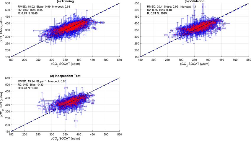
D. J. Ford et al.: Derivation of seawater pCO2 from net community production                                                        101

Figure 4. Statistical comparison of the SA-FNNNCP with the W2020, SA-FNNNO-BIO-1 , SA-FNNNO-BIO-2 , SA-FNNCHLA and
SA-FNNNPP climatologies, where yellow blocks indicate a significant difference (α = 0.05). Seasonality indicates a difference in the sea-
sonal cycle, and offset indicates a difference between the mean pCO2 (sw) of the climatologies.

showed that reducing in situ NCP uncertainties provided the            gories: (a) in vitro incubations of samples under light/dark
greatest reduction in pCO2 (sw) RMSD, which was 3 times                treatments (Gist et al., 2009) and (b) in situ observations
the reduction achievable using Chl a (Tables 3 and 4). This            of oxygen-to-argon (O2 /Ar) ratios (Kaiser et al., 2005) or
indicates that the optimal predictive power of Chl a to esti-          the observed isotopic signature of oxygen (Kroopnick, 1980;
mate pCO2 (sw) has been reached and that to achieve further            Luz and Barkan, 2000). All of these methods are subject to,
improvements in estimates of pCO2 (sw) and reduction in its            but do not account for, the photochemical sink, which may
associated uncertainty requires the use of NCP.                        lead to underestimation of in vitro NCP by up to 22 % (Ki-
   A reduction of input uncertainties to ∼ 0 is near impos-            tidis et al., 2014). Independent ground measurements that
sible, but a reduction by 10 % could be feasible (e.g. NCP             use accepted protocols for the in vitro method are currently
uncertainty reduced from 45 to 40.5 mmol O2 m−2 d−1 ; Ta-              made on the Atlantic Meridional Transect; however, a com-
ble 1). A perturbation analysis conducted for this showed              munity consensus should consider a consistent methodology
similar results, with NCP producing the greatest reduction in          for NCP. Increasing the number of such observations for the
pCO2 (sw) RMSD of 8 % compared to 2 % for Chl a (Table 4).             purpose of algorithm development would further constrain
Thus, reducing NCP uncertainties will provide a greater im-            the NCP but also provide observations across the lifetime of
provement in pCO2 (sw) compared to reducing the uncertain-             newly launched satellites. The uncertainties on each in vitro
ties in Chl a.                                                         measurement are assessed through replicate bottles which
   These improvements in estimating NCP could be achieved              could be used to calculate a full uncertainty budget for each
through many components. Ford et al. (2021b) showed that               NCP measurement when combined with analytical uncer-
40 % of satellite NCP uncertainties were attributed to in              tainties.
situ NCP uncertainties. The in situ bottle incubation mea-                Serret et al. (2015) indicated that NCP is controlled by
surements could be improved using the principles of Fidu-              both the heterogeneity in NPP and respiration. The satellite
cial Reference Measurements (FRM; Banks et al., 2020),                 NCP algorithm applied in this study accounts for some of
which are traceable to metrology standards, referenced to              the heterogeneity in respiration, through an empirical SST-
inter-comparison exercises, with a full uncertainty budget.            to-NCP relationship (Tilstone et al., 2015). Quantifying the
This becomes complicated, however, when considering the                variability in respiration could further improve NCP esti-
number of different methods to measure NCP and the large               mates when coupled with NPP rates from satellite observa-
divergence between them (Robinson et al., 2009). A re-                 tions.
view of these methods has already been conducted (Duarte
et al., 2013; Ducklow and Doney, 2013; Williams et al.,
2013). The methods broadly fall into the following cate-

https://doi.org/10.5194/bg-19-93-2022                                                              Biogeosciences, 19, 93–115, 2022
102                                         D. J. Ford et al.: Derivation of seawater pCO2 from net community production

4.2   Accuracy of SA-FNNNCP pCO2 (sw) at seasonal and              ability in SA-FNNNCP pCO2 (sw) clearly shows the influence
      interannual scales                                           of the equatorial upwelling at these stations, with latitudinal
                                                                   gradients in pCO2 (sw) during the upwelling period (Lefèvre
The seasonal and interannual variability of pCO2 (sw) es-          et al., 2016), but struggles to identify elevated pCO2 (sw) be-
timated using the SA-FNNNCP was compared with the                  tween December and April shown by the PIRATA buoy ob-
SA-FNNNO-BIO , W2020 (Watson et al., 2020b), SA-FNNCHL             servations (Fig. 3b). By contrast, the SA-FNNNO-BIO-1 in-
and SA-FNNNPP at eight stations. The stations (Fig. 1) rep-        dicated little influence from the equatorial upwelling and a
resent locations of previous studies into in situ pCO2 (sw)        depressed pCO2 (sw) during the upwelling season.
variability, allowing comparisons with literature values.             The two methods converge on the seasonal cycle at the re-
Significant differences between the SA-FNNNCP and                  maining stations, although significant offsets in the mean an-
SA-FNNNO-BIO were observed at four stations (Fig. 4), es-          nual pCO2 (sw) remain. The station at 35◦ S, 18◦ W (Fig. 3c)
pecially in the equatorial Atlantic.                               has consistently been implied as a sink for CO2 . Lencina-
   At 8◦ N, 38◦ W (Fig. 3a), Lefèvre et al. (2020) reported        Avila et al. (2016) showed the region to have 340 µatm
pCO2 (sw) to be stable at ∼ 400 µatm, between June and Au-         pCO2 (sw) and to be a sink for CO2 between October and
gust 2013, and to decrease in September to ∼ 360 µatm,             December. Similarly, Kitidis et al. (2017) implied that the
which is attributed to the Amazon Plume propagating into           region is a sink for CO2 during March to April. The re-
the western equatorial Atlantic (Coles et al., 2013). Bruto        gion has depressed pCO2 (sw) due to high biological activ-
et al. (2017) indicated, however, that elevated pCO2 (sw) at       ity that originates from the Patagonian Shelf and the South
∼ 430 µatm was observed in September for 2008 to 2011.             Subtropical Convergence Zone. The station at 45◦ S, 50◦ W
The error bars on the PIRATA buoy pCO2 (sw) observations           (Fig. 3d) has also been implied as a strong but highly variable
(Fig. 3a) clearly highlight the differences between Lefèvre        sink, where pCO2 (sw) can be between ∼ 280 and ∼ 380 µatm
et al. (2020) and Bruto et al. (2017), but there are less than     during austral spring and is constant at ∼ 310 µatm during
4 years of monthly observations available, which do not re-        austral autumn (Kitidis et al., 2017). The SA-FNNNCP and
solve the full seasonal cycle. For the station in the Ama-         SA-FNNNO-BIO-1 methods reproduced the seasonal variabil-
zon Plume at 4◦ N, 50◦ W (Fig. 3g), where the effects of the       ity in the pCO2 (sw) at these two stations accurately, but only
plume extend northwest towards the Caribbean (Coles et al.,        the SA-FNNNCP captures the magnitude of the depressed
2013; Varona et al., 2019), Lefèvre et al. (2017) indicated that   pCO2 (sw) at 45◦ S.
this region acts as a sink for CO2 (pCO2 (sw) < pCO2 (atm) ),         Within the southern Benguela upwelling system,
especially between May and July, coincident with maximum           pCO2 (sw) at station 33◦ S, 17◦ E (Fig. 3e) is influenced by
discharge from the Amazon River (Dai and Trenberth, 2002).         gradients in the seasonal upwelling (Hutchings et al., 2009).
Valerio et al. (2021) indicated pCO2 (sw) varied at and below      Santana-Casiano et al. (2009) showed that pCO2 (sw) varies
pCO2 (atm) at 4◦ N, 50◦ W, consistent with the SA-FNNNCP .         from ∼ 310 µatm in July to ∼ 340 µatm in December and that
The interannual variability of pCO2 (sw) has been shown to be      the region is a CO2 sink through the year. González-Dávila
high in this region in all months (Lefèvre et al., 2017). The      et al. (2009) suggested, however, that this CO2 sink is highly
SA-FNNNCP provided a better representation of the seasonal         variable during upwelling events and that recently upwelled
and interannual variability induced by the Amazon River dis-       waters act as a source (pCO2 (sw) > pCO2 (atm) ) of CO2
charge and associated plume at these two stations compared         to the atmosphere (Gregor and Monteiro, 2013). Arnone
to the SA-FNNNO-BIO , although differences were small at           et al. (2017) indicated elevated pCO2 (sw) during austral
8◦ N, 38◦ W.                                                       spring and autumn at the station, with a ∼ 40 µatm seasonal
   The station in the eastern tropical Atlantic at 6◦ S, 10◦ W     cycle amplitude. The SA-FNNNCP and SA-FNNNO-BIO-1
(Fig. 3b) is under the influence of the equatorial upwelling       were able to reproduce the seasonal cycle, although the
(Lefèvre et al., 2008), which is associated with the upwelling     SA-FNNNCP correctly represented the seasonal magnitude
of CO2 -rich waters between June and September. Lefèvre            in pCO2 (sw) as reported by Santana-Casiano et al. (2009)
et al. (2008) indicated that peak pCO2 (sw) of ∼ 440 µatm was      and Arnone et al. (2017).
observed in September and remained stable until December,             In summary, for these stations, the SA-FNNNCP bet-
before decreasing to a minima of ∼ 360 µatm in May (Parard         ter represents the seasonality and the interannual variabil-
et al., 2010). Lefèvre et al. (2016) showed, however, that the     ity of pCO2 (sw) in the South Atlantic Ocean compared to
influence of the equatorial upwelling does not reach the buoy      the SA-FNNNO-BIO-1 , especially in the equatorial Atlantic.
in all years, and in some years lower pCO2 (sw) is observed.       The SA-FNNNO-BIO-2 also displayed significant differences
The PIRATA buoy observations (Fig. 3b) clearly show this           compared to SA-FNNNCP , indicating that the variability in
seasonality but also highlight the interannual variability in in   pCO2 (sw) has a strong biological contribution which is not
situ pCO2 (sw) . Further north at 4◦ N, 10◦ W (Fig. 3f), Koffi     fully represented and explained by the additional physi-
et al. (2010) suggested that this region follows a similar sea-    cal parameters included in the FNN. The SA-FNNNO-BIO-2
sonal cycle as the station at 6◦ S, 10◦ W but that pCO2 (sw)       and W2020 both displayed significant differences compared
is ∼ 30 µatm lower (Koffi et al., 2016). The interannual vari-     to the SA-FNNNCP at specific stations (Fig. 4). There are

Biogeosciences, 19, 93–115, 2022                                                        https://doi.org/10.5194/bg-19-93-2022
D. J. Ford et al.: Derivation of seawater pCO2 from net community production 103 methodological differences between these approaches, how- with in situ pCO2 (sw) observations at 4◦ N, 50◦ W, where ever. The SA-FNN method uses only in situ pCO2 (sw) ob- pCO2 (sw) varied at or below pCO2 (atm) (Valerio et al., 2021). servations from the South Atlantic Ocean to train the FNNs. Though the differences between the SA-FNNNCP and The W2020 uses global in situ pCO2 (sw) observations to train SA-FNNCHLA may appear small, the Amazon Plume and FNNs for 16 provinces with similar seasonal cycles (Land- Benguela Upwelling have a higher intensity in the CO2 schützer et al., 2014; Watson et al., 2020b). The W2020 will flux per unit area compared to the open ocean, illustrat- therefore be weighted to pCO2 (sw) variability in regions of ing a disproportionate contribution to the overall global relatively abundant in situ observations (i.e. Northern Hemi- CO2 sink than their small areal coverage implies (Laru- sphere) and may not be fully representative of the South At- elle et al., 2014). The differences in the pCO2 (sw) estimates lantic Ocean. This would explain the SA-FNNNO-BIO-2 and result in a 22 Tg C yr−1 alteration in the annual CO2 flux W2020 differences, when driven using the same input vari- for the South Atlantic Ocean (SA-FNNNCP = +14 Tg C yr−1 ; ables. SA-FNNCHLA = −9 Tg C yr−1 ; Fig. 5f). This unequivocally Comparing the SA-FNNNCP and SA-FNNCHLA there were reinforces the use of NCP to improve basin-scale estimates two significant differences (Fig. 4). A difference in the sea- of pCO2 (sw) , especially in regions where Chl a, NPP and sonal cycle in the southern Benguela (Fig. 3e) was ob- NCP become disconnected. served. Santana-Casiano et al. (2009) showed that the min- Recent assessments of the strength of the global oceanic ima pCO2 (sw) in July and maxima in December, consis- CO2 sink have been made using pCO2 (sw) fields estimated tent with the SA-FNNNCP and SA-FNNNPP , whereas the using no biological parameters as input (Watson et al., SA-FNNCHL estimated the opposite scenario. Lamont et al. 2020b). Our results indicate that the SA-FNNNCP more ac- (2014) reported Chl a concentrations to remain consis- curately represented the pCO2 (sw) variability in the South tent in May and October, but NPP rates were significantly Atlantic Ocean compared to the SA-FNNNO-BIO-2 , which in- higher in October, associated with increased surface PAR cluded additional physical parameters. Estimating the South and enhanced upwelling. The disconnect between Chl a and Atlantic Ocean net CO2 flux with the SA-FNNNCP pCO2 (sw) NPP can also be observed in the satellite observations (Ap- produced a 14 Tg C yr−1 source compared to a 10 Tg C yr−1 pendix C Fig. C1), limiting the ability of Chl a to esti- sink indicated by the SA-FNNNO-BIO-2 (Fig. 5f). The in- mate pCO2 (sw) , which is highlighted by the failure of the cremental inclusion of parameters to account for the bio- SA-FNNCHLA to identify the seasonal pCO2 (sw) cycle. logical signal starting with Chl a (−9 Tg C yr−1 ), then NPP A Chl a-to-NPP disconnect has also been reported in the (−7 Tg C yr−1 ) and then NCP (+14 Tg C yr−1 ) switched the Amazon Plume (Smith and Demaster, 1996), where Chl a South Atlantic Ocean from a CO2 sink to a source, which concentrations can be similar but NPP rates significantly is driven by differences in the pCO2 (sw) estimates in regions different due to light limitation caused by suspended sed- that are biologically controlled. This 21 Tg C yr−1 difference iments. A significant offset between the SA-FNNNCP and between the SA-FNNNCP and SA-FNNNPP is due to addi- SA-FNNCHLA was observed in this region (Figs. 3g and 4). tional outgassing in the equatorial Atlantic provinces of the Lefèvre et al. (2017) reported pCO2 (sw) values ranging from WTRA and ETRA (Figs. 1a and 5f). Compared to the in 400 ± ∼ 10 µatm in January to ∼ 240 ± ∼ 70 µatm in May. situ pCO2 (sw) observations at the equatorial stations (Fig. 3a Although, the SA-FNNNCP January estimates are consistent, and b), it is likely that the outgassing is still underestimated the May estimates are higher than these in situ measure- by the SA-FNNNCP but does improve these estimates within ments. These observations were made further north (6◦ N) the upwelling season (June–September). where the turbidity within the plume has decreased suffi- The W2020 identified the South Atlantic Ocean as a ciently for irradiance to elevate NPP rates (Smith and De- source for CO2 of 15 Tg C yr−1 , which is consistent with the master, 1996), which decrease pCO2 (sw) . Chl a remains rel- SA-FNNNCP (Fig. 5f). The SA-FNNNCP , however, indicated atively consistent across the plume (not shown), suggest- the equatorial Atlantic (10◦ N to 20◦ S) as a 20 Tg C yr−1 ing a disconnect between Chl a and NPP at 4◦ N, 50◦ W, stronger source and south of 20◦ S (20◦ S to 44◦ S) as a which would lead to lower pCO2 (sw) estimates by the 20 Tg C yr−1 stronger sink. These differences indicate that SA-FNNCHLA , where NPP rates are low due to light limi- biologically induced variability in pCO2 (sw) would not be tation (Chen et al., 2012; Smith and Demaster, 1996). Respi- captured by the W2020 and could reduce the variability in ration would be elevated from the decomposition of riverine the global ocean CO2 sink. A further SA-FNN trained with organic material reducing NCP further (Cooley et al., 2007; pCO2 (atm) , SST, salinity, mixed layer depth and NCP indi- Jiang et al., 2019; Lefèvre et al., 2017). It is noted that the cated a similar CO2 source of 12 Tg C yr−1 (data not shown) Amazon Plume is a dynamic region with transient, localised as the SA-FNNNCP for the South Atlantic Ocean, highlight- biological and pCO2 (sw) features (Cooley et al., 2007; Ibán- ing that additional physical parameters cannot fully account hez et al., 2015; Lefèvre et al., 2017; Valerio et al., 2021) that for the biological contribution to the variability in pCO2 (sw) . may be masked by the coarse resolution of estimates avail- This further confirms the importance of using NCP within able using satellite data. The SA-FNNNCP , however, agreed estimates of the global ocean CO2 sink. https://doi.org/10.5194/bg-19-93-2022 Biogeosciences, 19, 93–115, 2022
104 D. J. Ford et al.: Derivation of seawater pCO2 from net community production
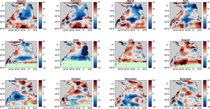
Figure 5. Long-term average annual mean CO2 flux for the South Atlantic Ocean, using pCO2 (sw) estimates from (a) SA-FNNNCP ,
(b) W2020 (Watson, et al., 2020a), (c) SA-FNNNO-BIO-2 , (d) SA-FNNCHLA and (e) SA-FNNNPP . (f) Bar chart displaying the mean annual
CO2 flux for different regions of the South Atlantic Ocean including 10◦ N to 44◦ S (whole South Atlantic Ocean), 10◦ N to 20◦ S, and 20 to
44◦ S, alongside the WTRA and ETRA biogeochemical provinces (Fig. 1a).
5 Conclusions equatorial Atlantic, in the upwelling region, a significant dif-
ference between the NCP and NPP approaches occurred. Sig-
In this paper, we compare neural network models of nificant differences between the NCP and Chl a approaches
pCO2 (sw) parameterised separately using either satellite were also observed in the Benguela upwelling and Amazon
Chl a, NPP or NCP as biological proxies to estimate com- Plume, where pCO2 (sw) from Chl a suggested that photosyn-
plete fields of pCO2 (sw) . The results suggest that using NCP thetic rates were not solely controlled by Chl a. Using NCP
improved the estimation of pCO2 (sw) . The differences be- to estimate pCO2 (sw) the South Atlantic Ocean was charac-
tween satellite Chl a, NPP or NCP were initially small, but terised as a net source of CO2 , whereas methods that only
the use of a perturbation analysis to assess the uncertainties include physical controls have indicated the region to be a
in these parameters showed that NCP has a greater poten- small sink for CO2 . Sequentially using Chl a to estimate
tial uncertainty reduction of up to ∼ 36 % of the RMSD, pCO2 (sw) and then NPP incrementally reduced the South At-
compared to a ∼ 19 % for Chl a. These results were veri- lantic CO2 sink, and finally using NCP the area switched to
fied using in situ observations from the Atlantic Meridional being a source of CO2 . These results indicate that in regions
Transect, which resulted in a 25 % improvement in pCO2 (sw) where biological activity is important in controlling the vari-
RMSD when the in situ NCP uncertainties were reduced to ability in pCO2 (sw) , the use of NCP, which is available from
∼ 0, compared to 7 % for Chl a and 13 % for NPP. satellite data, is important for quantifying the ocean carbon
Monthly climatological estimates of pCO2 (sw) at eight sta- pump and for providing data in areas that are sparsely cov-
tions in the South Atlantic Ocean, calculated using satel- ered by observations such as the Southern Ocean.
lite NCP, were compared with the NPP and the Chl a ap-
proaches and two neural networks that do not use biolog-
ical parameters. The NCP approach significantly improved
on both approaches with no biological parameters at four
stations in reconstructing the seasonal and interannual vari-
ability, compared to in situ pCO2 (sw) observations. At the
remaining four stations, differences were also observed, al-
though these were not statistically significant. In the eastern
Biogeosciences, 19, 93–115, 2022 https://doi.org/10.5194/bg-19-93-2022D. J. Ford et al.: Derivation of seawater pCO2 from net community production 105
Appendix A: Feed forward neural network training and
perturbation analysis
Table A1. The percentage reduction in root mean square difference (RMSD) attributable to the uncertainties in the input parameter for each
training and validation data set determined from a perturbation analysis as described in Sect. 2.5.
Parameter Training [%] Validation [%] Independent test [%] AMT in situ [%]
NCP ALL 33 42 38 28
SST 10 12 10 0.5
Net community production 32 40 36 25
pCO2 (atm) 6 7 6 9
Net primary production ALL 34 40 40 17
SST 9 10 10 0.4
Net primary production 31 37 36 13
pCO2 (atm) 6 6 6 9
Chlorophyll a ALL 22 26 25 29
SST 9 10 9 0.4
Chlorophyll a 17 21 20 7
pCO2 (atm) 8 9 9 16
Figure A1. Scatter plots showing the combined performance of the eight feed forward neural networks trained using chlorophyll a for four
separate training and validation datasets: (a) training, (b) validation, (c) independent test and (d) Atlantic Meridional Transect (AMT) in
situ. The blue dashed line is the type II regression, and the black dashed line is the 1 : 1 line. Horizontal error bars indicate the uncertainty of
the SOCATv2020 pCO2 (sw) . Vertical error bars indicate the uncertainty attributed to the input parameter uncertainty propagated through the
feed forward neural networks. The statistics within each plot are the root mean square difference (RMSD), slope and intercept of the type II
regression, coefficient of determination (R 2 ), Pearson correlation coefficient (R), bias and number of samples (N).
https://doi.org/10.5194/bg-19-93-2022 Biogeosciences, 19, 93–115, 2022You can also read