A high-resolution monitoring approach of canopy urban heat island using a random forest model and multi-platform observations
←
→
Page content transcription
If your browser does not render page correctly, please read the page content below
Atmos. Meas. Tech., 15, 735–756, 2022
https://doi.org/10.5194/amt-15-735-2022
© Author(s) 2022. This work is distributed under
the Creative Commons Attribution 4.0 License.

A high-resolution monitoring approach of canopy
urban heat island using a random forest model and
multi-platform observations
Shihan Chen1,2 , Yuanjian Yang2 , Fei Deng1 , Yanhao Zhang2 , Duanyang Liu3,4 , Chao Liu2 , and Zhiqiu Gao2
1 Schoolof Geodesy and Geomatics, Wuhan University, Wuhan 430079, China
2 CollaborativeInnovation Centre on Forecast and Evaluation of Meteorological Disasters, School of Atmospheric Physics,
Nanjing University of Information Science & Technology, Nanjing 210044, China
3 Key Laboratory of Transportation Meteorology, China Meteorological Administration, Nanjing 210008, China
4 China Meteorological Administration, Nanjing Joint Institute For Atmospheric Sciences, Nanjing 210008, China

Correspondence: Yuanjian Yang (yyj1985@nuist.edu.cn)

Received: 28 September 2021 – Discussion started: 27 October 2021
Revised: 30 December 2021 – Accepted: 10 January 2022 – Published: 9 February 2022

Abstract. Due to rapid urbanization and intense human ac-         of CUHII, as well as the spatial pattern of urban thermal en-
tivities, the urban heat island (UHI) effect has become a more    vironments.
concerning climatic and environmental issue. A high-spatial-
resolution canopy UHI monitoring method would help better
understand the urban thermal environment. Taking the city
of Nanjing in China as an example, we propose a method for        1   Introduction
evaluating canopy UHI intensity (CUHII) at high resolution
by using remote sensing data and machine learning with a          Throughout the world, cities have formed rapidly due to pop-
random forest (RF) model. Firstly, the observed environmen-       ulation growth and people gathering in certain areas to settle
tal parameters, e.g., surface albedo, land use/land cover, im-    and build their lives. Such urbanization brings not only eco-
pervious surface, and anthropogenic heat flux (AHF), around       nomic development but also the urban heat island (UHI) phe-
densely distributed meteorological stations were extracted        nomenon (Oke, 1982; Mirzaei, 2015; Cao et al., 2016; Zhao
from satellite images. These parameters were used as inde-        et al., 2020). Two major types of UHIs can be distinguished:
pendent variables to construct an RF model for predicting         (a) the canopy urban heat island (CUHI) and (b) the surface
air temperature. The correlation coefficient between the pre-     urban heat island (SUHI). The particular type of UHI is de-
dicted and observed air temperature in the test set was 0.73,     fined based on the height above the ground at which the phe-
and the average root-mean-square error was 0.72 ◦ C. Then,        nomenon is observed and measured (Oke, 1982). The UHI
the spatial distribution of CUHII was evaluated at 30 m res-      effect has become an indisputable fact and brings adverse im-
olution based on the output of the RF model. We found that        pacts on urban ecology and energy consumption (Roth, 2007;
wind speed was negatively correlated with CUHII, and wind         Yang et al., 2019; Y. Yang et al., 2020b; Zheng et al., 2020).
direction was strongly correlated with the CUHII offset di-       UHIs amplify thermal stress, so people residing in urban ar-
rection. The CUHII reduced with the distance to the city cen-     eas are more impacted during heatwave episodes (Koken et
ter, due to the decreasing proportion of built-up areas and re-   al., 2003; Estrada et al., 2017). A recent study of the global
duced AHF in the same direction. The RF model framework           UHI predicted that about 30 % of the world’s population is
developed for real-time monitoring and assessment of high         exposed to lethal high temperatures for at least 20 d yr−1 , and
spatial and temporal resolution (30 m and 1 h) CUHII pro-         by 2100, this proportion was projected to reach 48 % (Mora
vides scientific support for studying the changes and causes      et al., 2017). UHIs also have the potential to impact vege-
                                                                  tation phenology (Kabano et al., 2021), diurnal temperature

Published by Copernicus Publications on behalf of the European Geosciences Union.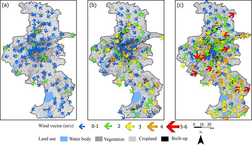
736                                                        S. Chen et al.: A monitoring approach of canopy urban heat island

range (Argüeso et al., 2014), water consumption, and general        rounding environment (Hu et al., 2016; Bassett et al., 2016;
thermal comfort (Salata et al., 2017). Due to its negative im-      Ching et al., 2018; An et al., 2020). Deploying denser ob-
pacts, the UHI effect has become a key challenge in achiev-         servation stations or urban microclimate surveys can to some
ing urban sustainability, and assessing this phenomenon has         extent compensate for the limitation of a coarse spatial reso-
attracted increasing interest over the last decade or so (Cor-      lution. However, such approaches are usually unsuitable for
burn, 2009; Pandey et al., 2014; Malings et al., 2017). In          large-scale studies due to restrictions imposed by certain nat-
general, both background weather conditions (e.g., the wind         ural conditions, social activities, as well as the high cost of
vector and heatwaves) and city-specific characteristics (in-        construction and maintenance (An et al., 2020). For exam-
cluding the presence of urban green space, properties of            ple, mobile transect surveys have been used in many studies
built-up materials, and the intensity of human activity) in-        (Merbitz et al., 2012; Akdemir and Tagarakis, 2014; Hankey
fluence the UHI’s mean intensity and variation (Zhao et al.,        and Marshall, 2015; Al-Ameri et al., 2016; Liu et al., 2017;
2014; Manoli et al., 2019). Concerning these factors, the UHI       Popovici et al., 2018), as they can easily obtain the distribu-
also shows significant intracity variability since urban areas      tion of parameters along a designed route using only a set of
are highly heterogeneous. Therefore, exploring the formation        equipment attached to a mobile vehicle. However, it is rather
and causes of UHIs is crucial for decision-makers involved          costly to obtain observations at a fine resolution, broad cov-
in the planning of urban developments and allocating public         erage, and high synchronicity with such an approach.
resources.                                                             To overcome these possible issues, LST data from aerial
   There are two main approaches to studying UHIs: numeri-          sensors and Earth-observing satellites are commonly em-
cal simulation and observation. Numerical simulation can re-        ployed in UHI studies, and so remote sensing data such as
duce the need for a large number of observations and reveal         those from the Advanced Very High Resolution Radiometer
mechanistic insights by investigating the impacts of cities on      (AVHRR) (Roth et al., 1989; Caselles et al., 1991; Gallo et
meteorological variables (Chun and Guldmann, 2014; Zou et           al., 1993a), Landsat (Chen et al., 2007; Zhou et al., 2015;
al., 2014; Zhang et al., 2015; Taleghani et al., 2016; Li et        Zhao et al., 2016), MODIS (Peng et al., 2012; Zhou et al.,
al., 2020). For instance, Zhang et al. (2015) investigated the      2015; Li et al., 2017; Yang et al., 2018; Chakraborty and
influence of land use/land cover (LULC) and anthropogenic           Lee, 2019), aerial images (Buyadi et al., 2013; Heusinkveld
heat flux (AHF) on the structure of the urban boundary layer        et al., 2014; Yu et al., 2020), and so on (Zhao et al., 2020;
in the Pearl River Delta region, China, through a series of         Gallo et al., 1993b; Qin et al., 2001; Chakraborty et al.,
numerical experiments. However, it is important to acknowl-         2020) are widely used to explain the spatial distribution of
edge that numerical simulation is a simplification of the real      the surface UHI and its relationship with the local environ-
world and cannot replace actual observations. Observational         ment (e.g., LULC). Remote sensing data have good applica-
studies of UHIs are arguably more robust in their findings          tion prospects, as they can provide fine resolution and wide
(Hu et al., 2016; Chakraborty and Lee, 2019; Dewan et al.,          data coverage at times when other ground-based observa-
2021) and can mainly be categorized into the following three        tions cannot. However, due to the influence of precipitation
methods: (1) in situ (field) measurement, (2) mobile mea-           and clouds, the retrieval of LST sometimes can be challeng-
surements, and (3) remote sensing technology.                       ing. In addition, each satellite remote sensing dataset has its
   In situ (field) measurements include conventional mea-           own characteristics (Zhao et al., 2016; Chakraborty and Lee,
surements from national meteorological stations which are           2019). For example, Landsat images have a high spatial reso-
usually located in rural areas and high-density microclimate        lution (30 m) that can show urban block sizes, but the tempo-
observations from experiments or high-density automatic             ral resolution is rather low (16 d). The MODIS LST dataset
sites over various underlying surfaces. It is easy to compare       has the advantage of high temporal resolution (four times
long-term series of air temperature (AT) between urban and          per day), but the spatial resolution is only 1 km (Yang et al.,
rural stations based on meteorological observation data (Liu        2018).
et al., 2006, 2008; Qiu et al., 2008; Yang et al., 2012; Scott         LST derived by satellites has become an important indi-
et al., 2018; Nganyiyimana et al., 2020). With the analysis         cator for exploring variation characteristics of the SUHI, be-
of meteorological data in a long time series, the contribution      cause LST is closely related to the land cover type/structure,
and trend changes of UHI intensity (UHII) can be clearly            population density, anthropogenic heat release, etc., and it
discovered. Meanwhile, however, due to the limitations of           also can significantly influence surface air temperature, wind
meteorological sites in terms of their spatial representation,      field, humidity, and surface fluxes in the urban region (Ho
it is difficult to build a comprehensive understanding of the       et al., 2016; Yang et al., 2019; Li et al., 2020, 2021). How-
spatial distribution of urban thermal environment parameters        ever, the LST can only quantify the SUHI effect, which is
(such as urban canopy temperature, land surface temperature         seriously affected by meteorological factors, e.g., clouds and
(LST) and vegetation) (Liu et al., 2008; Nganyiyimana et al.,       evaporation. In contrast, as an important indicator reflect-
2020). To overcome these limitations, high-density observa-         ing the energy exchange between the atmosphere and land
tion stations are used to explore the spatial distribution of the   in the urban canopy, AT is more representative than LST.
urban thermal environment and its relationship with the sur-        In particular, AT is more related with human health and

Atmos. Meas. Tech., 15, 735–756, 2022                                                 https://doi.org/10.5194/amt-15-735-2022
S. Chen et al.: A monitoring approach of canopy urban heat island 737
ecological changes in cities (Ho et al., 2016). While UHI High-density automatic meteorological observation data,
studies based on AT observed by meteorological sites suffer including AT (with resolution of 0.5◦ on 11 August 2013 and
from limited spatial coverage, which impedes a comprehen- 0.1◦ on 2 September 2015 and 21 July 2017), wind speed,
sive understanding of the influencing factors and causes of and wind direction, at 11:00 LT on the day closest to the
canopy UHI (CUHI). Thus, there is an urgent need to develop satellite transit time, were selected. All weather stations in
rapid, high-spatiotemporal-resolution AT, and refined CUHI operation on those three days were included, numbering 218
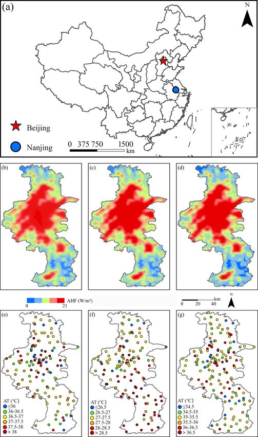
intensity (CUHII) estimation methods to explore the mech- totally and 63, 79, and 76, respectively (Fig. 1). Figure 1
anisms under which anthropogenic factors (e.g., urban land- shows the 2 m AT and LULC on these three days. Compared
use changes, anthropogenic heat emissions, urban morphol- with the LULC, the spatial patterns of AT on these three days
ogy, and size) and natural factors (e.g., meteorological con- are quite different (Fig. 1).
ditions and geographical differences) influence the CUHIs of In addition to global climate change, the influence of hu-
complex and diverse cities. man activities on the CUHI cannot be ignored. Previous stud-
Therefore, in this study, we (1) based on remote sensing ies have pointed out that AHF is closely related to the change
data, AT and wind speed data as well as other environmen- in built-up areas and population density around the stations,
tal information from meteorological observations, retrieved which reflects the fact that the effects from both anthro-
the AT data at a 30 m spatial and 1 h temporal resolution in pogenic emissions and land-use change are related to latent
the study area by using machine learning; (2) calculated the heat flux and sensible heat flux (Zhou et al., 2012; Y. Yang et
CUHII distribution based on the retrieved AT data, and fur- al., 2020a; L. Wang et al., 2020; Zhang et al., 2021). There-
ther explored the shape, intensity, and influencing factors of fore, AHF was retrieved via a physical method (Chen and
the CUHI by combining local LULC, wind vector, and urban Shi, 2012; Chen et al., 2012, 2014) based on 1000 m spa-
morphology data. tial resolution NOAA nighttime lighting data and with local
economic development and energy consumption data, and
the AHF data at the same time in Nanjing were provided
2 Materials and methods by Chen and Shi (2012) and Chen et al. (2012, 2014). Note
that the AHF here varied annually. We expect that AHF dis-
2.1 Study areas
tribution can shape the main morphology of urban thermal
Nanjing, the capital city of Jiangsu province in China, is lo- environment. We cannot get AHF data at diurnal and sea-
cated along the lower reaches of the Yangtze River and, as sonal scales. In future, if we obtain high-temporal-resolution
part of the Yangtze River Delta urban agglomeration, has a AHF data, we will update them in the model. And lastly, the
high level of urbanization. In fact, Nanjing has been expe- digital elevation model (DEM) data (30 m spatial resolution)
riencing rapid urbanization since China’s economic reform used in this study are based on the second version of ASTER-
in 1978. According to the National Bureau of Statistics, the GDEM, which is provided by the Geospatial Data Cloud site,
population in Nanjing increased from 6.13 million in 2000 to Computer Network Information Center, Chinese Academy of
8.34 million inhabitants in 2018. In 2016, the built-up area Sciences (http://www.gscloud.cn, last access: 10 April 2021).
of Nanjing expanded to 773.79 km2 , pushing the city to rank
as the ninth-largest among all Chinese cities (R. Wang et al., 3 Random forest model framework for air temperature
2020). The total GDP in 2020 was about CNY 1.48 trillion, retrieval
ranking ninth among all Chinese cities.
3.1 Construction of random forest model
2.2 Data
The random forest (RF) model is a highly flexible machine
All of the satellite remote sensing data employed in this study learning algorithm that can analyze data with missing val-
are from the geospatial data cloud (https://www.gscloud.cn/, ues or noise and has good anti-interference ability. To date,
last access: 10 April 2021), including those gathered by the the RF model has been widely used as a feature selection
Landsat 8 Operational Land Imager (OLI). OLI has nine tool for high-dimensional data to, for example, identify the
bands, including a coastal band, blue band, green band, red importance of variables and predict or classify related vari-
band, near-infrared band, two shortwave infrared bands, a ables. In this study, an RF model was constructed for each
panchromatic band, and a cirrus band. Due to the low tem- time’s dataset to evaluate the AT using the RF package in R
poral resolution (16 d) of the Landsat 8 OLI dataset and the language.
vulnerability to cloud cover, data from three instances of
cloudless conditions over Nanjing were selected for use in 3.1.1 Data preparation
this paper – namely, 10:43 local time (LT) on 11 August
2013, 2 September 2015, and 21 July 2017. The specific band The process of urbanization will have a significant impact on
ranges and uses of Landsat 8 OLI are shown in Table S1 of CUHIs (Zhou et al., 2015). To comprehensively take into ac-
the Supplement. count the local urban environment, 18 factors were selected
https://doi.org/10.5194/amt-15-735-2022 Atmos. Meas. Tech., 15, 735–756, 2022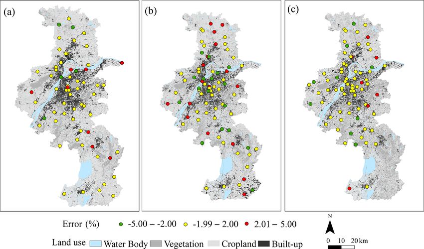
738                                                         S. Chen et al.: A monitoring approach of canopy urban heat island

Figure 1. Anthropogenic heat flux of Nanjing city and locations of high-density automatic meteorological stations in Nanjing with recorded
air temperature: (a) location map of Nanjing in China; (b, e) 11:00 LT on 11 August 2013; (c, f) 11:00 LT on 2 September 2015;
(d, g) 11:00 LT on 21 July 2017.

Atmos. Meas. Tech., 15, 735–756, 2022                                                      https://doi.org/10.5194/amt-15-735-2022
S. Chen et al.: A monitoring approach of canopy urban heat island                                                                 739

as independent variables, including anthropogenic parame-
ters (i.e., AHF), geometric parameters (distance from the city
center, proportion of LULC area, altitude, longitude, lati-
tude, slope, aspect), and physical parameters: proportion of
impervious surface (IS) area, albedo, normalized difference
vegetation index (NDVI), normalized difference built-up in-
dex (NDBI), green normalized difference vegetation index
(gNDVI), soil-adjusted vegetation index (SAVI), and nor-
malized difference moisture index (NDMI). Their sources
and spatial resolution are summarized in Table 1. The in-
version methods for these environmental variables were as
follows: based on Landsat 8 OLI satellite data, the LULC
in Nanjing was divided into four broad categories (built-up,
cropland, vegetation, and water body) by combining a sup-
port vector machine method and visual interpretation. The
remote sensing indices were calculated using corresponding
bands (Yang et al., 2012; Shi et al., 2015). The IS and surface
albedo data were extracted via multi-band information (Son
et al., 2017; Liang, 2001). Then, the geometric center of the
built-up area was calculated as the city center, and the dis-
tances between the meteorological stations and the city cen-
ter were calculated. Slope and aspect were calculated based
on the DEM data using ArcMap 10.2. The methods used for
extracting the IS data and calculating the remote sensing in-
dices and surface albedo are given in Sect. S1, together with
the accuracy of IS and albedo. All the above data (except
for DEM, aspect, and slope) were extracted for each of the
3 years corresponding to the three selected Landsat images.
Taking the data on 21 July 2017 as an example, Fig. 2 shows
the spatial distribution of some of the environmental param-
eters, i.e., IS, distance from city center, LULC, and NDVI,        Figure 2. Spatial distribution of typical environmental variables on
where high spatial consistency between these parameters and        21 July 2017 in Nanjing: (a) impervious surface; (b) distance from
the urban structure can be seen. For example, high-density         city center; (c) LULC; (d) NDVI.
built-up areas correspond closely to high AHF and low veg-
etation cover.
   Due to advection and turbulent transport, neighborhood
surroundings can affect the local temperature (Yang et al.,
2012; Shi et al., 2015). Therefore, a fixed buffer zone was
built surrounding the meteorological stations. Within the
buffer zone of each station the proportion of IS area and that
of each LULC type, and the average values of surface albedo,
AHF, NDVI, NDBI, SAVI, gNDVI, and NDMI were calcu-
lated. Together with longitude, latitude, altitude, and distance
to the city center, these parameters were fed into the RF
model as independent variables, with AT as the target vari-
able. In addition, to find out the optimal size of the buffer
zones for the model, we compared the model performances
for different buffer zone sizes, i.e., buffer zones with a ra-
dius of 500, 1000, 2000, and 5000 m, respectively. Figure 3
summarizes the research framework of this paper.

3.1.2   The 5-fold cross validation
                                                                   Figure 3. Flowchart for constructing the RF model and evaluating
This paper uses the coefficient of determination (R 2 ) and        the CUHII (canopy layer urban heat island).
root-mean-square error (RMSE) as verification indicators.

https://doi.org/10.5194/amt-15-735-2022                                                  Atmos. Meas. Tech., 15, 735–756, 2022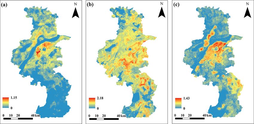
740                                                                       S. Chen et al.: A monitoring approach of canopy urban heat island

Table 1. Independent variables with their sources and spatial resolution.

                                              Parameters                                             Source                                           Spatial
                                                                                                                                              resolution (m)
          Geometric parameters                Proportion of LULC area                                Landsat 8 data                                          30
                                              Latitude and longitude
                                              Distance from the city center                          LULC data
                                              Altitude, slope, and aspect                            DEM data
          Physical parameters                 Proportion of IS area                                  Landsat 8 data                                          30
                                              Albedo
                                              NDVI, NDBI, gNDVI, SAVI, and NDMI
          Anthropogenic parameters            AHF data                                               NOAA nighttime lighting data                         1000
        Notes: DEM, digital elevation model; IS, impervious surface; NDVI, normalized difference vegetation index; NDBI, normalized difference built-up index;
        gNDVI, green normalized difference vegetation index; SAVI, soil-adjusted vegetation index; NDMI, normalized difference moisture index; AHF, anthropogenic
        heat flux.

R 2 indicates the degree of fit between the predicted AT and                            step length, and Mtry from 1 to 16 respectively, with 1 as the
the observed AT, and the RMSE can reflect the credibility of                            step length to traverse all the parameters. Figure 4 presents
the prediction result.                                                                  the R 2 and RMSE values in each 5-fold CV test.
    The cross validation (CV) method can be used to evaluate                               The principle of parameter selection is to choose a simpler
the performance of the RF model (Zheng et al., 2020). In this                           model (smaller Ntree and Mtry) under the premise of good
paper, we employ the 5-fold CV method, in which the en-                                 performance. In the end, the optimal Mtry and Ntree based
tire dataset is randomly divided into five subsets – each time                          on the datasets on 11 August 2013, 2 September 2015, and
four subsets are used to train the RF model, and the remain-                            21 July 2017 were 7 and 200, 10 and 150, and 7 and 50,
ing one is used for validating. After constructing the model,                           respectively.
the validation data are used to calculate the current R 2 and
RMSE, and the process is repeated until each of the 5 folds                             3.2     Model testing
has been used as validation data. The randomness in the pro-
cess of selecting samples for modeling gives the model the                              Table 2 compares the performance of the RF model with dif-
advantage of being robust and highly accurate. With enough                              ferent buffer sizes (500, 1000, 2000, and 5000 m) in the 5-
decision trees, it can ensure that each sample is used as a                             fold CV. The RF model based on the dataset on 11 August
training sample and a test sample, effectively avoiding over-                           2013 and 2 September 2015 within 1 km buffer zones per-
fitting.                                                                                formed best, with an R 2 and RMSE of 0.57 and 0.65 ◦ C, and
                                                                                        0.59 and 0.69 ◦ C, respectively. On 21 July 2017, the R 2 and
3.1.3    Variable selection and model parameter setting                                 RMSE with a 2 km buffer zone were 0.47 and 0.80 ◦ C, re-
                                                                                        spectively, outperforming other buffer sizes. As can be seen
Since not every variable in the model makes a prominent con-                            from Table 2, on 11 August 2013 and 2 September 2015, the
tribution to the performance, deleting those variables that can                         R 2 and RMSE with the 1 km buffer zone were very close to
reduce the prediction accuracy can improve the performance                              those from the optimal buffer size, i.e., the 2 km buffer zone,
and simplify the model. Therefore, the number of variables                              whereas on 21 July 2017, the R 2 and RMSE with the 1 km
should be minimized on the premise of improving or not af-                              buffer zone deteriorated considerably compared to those with
fecting the performance of the model. The contribution of                               the 2 km buffer zone. In addition, according to recent stud-
each variable is judged by two indicators: the percentage                               ies, the effective range that can influence local temperature
increase in mean-square error (%IncMSE) and the percent-                                is within 2 km (Ren and Ren, 2011; Yang et al., 2012; Shi et
age increase in node purity (IncNodePurity). Using the back-                            al., 2015). Therefore, a 2000 m buffer was finally chosen in
ward selection method, the variable with the smallest con-                              this study.
tribution is identified and removed, and the model is re-run.                              In addition, three methods of AT modeling were also com-
These steps are then repeated until only one variable remains.                          pared – two linear regressions – stepwise linear regression
The R 2 and RMSE under different combinations of variables                              (Alonso and Renard, 2019; Mira et al., 2017) and geograph-
were evaluated (Fig. S1).                                                               ically weighted regression (GWR) (L. Wang et al., 2020; Li
   To build an RF model, two important parameters need to                               et al., 2021) – and one nonlinear regression (the RF model;
be set: the number of decision trees (Ntree) and the number                             Alonso and Renard, 2020). A detailed description of the lin-
of variables sampled at each node (Mtry). The RF models                                 ear regression methods is provided in Sect. S2. For each
were established with Ntree from 50 to 1200, with 50 as the                             model, the combination of variables with the largest R 2 and

Atmos. Meas. Tech., 15, 735–756, 2022                                                                           https://doi.org/10.5194/amt-15-735-2022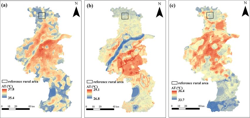
S. Chen et al.: A monitoring approach of canopy urban heat island                                                                   741

Figure 4. The (a–c) R 2 (coefficient of determination) and (d–f) RMSE (root-mean-square error) changes with the parameters Ntree and Mtry
of the model using the dataset on (a, d) 11 August 2013, (b, e) 2 September 2015, and (c, f) 21 July 2017.

Table 2. R 2 and RMSE of the RF model with different buffer radii (500, 1000, 2000, 5000 m). Date format: dd/mm/yyyy.

                                              500 m            1000 m            2000 m           5000 m
                                           R2    RMSE        R2    RMSE        R2    RMSE        R2   RMSE
                                                  (◦ C)             (◦ C)             (◦ C)            (◦ C)
                           11/08/2013     0.33      0.75   0.57      0.65     0.56     0.65    0.36     0.74
                           02/09/2015     0.58      0.70   0.59      0.69     0.57     0.70    0.49     0.76
                           21/07/2017     0.19      0.92   0.17      0.91     0.47     0.80    0.16     0.93

smallest RMSE was selected. Using this approach, eight,                 nonlinear and complex data and suitability for predicting AT
seven, and six variables were selected for the models on                (Zhu et al., 2019; Yoo et al., 2018).
11 August 2013, 2 September 2015, and 21 July 2017, re-
spectively (Table 3). Table 3 also shows the performance of             3.3   Prediction accuracy of RF models
each model based on the dataset within a 2000 m buffer zone.
Compared to the other methods, the RF model achieves bet-               Figure 5 compares the measured AT of the high-density au-
ter R 2 and RMSE, indicating its higher capability in fitting           tomatic stations in the training set or testing set and the pre-

https://doi.org/10.5194/amt-15-735-2022                                                       Atmos. Meas. Tech., 15, 735–756, 2022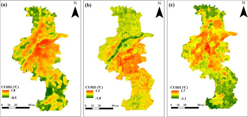
742                                                          S. Chen et al.: A monitoring approach of canopy urban heat island

Table 3. R 2 and RMSE of stepwise regression, GWR (geographi-         Table 4. Importance of input variables for the RF model of AT esti-
cally weighted regression), and the RF model within a 2 km buffer     mation on the three different days. Date format: dd/mm/yyyy.
zone. Date format: dd/mm/yyyy.
                                                                              11/08/2013                     %IncMSE          IncNodePurity
              Stepwise regression         GWR         RF model
                                                                              Water body                             9.23                  4.71
               R2        RMSE )      R2    RMSE      R2    RMSE               NDVI                                   8.38                  4.22
                           (◦ C)            (◦ C)           (◦ C)             NDBI                                   7.15                  7.13
 11/08/2013   0.30          0.69    0.33     0.77   0.56     0.65             IS                                     6.93                  6.46
 02/09/2015   0.47          0.74    0.44     0.82   0.57     0.70             Built-up                               4.19                  2.05
 21/07/2017   0.27          0.90    0.12     0.93   0.47     0.80             Vegetation                             2.35                  1.38
                                                                              AHF                                    0.89                  2.91
                                                                              Cropland                               0.27                  1.70
                                                                              02/09/2015                     %IncMSE          IncNodePurity
dicted AT of the RF model in the 5-fold CV. In general, a
                                                                              Cropland                               5.10                 9.45
large number of scattered points of predicted and observed
                                                                              Distance to city center                4.57                 8.59
AT are clustered around the 1 : 1 line, indicating good per-
                                                                              Water body                             4.00                11.05
formance of the model. In the training set, the average R 2                   NDVI                                   3.18                 5.34
and RMSE of the three models are 0.955 and 0.325 ◦ C, re-                     NDBI                                   2.44                 4.05
spectively. The R 2 and RMSE using data on 11 August                          Built-up                               2.41                 2.78
2013, 2 September 2015, and 21 July 2017 are 0.948 and                        SAVI                                   1.49                 2.67
0.295 ◦ C, 0.954 and 0.310 ◦ C, and 0.963 and 0.369 ◦ C, re-                  Vegetation                             1.44                 2.24
spectively, indicating high model accuracy. The result of the                 IS                                     0.40                 2.59
testing set shows that the average R 2 and RMSE are 0.535                     21/07/2017                     %IncMSE          IncNodePurity
and 0.719 ◦ C, respectively. Among them, the prediction re-
sults achieved on 21 July 2017 are slightly less accurate                     Distance to city center              20.01                 16.22
than those obtained on the other two days. A smaller R 2                      IS                                   18.36                 15.75
                                                                              Vegetation                           11.52                  8.08
and larger RMSE were observed on 21 July 2017 (0.468,
                                                                              NDVI                                  9.89                  3.85
0.802 ◦ C) compared to 11 August 2013 (0.563, 0.655 ◦ C) and
                                                                              gNDVI                                 7.86                  3.28
2 September 2015 (0.574, 0.700 ◦ C). Based on existing re-                    SAVI                                  6.78                  2.38
search (Oh et al., 2020; Venter et al., 2020) and follow-up                   Water body                            6.45                  6.24
discussion (Sect. 4.2.1), it can be concluded that the model
                                                                            Notes: NDVI, normalized difference vegetation index; IS, impervious
performs best outside of the summer months, when the spa-                   surface; AHF, anthropogenic heat flux; DEM, digital elevation model;
tial variation in AT is low and wind velocities are high, cor-              NDBI, normalized difference built-up index; gNDVI, green normalized
                                                                            difference vegetation index; SAVI, soil-adjusted vegetation index.
responding to the model from 2 September 2015. In con-
trast, during the summer months, the performance of the
model constructed with a high spatial variation of AT or low
wind speed conditions decreases slightly, corresponding to            and 21 July 2017, respectively. In detail, most of errors are
the datasets on 21 July 2017 and 11 August 2013.                      concentrated between −0.49 and 0.5 ◦ C over more than half
   Furthermore, we used %IncMSE and IncNodePurity to de-              of all stations for these three days (Fig. S2), and more than
termine the contribution of each variable (Table 4) and to            39.1 %/71.7 %/86.3 % of the total stations exhibit predictions
compare their importance. The NDVI, and the proportion of             with relative errors < 1 %/2 %/3 % (Fig. 6), indicating good
IS, vegetation, and water body area all appeared in the three         performance of RF models for most areas.
models, indicating that vegetation, water bodies, and human
activities have important and universal impacts on the AT             3.4    Model robustness
distribution. The distance to the city center appeared in the
model based on the data on 2 September 2015 and 21 July               To validate robustness of this RF framework and its practical-
2017, and ranked high, implying the impact of urbanization            ity at a long period, hourly meteorological AT observations
on the heat island.                                                   during August 2013, September 2015, and July 2017, and
   The absolute error for RF prediction is defined as dif-            corresponding environment variables were chosen to estab-
ference in predicted AT and observed AT at each weather               lish the RF model. The temperature differences in a month
station(See Fig. S2). The relative error is defined as that           are larger, showing more complicated situations. For 5-fold
absolute error divided by observed AT, which is shown in              CV, a scatterplot of predicted and observed air temperature
Fig. 6. In general, the mean relative (absolute) errors by            is given in Fig. 7, showing that the mean RMSEs are 0.75,
all stations are 0.07 % (0.014 ◦ C), 0.04 % (−0.025 ◦ C), and         0.52, and 0.59 ◦ C, and R 2 values are 0.98, 0.99, and 0.99, re-
0.05 % (0.003 ◦ C) on 11 August 2013, 2 September 2015,               spectively, in August 2013, September 2015, and July 2017.

Atmos. Meas. Tech., 15, 735–756, 2022                                                         https://doi.org/10.5194/amt-15-735-2022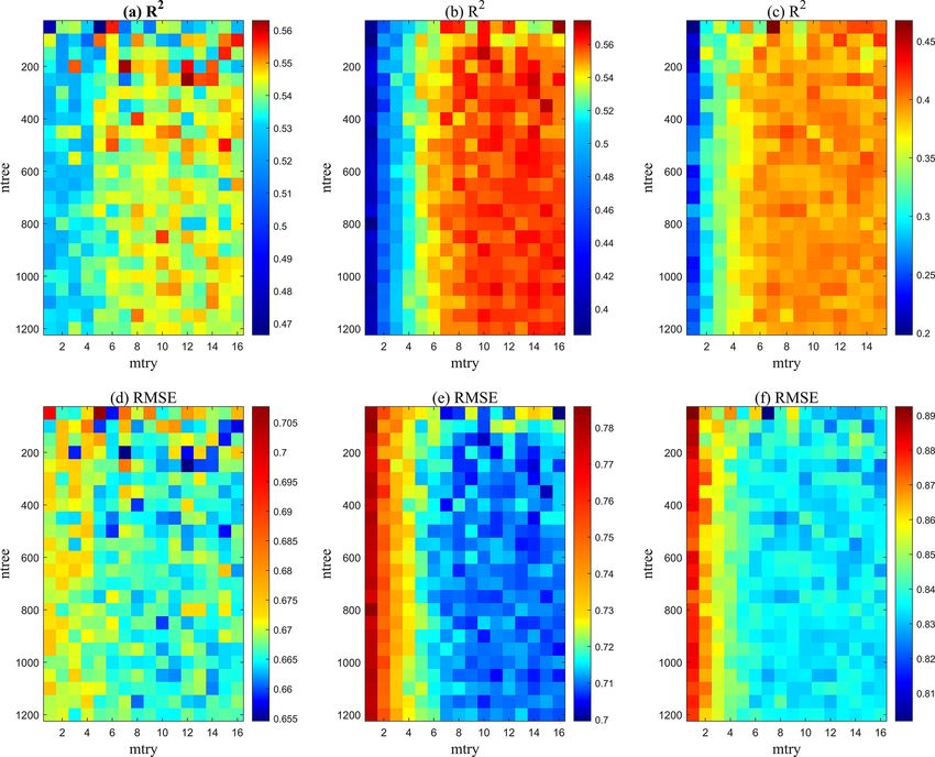
S. Chen et al.: A monitoring approach of canopy urban heat island                                                                      743

Figure 5. Scatterplot of predicted and observed air temperature: 5-fold cross validation (CV) for the training set on (a) 11 August 2013,
(b) 2 September 2015, and (c) 21 July 2017; 5-fold CV for the testing set on (d) 11 August 2013, (e) 2 September 2015, and (f) 21 July 2017.

Figure 6. The predicted relative error of the air temperature by random forest: (a) 11 August 2013; (b) 2 September 2015; (c) 21 July 2017.

In general, for 1-month samples, the mean R 2 reached 0.986             4     Refined CUHII assessment in Nanjing
and RMSE was 0.620 ◦ C. Note that most of the points are
clustered around the 1 : 1 line and the performance is better           4.1    Refined AT and CUHII and comparison with LST
than the model using 1 d samples. The accuracy in August                       distribution
2013 is the lowest because that resolution of observed AT is
0.5 ◦ C in this month, while it is 0.1 ◦ C in other two months,         After establishing the model, a 2 km buffer area was created
so the performance is the worst among three months.                     for each 30 m resolution pixel and the same 18 independent
                                                                        variables were calculated. The constructed RF model took
                                                                        these pixel-wise variables as input and output AT for each

https://doi.org/10.5194/amt-15-735-2022                                                       Atmos. Meas. Tech., 15, 735–756, 2022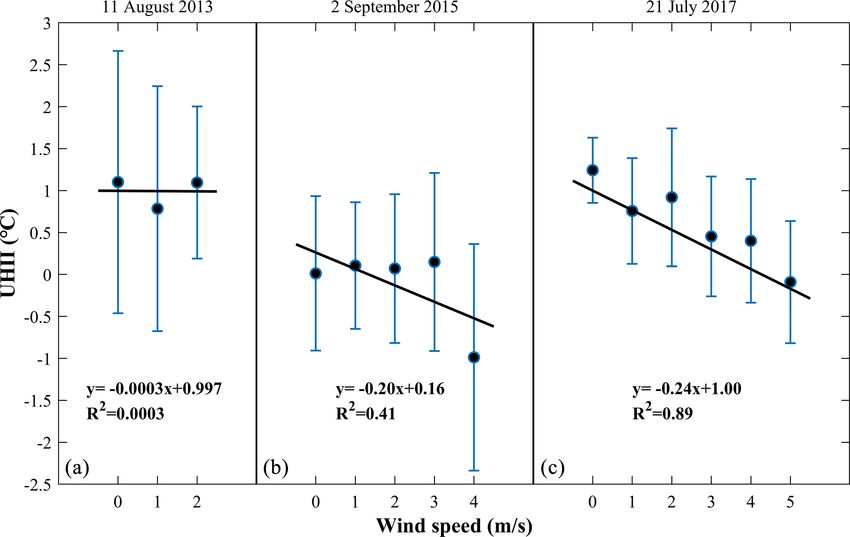
744 S. Chen et al.: A monitoring approach of canopy urban heat island
Figure 7. Scatterplot of predicted and observed air temperature using data in a 1-month 5-fold CV for the testing set on (a) August 2013,
(b) September 2015, and (c) July 2017.
pixel, and hence we obtained the RF model–predicted AT was found to be generally stronger than that in autumn and
map at 30 m resolution (Fig. 8). LST is also a physical mani- winter. The difference between the maximal heat island and
festation of surface energy and moisture flux exchange be- cold island intensity on 21 July 2017 was 2.8 ◦ C, the largest
tween the atmosphere and the biosphere. Previous studies among the three cases. Generally, the densely populated cen-
point out that there is a relationship between LST and AT tral city area has a large proportion of IS area, large anthro-
(Mutiibwa et al., 2015; Benali et al., 2012); therefore, Fig. 9 pogenic heat emissions, and higher AT and LST, showing
shows the LSTs of Nanjing on these days, which were re- an obvious UHI phenomenon (Figs. 8, 9, and 10). However,
trieved by using Google Earth Engine. CUHII is an impor- in urban areas with high vegetation coverage or large water
tant indicator to quantify the UHI effect, which is usually bodies, the AT and LST decrease with weakened CUHII. The
defined as the difference in AT at the same level between ur- AT and LST gradually decrease from the city center to the
ban and rural areas (Y. Yang et al., 2020b; Nganyiyimana et suburbs. Suburban areas, which are covered by more vegeta-
al., 2020), as follows: tion and water bodies, have significantly lower AT and LST
than central urban areas. At the boundary of the central city,
CUHII = T − Trural , (1) high-AT areas and heat islands extend outward along built-up
areas and roads (Figs. 8, 9, and 10).
where T is the predicted AT in each pixel and Trural is the Against different weather backgrounds, the spatial distri-
average AT in the reference rural area. A square area of size butions of AT and CUHII exhibit heterogeneity in urban Nan-
10 km × 10 km was selected as the reference rural area in the jing on different days. The high-AT area on 11 August 2013
northern part of Nanjing (Valmassoi and Keller, 2021). It was extended from the city center to a wide range, and the ex-
far from the city center and barely impacted by the UHI ef- treme value of AT was the highest (Fig. 8a), corresponding to
fect (Fig. 8). The average AT in each reference rural area the strongest CUHI (Fig. 10a). Combined with Fig. 2, we can
was 36.0, 27.8, and 34.7 ◦ C on these three days, respectively. see only a small range of vegetation coverage and water bod-
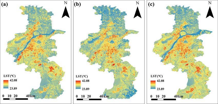
Then, the CUHII distribution in Nanjing was calculated ac- ies in the central urban area, so the CUHII decreased slightly.
cording to Eq. (1) (Fig. 10). Only in the suburban water body and farmland areas were
Figure 8 shows that the AT on 11 August 2013 and 21 July there large cold island areas, and only on this day, the dis-
2017 was higher and that the AT ranges were 35.4–37.8 tribution of LST corresponds to that of AT. On 2 September
and 33.6–36.4 ◦ C, respectively. The corresponding CUHII 2015, the high-AT area was relatively small to the north of the
was strong, with more than 1.5 ◦ C in the downtown area Yangtze River. The AT on the Yangtze River was the lowest
(Fig. 10). On 2 September 2015, the AT range was 26.8– (Fig. 8b), with the strongest cold island here (Fig. 10b). The
29.1 ◦ C (Fig. 8) and the CUHI was slightly weaker, with high-AT area extended from the central city to the south, and
the maximum value at only 1.3 ◦ C (Fig. 10). In contrast, the the cold islands in the southern water body and vegetation-
LSTs are higher, ranging from 26.2–44.1, 21.3–44.1, and covered areas were not significant. On 21 July 2017, the dis-
23.9–42.1 ◦ C on 11 August 2013, 2 September 2015, and tribution of the heat island was the opposite. There was a
21 July 2017, respectively (Fig. 9). The three images from large area of high AT to the north of the Yangtze River, and
different seasons and different weather backgrounds led to the cooling effect of the Yangtze River was weak (Fig. 8c).
significant differences in CUHII, while LST differences are Meanwhile, the AT in the southern suburbs dropped signif-
marginal. On 2 September 2015, the overall CUHI was the icantly, and cold islands widely spread in water body and
weakest among the three days. Consistent with a previous cropland areas (Fig. 10c). Compared with the distribution of
study (R. Wang et al., 2020), the summer CUHI in Nanjing
Atmos. Meas. Tech., 15, 735–756, 2022 https://doi.org/10.5194/amt-15-735-2022S. Chen et al.: A monitoring approach of canopy urban heat island 745 Figure 8. Spatial distribution of AT in Nanjing and the reference rural area: (a) 11 August 2013; (b) 2 September 2015; (c) 21 July 2017. Figure 9. Spatial distribution of the LST in Nanjing: (a) 11 August 2013; (b) 2 September 2015; (c) 21 July 2017. CUHII on 11 August 2013, the AT over the water bodies and et al., 2016; Long et al., 2020). The LULC types in these hills in the northeast of the central city was lower, forming a periods are similar, so the LST differences are marginal. large and strong cold island area. To further explore the intensity and coverage of the CUHI However, note that the distributions of LST at these three on different days, the area (km2 ) occupied by different lev- times are similar, and they are all strongly related to urban els of CUHII on the three different days was calculated (Ta- form and LULC (Li et al., 2021). This is because different ble 5). The CUHI area on 11 August 2013 accounted for factors caused different spatial distribution between LST and 84.1 % and the area of the CUHII in the range of 1–1.5 AT. Ground transfers heat to the air through radiation, con- and 1.5–2 ◦ C was 1486.89 and 82.96 km2 , respectively. On duction, and convection after absorbing solar energy, which 2 September 2015, the CUHI area accounted for 80.2 % and is the main source of heat in the air (Hong et al., 2018; Khan the CUHII area at 0–0.5 ◦ C accounted for 57.0 %, concentrat- et al., 2020). While LST is directly heated by solar energy, ing in this range, while that at 1–1.5 ◦ C was only 56.97 km2 . which is more sensitive to emissivity, surface material and The strongest cold island was lower than −1 ◦ C, and the humidity, which are related to LULC, tend to have greater overall CUHI effect was relatively weak. On 21 July 2017, temperature differences for different LULC types (Janatian https://doi.org/10.5194/amt-15-735-2022 Atmos. Meas. Tech., 15, 735–756, 2022
746 S. Chen et al.: A monitoring approach of canopy urban heat island
Figure 10. Spatial distribution of the CUHII in Nanjing: (a) 11 August 2013; (b) 2 September 2015; (c) 21 July 2017.
Table 5. Area occupied by different levels of urban heat island intensity on different days (km2 ). Date format: dd/mm/yyyy.
CUHII level (◦ C) −1.5 to −1 −1 to −0.5 −0.5 to 0 0 to 0.5 0.5 to 1 1 to 1.5 1.5 to 2
11/08/2013 0.00 0.15 1047.43 1517.19 2446.03 1486.89 82.96
02/09/2015 0.02 192.13 1109.89 3751.88 1472.26 56.97 0.00
21/07/2017 0.23 232.52 1005.04 2670.11 2040.98 634.13 0.14
the CUHI area accounted for 81.2 %, and the area where the scending motion, and stable weather, leading to increased
CUHII was greater than 1.5 ◦ C was only 0.14 km2 . CUHI strength (Fig. 10a) (Wang et al., 2021). On 2 Septem-
ber 2015, the average wind speed was 1.53 m s−1 , which
4.2 Potential drivers of CUHII was a significant increase (Fig. 11b). The overall northwest-
erly wind direction led to the CUHII being lower than that
According to previous studies, three factors – the wind vector on 11 August 2013. Indeed, it has been noted in previous
field (He, 2018), LULC (Cao et al., 2018; R. Wang et al., work that the wind direction will significantly affect the
2020) and the urban structure (Shahmohamadi et al., 2011; position and shape of a heat island (Bassett et al., 2016),
Li et al., 2020) – are the most important influencing factors and in the present study the northwesterly winds resulted in
of CUHIs. In this section, we explore these three drivers of the CUHI extending from the built-up area to the southeast
CUHI in Nanjing. (Fig. 10b) whilst weakening significantly in the northwest.
On 21 July 2017, the average wind speed reached 3.07 m s−1 ,
4.2.1 Relationship between CUHII and the wind vector with a southwesterly wind direction (Fig. 11c). The CUHI ef-
field fect weakened accordingly, extending to the northeast in the
downward wind, and the CUHI was significantly weakened
The horizontal air flow has a significant impact on the in- in the southwest (Fig. 10c).
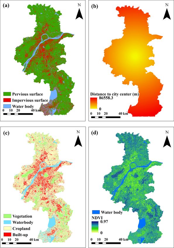
tensity and shape of the CUHI (He et al., 2021). Figure 11 On all three days, the wind speed in the suburban areas
shows the wind vector field observed by weather stations on was higher than that in the central city, and this is because
the three days analyzed in our study. there is no shelter provided by tall and dense buildings in
On 11 August 2013, the average wind speed at the sta- the suburban areas, which is conducive to cooling from air
tions was 0.70 m s−1 , most of which recorded calm wind convection and therefore a weakening of the CUHII (P. Yang
(0–0.2 m s−1 ) or soft wind (0.3–1.5 m s−1 ) (Fig. 11a). The et al., 2020). That said, records show that, surprisingly, the
main reason for this was that Nanjing was continuously con- boundary-layer mean wind speed in a city can be higher than
trolled by the western Pacific subtropical high at this time and its rural counterpart. On the one hand, Nanjing is traversed
was therefore experiencing a continuous heatwave – condi- by the Yangtze River, and the central city surrounds a large
tions that are usually associated with low wind speeds, de-
Atmos. Meas. Tech., 15, 735–756, 2022 https://doi.org/10.5194/amt-15-735-2022S. Chen et al.: A monitoring approach of canopy urban heat island 747
Figure 11. Wind vector field in Nanjing on (a) 11 August 2013, (b) 2 September 2015, and (c) 21 July 2017.
area of water, wherein the low surface roughness of the water 2 September 2015, the average wind speed was 1.53 m s−1 .
is conducive to air convection. On the other hand, channel- Due to the combined effect of horizontal advection cooling
ing/the Venturi effect might be an important factor. When and heat transfer, an upwind cold island appeared and, mean-
the prevailing wind is parallel to the axis between build- while, the downwind area received heat from the upwind area
ings, it will be forced to enter between the buildings, result- and the CUHII increased significantly (Figs. 10b and 11b).
ing in higher wind pressure, which increases the wind speed On 21 July 2017, the average wind speed was 3.07 m s−1 ,
(Droste et al., 2018). and the upwind CUHII also weakened (Figs. 10c and 11c).
In order to quantify the relationship, the average CUHII Downwind, however, the urban heat convection was the dom-
and standard deviation under different wind speeds at various inant factor, which reduced the CUHII in some areas.
meteorological stations were calculated (Fig. 12). On 11 Au- In contrast, CUHII distribution is in good agreement with
gust 2013, the maximum wind speed was 2 m s−1 , which LST distribution on 11 August 2013, while the large pattern
bore no significant relationship with the CUHII (Fig. 12a). difference during the other two days (Figs. 9 and 11). This
On 2 September 2015 and 21 July 2017, the maximum wind is because calm wind on 11 August 2013 cannot induce hor-
speed reached 5 and 6 m s−1 , respectively, which showed a izontal advection of urban heat; therefore, spatial distribu-
significant negative correlation with the CUHI (Fig. 12b and tions of LST and AT are well matched in this day. However,
c). The greater the wind speed, the more significant the neg- under large wind conditions (e.g., larger wind speeds on both
ative correlation. 2 September 2015 and 21 July 2017), there is obvious urban
There are two aspects concerning the influence of air con- heat island advection (Bassett, et al., 2016), resulting in dif-
vection on CUHIs. On the one hand, air convection will fa- ferent patterns between CUHII and SUHI during these two
cilitate horizontal advection cooling between urban and rural days (Figs. 9 and 11).
areas, thereby weakening the CUHI (Brandsma et al., 2003).
The greater the wind speed, the more significant the cool- 4.2.2 Relationship between CUHII and LULC
ing effect (Fig. 12). On the other hand, horizontal convection
transfers heat from the upwind to the downwind area, weak- LULC also has a significant impact on CUHII (Li et al.,
ening the upwind CUHII and strengthening the downwind 2020; Zong et al., 2021) and LST (Yang et al., 2018; Li
CUHII (Bassett et al., 2016) (Figs. 10 and 11). Under dif- et al., 2021). The average values and standard deviation of
ferent wind speeds, the synergy of these two aspects differs CUHII were calculated for each LULC type on the three days
significantly. On 11 August 2013, the average wind speed (Fig. 13). On 11 August 2013, the CUHII in the built-up area
was the smallest among the three days at only 0.7 m s−1 , and was the strongest, exceeding 1.1 ◦ C, and in the water body ar-
there was no uniform wind direction, corresponding to the eas it was the weakest at only 0.22 ◦ C (Fig. 13a). On 21 July
strongest CUHI. The distribution of the CUHI was highly 2017, the CUHII in the built-up area was the strongest at
correlated with that of built-up areas (Figs. 10a and 11a). On 0.62 ◦ C, and in the vegetation areas it was the weakest at
0.24 ◦ C (Fig. 13b). The CUHII on these two days was high-
https://doi.org/10.5194/amt-15-735-2022 Atmos. Meas. Tech., 15, 735–756, 2022748 S. Chen et al.: A monitoring approach of canopy urban heat island
Figure 12. Relationship between CUHII and wind speed around all meteorological stations on (a) 11 August 2013, (b) 2 September 2015,
and (c) 21 July 2017. The black dots represent the mean canopy UHII; error bars indicate the uncertainties of 1 standard deviation from the
mean.
est in the built-up area, followed by cropland, and then water ble heat flux and reduce the AT (Sect. 4.2.1). There-
bodies and vegetation. On 2 September 2015, the CUHII in fore, LULC and air convection will jointly enhance or
the built-up area was the strongest at 0.32 ◦ C, while it was weaken the CUHII.
the weakest at −0.06 ◦ C in the water body areas (Fig. 13c).
Different LULC types have different effects on AT due to On 11 August 2013, the average wind speed and the differ-
their own intrinsic physical properties, mainly reflected in ence in wind speed between different LULC types were small
three aspects: and so was the difference in sensible heat flux. The differ-
ence in radiation and sensible heat flux was the main factor.
1. Due to the good thermal conductivity and small specific On 21 July 2017, the average wind speed was the highest,
heat capacity of the surface material in the built-up area, and the synergy in the three aspects led to the CUHII over
the ability to absorb shortwave radiation during the day different LULC types being highest in the built-up area, fol-
is stronger than that of other land uses. The LST is sig- lowed by cropland, vegetation, and then water bodies. On
nificantly higher than that of the suburbs, and therefore 2 September 2015, the CUHII was highest in the built-up
the atmosphere is easily heated (Hong et al., 2018). areas, followed by vegetation, cropland, and then water bod-
ies. This was due to the influence of low wind speeds, which
2. Due to sufficient water availability in cropland and would have produced heat transfer and made the CUHII shift
vegetation-covered areas, evaporation will increase the from the built-up area to other LULC types (Sect. 4.2.1).
latent heat flux and cooling effect (Zhao et al., 2020;
Zheng et al., 2018). In contrast, the surface humidity of 4.2.3 Relationship between CUHI and urban structure
the built-up area is low, with low corresponding latent
heat flux. The difference in latent heat flux will increase Human activities and urbanization have a significant impact
the difference in LST and AT between urban and ru- on the spatial distribution of UHI (Shahmohamadi et al.,
ral areas. The latent heat flux of the water bodies is the 2011; Li et al., 2020). To explore this influence, concentric
largest, and the cooling effect is the most obvious. rings with various radii (5, 10, 15, 40 km) were created sur-
rounding the city center. Within each ring, the average values
3. There is a significant correlation between LULC and and error ranges of AHF and CUHII, along with the average
wind speed (Chen et al., 2020). Areas with tall build- proportion of built-up area, were calculated. Figure 14 shows
ings in built-up areas have high surface roughness and that the CUHII, AHF, and proportion of built-up area all sig-
low wind speed, whereas water bodies have low surface nificantly decrease with increasing distance to the city center.
roughness and high wind speed. The surface roughness From a longitudinal perspective, the AHF and the propor-
of vegetation-covered areas and cropland is somewhere tion of built-up areas both increased year by year. The built-
between. The air convection will increase the sensi- up areas of Nanjing on the three days were 982.78, 1076.19,
Atmos. Meas. Tech., 15, 735–756, 2022 https://doi.org/10.5194/amt-15-735-2022S. Chen et al.: A monitoring approach of canopy urban heat island 749 Figure 13. Mean CUHII and standard deviations over different LULC on (a) 11 August 2013, (b) 2 September 2015, and (c) 21 July 2017. Figure 14. Changes in air temperature, AHF, and the proportion of built-up areas with distance from the city center on (a) 11 August 2013, (b) 2 September 2015, and (c) 21 July 2017. Thick lines represent mean values, while shaded regions are the uncertainties of 1 standard deviation from the mean. https://doi.org/10.5194/amt-15-735-2022 Atmos. Meas. Tech., 15, 735–756, 2022
750                                                         S. Chen et al.: A monitoring approach of canopy urban heat island

and 1220.36 km2 , respectively. The proportion of built-up             1. Statistical methods (Prihodko and Goward, 1997;
areas beyond 20 km to the city center increased, especially               Alonso and Renard, 2020; Li et al., 2021): statistical
within the range of 20–25 km. The AHF also showed the                     models of environmental factors and temperature are
same trend, which within the range of 20–25 km even ex-                   established to evaluate the AT, such as multiple linear
ceeded that in the range of 15–20 km on 2 September 2015                  regression models, partial least-squares regression, and
and 21 July 2017. This shows that built-up areas and hu-                  GWR. In previous study (Alonso and Renard, 2020),
man influence were spreading from the city center to the sur-             two methods of AT prediction (namely, stepwise lin-
rounding areas during this period. However, the intensity and             ear regression and GWR) were compared with the RF
range of the CUHI did not increase with this trend, because               model. The RF model has the highest accuracy and ef-
the wind field and weather background have a stronger influ-              fectively avoids the problem of autocorrelation by fil-
ence on CUHI than urbanization (Hong et al., 2018; Zong et                tering variables, which is consistent with previous work
al., 2021).                                                               (Yoo et al., 2018; Zhu et al., 2019) and our present
                                                                          work, while conventional statistical methods, in addi-
                                                                          tion, cannot effectively solve nonlinear problems (Oh et
5   Discussion                                                            al., 2020).

Based on the RF model and combined with local environ-                 2. Temperature–vegetation index method (VTX) (Stisen et
ment and background weather data, the pattern and causes of               al., 2007; Vancutsem et al., 2010): this refers to inver-
CUHIs can be analyzed in detail. On 11 August 2013, Nan-                  sion using the relationship between AT, LST, and veg-
jing experienced a heatwave, with almost no horizontal con-               etation index under the premise that the temperature of
vection of air (Fig. 11a). In dry areas, such as built-up areas,          a dense vegetation canopy is similar to the AT. While
the latent heat flux remained unchanged, but the high reflec-             VTX only indicates the relationships between underly-
tivity of the surface raised the AT. In the heatwave period, the          ing surface, LST, and AT. In fact, there are many factors
higher AT increased the latent heat flux in rural areas (Khan             that can affect AT, e.g., anthropogenic heat, altitude, and
et al., 2020). For example, vegetation and water bodies alle-             distance to city. Ignoring these factors, the accuracy of
viated the increase in AT in rural areas. This combined effect            VTX method was low (Stisen et al., 2007). In contrast,
exacerbated the difference in AT between the urban and rural              our RF model input multiple variables, including more
areas, making the overall CUHI the strongest (Nganyiyimana                affecting AT factors.
et al., 2020; Meili et al., 2021). In Fig. 10a, it can be seen that
the cooling efficiency of vegetation in the urban area was not         3. Physical model methods: this category mainly consti-
high and the coverage of the cooling area was small. This is              tutes the energy balance method (Yang et al., 2018),
because the stomata of leaves would have been closed under                which refers to the study of AT inversion using the prin-
high AT and dry weather, resulting in reduced evapotranspi-               ciple of energy balance. The physical model approach
ration and increased AT (Manoli et al., 2019). On 2 Septem-               is relatively complex, and the performance is highly
ber 2015, northwesterly winds prevailed (Fig. 11b), and there             dependent on the understanding of the mechanism af-
was abundant water vapor over the hills of northeast Nan-                 fecting AT, which can only address specific problems,
jing and over the Yangtze River. The increase in latent heat              while the RF framework in this paper is relatively sim-
flux and horizontal convection cooling lowered the CUHII.                 ple, comprehensive, and suitable for different weather
Cold islands even appeared to the north of the Yangtze River.             backgrounds.
The CUHII in the southeast direction was strong (Fig. 10b),
which was mainly affected by the heat transport of the pre-            4. Machine learning methods (Venter et al., 2020): predic-
vailing winds (Chuanyan et al., 2005), causing the CUHI to                tions are made by establishing models of various vari-
shift toward the downwind area. On 21 July 2017, south-                   ables and AT, such as RF models or neural networks.
westerly winds prevailed in Nanjing, with high wind speed,                Compared with other machine learning methods such as
decreasing the CUHII in the upwind region (Figs. 10c and                  neural networks (Astsatryan et al., 2021), the RF model
11c). However, there were large areas of vegetation coverage              has better noise immunity and is suitable for small sam-
in the range of 10–20 km in the downwind region, where was                ple sizes in this study. Other machine learning meth-
affected by the combined effects of land use and horizontal               ods usually require a lot of data with little noise, so
advection cooling, leading to lower CUHII there than that of              the data cleaning before modeling will take more time.
20–30 km. This also confirms the conclusion (Bassett et al.,              In future, we would like to compare different machine
2016) that the upwind horizontal advection cooling has the                learning methods to come up with a consistently well-
strongest correlation with the weakening of the CUHI effect,              performing model, e.g., SVM and ANN. We will also
and that the downwind region is affected by the wind speed.               use stacking ensemble strategy to combine the advan-
   There are four main methods for retrieving AT for CUHII                tages of different models and get the best prediction re-
assessment:                                                               sults.

Atmos. Meas. Tech., 15, 735–756, 2022                                                  https://doi.org/10.5194/amt-15-735-2022
S. Chen et al.: A monitoring approach of canopy urban heat island 751
Figure 15. Spatial distribution of canopy urban heat island intensity (CUHII) in Nanjing during a heatwave period: (a) 12 August 2013;
(b) 13 August 2013; (c) 14 August 2013.
The RF prediction framework proposed in this work not 6 Conclusions
only can dynamically predict CUHII in detail and high fre-
quency within highly heterogeneous cities but can also be Taking Nanjing as an example and using remote sensing data
built against different weather backgrounds, mainly because with data from local weather stations, parameters to charac-
the environmental parameters entered into the model are rel- terize the urban environment were constructed, e.g., anthro-
atively stable within a certain period (such as the same month pogenic parameters (i.e., AHF), geometric parameters (dis-
or season). As long as the environmental parameters are ac- tance from city center, proportions of LULC types by area,
quired once, they can be combined with the AT data in real altitude, and latitude and longitude, slope, and aspect), and
time to establish the RF model, and the spatial distribution physical parameters (proportion of IS, surface albedo, NDVI,
characteristics of CUHII with high temporal and spatial res- NDBI, SAVI, gNDVI, and NDMI). A 2 km buffer zone was
olution can be obtained. For instance, we randomly predicted created around the meteorological stations, and the observed
the 30 m resolution AT and spatial distribution of CUHII environmental parameters were extracted. A refined assess-
(Fig. 15) with the wind vector field (Fig. S3) during the heat- ment framework of CUHII was then established by using
wave period of 12–14 August 2012, thereby supporting those random forest model with observed AT and environmental
involved in making decisions with respect to urban climate, variables.
urban planning, and urban energy consumption. Particularly, Results showed that the correlation coefficient between
the potential that our proposed model can be used cross a the predicted and observed AT was 0.731, and the average
short period as most of the environmental parameters fed to RMSE was 0.719 ◦ C, indicating the high accuracy of the RF
the model probably can remain stable for some time, e.g., model. Based on 1-month samples, the R 2 reached 0.986
1 month or even longer. and RMSE was 0.620 ◦ C. Finally, the high-spatial-resolution
Due to changes in local weather conditions (e.g., pre- (30 m) CUHII distribution was analyzed. It was found that
cipitation and cloud cover), however, there are various the shape of the CUHII was highly correlated with the spa-
satellite-based LST samples and LST is usually dynamical in tial distribution of AHF and built-up area under calm wind
1 month, leading to uncertainties in predicting AT; therefore, conditions. Under the prevailing wind conditions, the CUHII
LST is not suitable to be an input variable for our present should be discussed separately in upwind and downwind ar-
model of CUHII. Except for human activities and LULC, the eas divided by the central city. In the upwind area, there was
background weather conditions (such as heatwaves, air pol- a significant negative correlation between the wind speed and
lution, atmospheric circulation, and cloud cover) are also ex- CUHII. The higher the wind speed, the more obvious the
tremely important (Bassett et al., 2016; P. Yang et al., 2020; negative correlation. In the downwind area, horizontal con-
Khan et al., 2020), which should be introduced to improve vection cooling was found to be the leading factor under high
the RF model of CUHII. wind speed weather, and heat transfer was the leading fac-
tor under low wind speed weather. The combined effects of
https://doi.org/10.5194/amt-15-735-2022 Atmos. Meas. Tech., 15, 735–756, 2022You can also read