Sentinel-1 observation frequency significantly increases burnt area detectability in tropical SE Asia - IOPscience
←
→
Page content transcription
If your browser does not render page correctly, please read the page content below
Environmental Research Letters

LETTER • OPEN ACCESS

Sentinel-1 observation frequency significantly increases burnt area
detectability in tropical SE Asia
To cite this article: Joao M B Carreiras et al 2020 Environ. Res. Lett. 15 054008

View the article online for updates and enhancements.

                                This content was downloaded from IP address 46.4.80.155 on 02/11/2020 at 05:52
Environ. Res. Lett. 15 (2020) 054008                                                         https://doi.org/10.1088/1748-9326/ab7765

                              LETTER

                              Sentinel-1 observation frequency significantly increases burnt area
OPEN ACCESS
                              detectability in tropical SE Asia
RECEIVED
22 August 2019
                              Joao M B Carreiras1          , Shaun Quegan1 , Kevin Tansey2               and Susan Page2
REVISED                       1
14 February 2020
                                  National Centre for Earth Observation, University of Sheffield, Sheffield, United Kingdom
                              2
                                  Centre for Landscape and Climate Research, School of Geography, Geology & the Environment, University of Leicester, Leicester, United
ACCEPTED FOR PUBLICATION
                                  Kingdom
18 February 2020
PUBLISHED
                              E-mail: j.carreiras@sheffield.ac.uk
29 April 2020
                              Keywords: burnt area, tropics, Sentinel-1, radar, machine learning, Indonesia
                              Supplementary material for this article is available online
Original content from this
work may be used under
the terms of the Creative
Commons Attribution 4.0
licence.                      Abstract
Any further distribution of   Frequent cloud cover in the tropics significantly affects the observation of the surface by satellites. This
this work must maintain
attribution to the            has enormous implications for current approaches that estimate greenhouse gas (GHG) emissions
author(s) and the title of
the work, journal citation
                              from fires or map fire scars. These mainly employ data acquired in the visible to middle infrared bands
and DOI.                      to map fire scars or thermal data to estimate fire radiative power and consequently derive emissions.
                              The analysis here instead explores the use of microwave data from the operational Sentinel-1A (S-1A)
                              in dual-polarisation mode (VV and VH) acquired over Central Kalimantan during the 2015 fire
                              season. Burnt areas were mapped in three consecutive periods between August and October 2015
                              using the random forests machine learning algorithm. In each mapping period, the omission and
                              commission errors of the unburnt class were always below 3%, while the omission and commission
                              errors of the burnt class were below 20% and 5% respectively. Summing the detections from the three
                              periods gave a total burnt area of ∼1.6 million ha, but this dropped to ∼1.2 million ha if using only a
                              pair of pre- and post-fire season S-1A images. Hence the ability of Sentinel-1 to make frequent
                              observations significantly increases fire scar detection. Comparison with burnt area estimates from
                              the Moderate Resolution Imaging Spectroradiometer (MODIS) burnt area product at 5 km scale
                              showed poor agreement, with consistently much lower estimates produced by the MODIS data-on
                              average 14%–51% of those obtained in this study. The method presented in this study offers a way to
                              reduce the substantial errors likely to occur in optical-based estimates of GHG emissions from fires in
                              tropical areas affected by substantial cloud cover.

                              1. Introduction                                                        temporal resolution satellite data (Gregoire et al 2003,
                                                                                                     Simon et al 2004, Silva et al 2005, Miettinen et al 2007,
                              Data acquired by orbital platforms are the only way of                 Giglio et al 2009, 2013, Sedano et al 2013). Further-
                              routinely, consistently and affordably observing and                   more, ongoing projects are providing global and
                              monitoring land processes at large spatial and long                    repetitive burnt area mapping and derived emissions,
                              temporal scales (Harris et al 2012, Hansen et al 2013,                 e.g. the Global Fire Emissions Database (GFED4;
                              Tyukavina et al 2015, Reiche et al 2016). As a result,                 http://globalfiredata.org) (van der Werf et al 2010,
                              estimates of carbon released by fires rely on burnt area                Randerson et al 2012, Giglio et al 2013) and the
                              mapping (Giglio et al 2013), identification of hotspots                 European Space Agency’s (ESA) Climate Change
                              (Randerson et al 2012) or estimates of fire radiative                   Initiative-Fire (CCI-Fire; http://esa-fire-cci.org/)
                              power output (Wooster et al 2012) from satellite data.                 (Chuvieco et al 2016). Most of the fire activity is
                              Currently, the vast majority of methods to map burnt                   observed across the tropics, either as a consequence of
                              areas rely on automatic or semi-automatic processing                   local livelihoods (shifting agriculture in Africa) or land
                              of optical data from high or moderate spatial and                      clearing for agriculture (South America and Southeast

                              © 2020 The Author(s). Published by IOP Publishing Ltd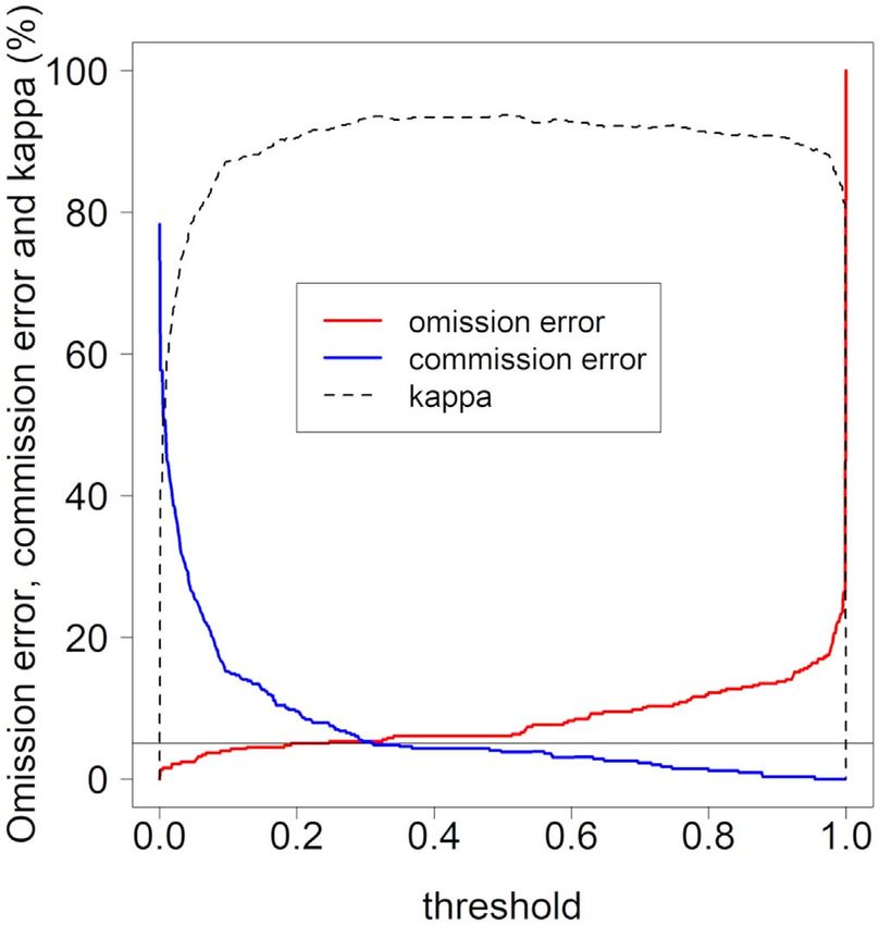
Environ. Res. Lett. 15 (2020) 054008
Asia) (Lambin et al 2003). In these regions, frequent detected at lower frequencies. Lohberger et al (2018)
cloud cover and haze and smoke from the fire activity used Sentinel-1 imagery acquired over large areas of
itself can hamper observation of the surface by optical Indonesia (Sumatra, Kalimantan and West Papua) to
sensors and limit their ability to map fire scars map the total burnt area during the 2015 fire season,
(Schroeder et al 2008). with the authors reporting an overall accuracy of 84%
Synthetic Aperture Radar (SAR) is well placed to but without any information about class-specific
provide this information due to its insensitivity to errors.
cloud and haze. Current spaceborne SAR sensors The Sentinel-1A C-band SAR was the first of a ser-
acquire day-and-night data using microwave radiation ies of operational Earth Observation satellites to be
at various frequencies and incidence angles (Moreira launched in order to provide the European Union
et al 2013). The measured backscatter intensity with monitoring capabilities for environment and
depends on characteristics of the sensor, such as fre- security (Butler 2014). Sentinel-1A and 1B were laun-
quency and incidence angle, but also on the size, struc-
ched in April 2014 and April 2016, respectively, and
ture and dielectric properties of the scatterers
are in the same orbit but 180° apart. At full operational
(Woodhouse 2006). Three main scattering mechan-
capacity, the system provides global coverage every 12
isms can be associated with the interaction of micro-
days by each satellite in dual-polarization (VV+VH)
wave radiation and distributed targets over a ground
Interferometric Wide-Swath (IW) mode at 20 m
surface: surface, volume and double bounce scattering
(range)×22 m (azimuth) ground resolution (Torres
(Richards 2009), whose relative importance depends
on land cover and its structure and status, together et al 2012). This is the first time that continual access to
with the observing frequency and polarisation. high-resolution all-weather remote sensing data over
For the C-band data used in this paper, the domi- tropical regions will be provided openly and free of
nant effects for undisturbed dense tropical forest are charge. It potentially marks a major change in the role
scattering and attenuation by leaves and twigs in the of active microwave sensors in mapping fire scars,
canopy, with little return from the surface or double- which up to now has been very limited and confined to
bounce. The random orientation of the scatterers estimating the overall burnt area at the end of the fire
leads to significant depolarisation and hence VH back- season.
scatter. In contrast, if fire removes these small scat- The objective of this paper is to explore this poten-
terers and allows penetration to ground level, the tial, by assessing the ability of Sentinel-1A data to map
nature of the return will change from volume scatter- burnt areas in Central Kalimantan during the 2015 fire
ing to a complicated mixture of surface and double season, when only Sentinel-1A was in orbit. We com-
bounce scattering, perhaps with some volume scatter- pare the overall burnt area obtained when (i) adding
ing. The make-up of the backscatter will then depend detections obtained from Sentinel-1A acquisitions in
on surface roughness, surface slope, soil moisture, sur- three sub-periods of the 2015 fire season (13 August–6
face detritus and any remnant vegetation. A significant September, 6–30 September, 30 September–24 Octo-
drop in VH backscatter would be expected, while the ber), and (ii) using only a pair of pre-fire (13 August)
behaviour of VV backscatter is hard to predict as it and post-fire (24 October) season Sentinel-1A
depends on many unknown factors. acquisitions.
A small number of studies have shown the poten-
tial of SAR data to map forest fires in tropical regions.
Siegert and Hoffmann (2000) used mainly multi-
2. Study area
temporal data acquired by the single-polarisation
(VV) C-band SAR onboard ESA’s European Remote
The study area (figure 1) is a Sentinel-1A swath
Sensing (ERS-2) satellite to map the extensive forest
∼250 km wide by ∼230 km long (two slices), over
fires in East Kalimantan in 1998; multi-temporal SAR
Central Kalimantan (Indonesia). This area has been
data (before and after the fire) were subjected to prin-
included in several studies estimating the carbon
cipal component analysis and visually interpreted to
emissions from forest fires during the El Niño events
map burnt areas, but no information is provided
about the accuracy of the method. Menges et al of 1997–98 (Siegert and Hoffmann 2000, Page et al
(2004) studied the ability of SAR data to discriminate 2002) and 2015–16 (Huijnen et al 2016, Lohberger et al
savanna fires in Australia (100 km east of Darwin) 2018). Around 38% of the study area was initially
using data collected in 2000 from the National Aero- covered with peat swamp forest, of which a significant
nautics and Space Administration (NASA) Jet Pro- proportion had been converted to other land cover/
pulsion Laboratory (JPL) AIRSAR multi-frequency use types by 2015 (Miettinen et al 2016). Degraded peat
(C-, L- and P-band) instrument. The C-band data swamp forest occupied 35% of the peatland area, and
provided some degree of separability between burnt 21% was covered by tall shrub/secondary forest; only
and unburnt areas, whereas L- and P-band were inef- 12% remained as pristine peat swamp forest. Other
fective because the low-intensity fires characteristic significant cover types include small-holder areas
of the region did not produce enough damage to be (10%) and industrial plantations (8%).
2Environ. Res. Lett. 15 (2020) 054008
Figure 1. Location of the study area (in black) in Central Kalimantan (Indonesia) with an area of ∼6 million hectares. Indonesia is
highlighted in dark grey, and its provinces are delimited in white.
3. Data September, 30 September and 24 October covered a
period when over 90% of the active fires were recorded
3.1. Sentinel-1A in the region (figure S1 supplementary information).
Sentinel-1A (S-1A) interferometric wide swath (IW) The remaining acquisitions were only used to improve
dual-polarisation (VV+VH) single-look complex the process of multi-temporal filtering. Seven vari-
data over the region are available since May 2015. S-1A ables obtained from the S-1A IW data were used as
IW data are acquired with a 250 km swath, using three predictors to detect burnt areas: pre-fire and post-fire
sub-swaths with the Terrain Observation with Pro- VV and VH backscatter intensity, difference between
gressive Scans SAR (TOPSAR) technique (De Zan and post-fire and pre-fire backscatter intensity in VV and
Guarnieri 2006) with an incidence angle range of 29° VH, and local incidence angle.
to 46°. Data were downloaded free of charge on eight
dates between 9 May and 24 October 2015 spaced
3.2. Landsat 8
every 24 d, to entirely cover the 2015 fire season;
Landsat 8 Operational Land Imager (OLI) data cover-
acquisition dates are given in table S1 (supplementary
ing the study area were downloaded free of charge
information is available online at stacks.iop.org/ERL/
from the USGS. Four scenes are required to cover the
15/054008/mmedia). Systematic S-1A IW acquisi-
area depicted in figure 1: paths 118 and 119, rows 61
tions every 12 days were only made from January 2017.
and 62. A total of 28 scenes (Collection 1 Level-1) were
Further processing is required to obtain terrain-
downloaded, acquired between March and October
corrected and normalised backscatter intensity data
2015. Acquisition dates are given in table S2 (supple-
with reduced speckle. The single-look complex data
mentary information), along with an estimate of cloud
was first multi-looked (8 looks in range and two looks
cover. The mean cloud cover over this period is ∼60%,
in azimuth) to obtain approximately 30 m ground
so these images are often affected by clouds, cloud
resolution intensity images. We then co-registered the
shadows and sometimes dense haze. This dataset was
temporal stack to minimise positional mismatch and
used to assist with the selection of training areas
to allow multi-temporal filtering. Geocoded terrain-
known to be affected by fire or unburnt.
corrected images were produced using a rigorous
range-Doppler approach, assisted by a 3 arcsec
(∼90 m) digital elevation model (DEM) obtained from 3.3. Burnt area maps
the Shuttle Radar Topography Mission (SRTM) and Published and freely available burnt area maps cover-
downloaded from the United States Geological Survey ing the same region and period were used to compare
(USGS). Absolute radiometric calibration and radio- with the results from this study. The burnt area map
metric normalisation to sigma nought (σ0) were car- produced by Lohberger et al (2018) used Sentinel-1A
ried out to generate intensity images. Multi-channel IW imagery acquired over Indonesia in 2015 and was
filtering (Quegan and Yu 2001) was then applied to the generated within the scope of ESA Climate Change
multi-temporal stack of dual-pol intensity images to Initiative-Fire (CCI-Fire) at a resolution of 10 m. The
generate a reduced-speckle dataset without significant Moderate Resolution Imaging Spectrometer (MODIS)
loss of spatial resolution. The final processed dataset monthly Burned Area product (MCD64A1, collection
consists of a time-series of S-1A dual-pol images with 6) (Giglio et al 2015, 2018) is generated at ∼500 m
30 m ground resolution speckle-reduced to an equiva- spatial resolution and provides information about the
lent number of looks (ENL) of ∼100. date of burn in each month. This dataset was used to
Only four of the eight S-1A IW acquisition dates produce maps of burnt area temporally coincident
between May and October 2015 were used to map with the periods between S-1A IW acquisitions over
burnt areas. The S-1A IW acquisitions on 13 August, 6 the study area.
3Environ. Res. Lett. 15 (2020) 054008
Table 1. The number of burnt and unburnt observations in voted as burnt in order to classify a pixel as burnt or
each pre-fire/post-fire pair of Sentinel-1A Interferometric
Wide (IW) swath acquisitions. unburnt. Various criteria can be used to select the best
threshold, e.g. the value maximising overall accuracy
Sentinel-1A IW swath Number of or Cohen’s kappa (Freeman and Moisen 2008) but this
acquisitions observations
always involves a trade-off between omission and
Pre-fire Post-fire Burnt Unburnt commission errors. The selection of the threshold is a
decision about an acceptable level of each type of error,
13 August 6 September 190 686
and here we chose to limit the commission error to a
6 September 30 September 250 903
30 September 24 October 100 361
specific value, in order not to have too high a propor-
tion of false detections.
Total 540 1950 The RF algorithm was then used to extrapolate to
the entire study area. All predictor variables were spa-
tially averaged to the same resolution used to generate
4. Methods the training dataset (0.81 ha=90 m×90 m training
areas).
4.1. Training data Discrimination performance was estimated using
An evenly spaced grid of 25 km was overlaid on the the test subset to generate the confusion matrix
Landsat 8 OLI data covering the study area to guide a corresponding to each period. However, as often hap-
systematic collection of homogeneous training areas pens, the number of samples collected in burnt and
of unburnt or burnt observations. Each observation unburnt areas is not proportional to the total area of
consisted of a 90 m×90 m rectangle. Landsat 8 OLI each class (unknown at the beginning of the study).
data were used to select a total of 1,950 observations Therefore, the traditional confusion matrix relying on
over invariant unburnt areas between 13 August and sample counts was corrected using the mapped area of
24 October 2015 (Fortier et al 2011). Observations of each class, according to Olofsson et al (2014).
burnt areas were selected between two consecutive
dates (hereafter denoted as pre-fire and post-fire 4.3. Comparison with maps of burnt area
dates). These were marked as burnt if a transition from Comparison with other burnt area products was made
unburnt to burnt was observed between the two dates. using a systematic grid of 5 km. Only the 5 km cells
The number of observations per consecutive date is entirely contained in the study area were used in the
given in table 1. A stratified random sampling analysis (n=2226). The monthly MODIS-based
approach was used to select a subset of 70% of the data burnt area product (MCD46A1) was aggregated to
for training, with the remainder used for testing. obtain the burnt area proportion at 5 km scale during
each of the S-1A IW periods (table 1). The burnt area
4.2. Mapping burnt areas with random forests maps from S-1A IW were also aggregated to generate
The Random Forests (RF) algorithm (Breiman 2001) estimates of burnt area proportion at 5 km scale.
was used to discriminate between unburnt and burnt Additionally, the burnt area map from Lohberger et al
(2018) covering the entire 2015 fire season at a spatial
areas, using Sentinel-1A VV and VH intensity as
resolution of 10 m was used to compare with the burnt
covariates. A RF model is generated as a committee of
area map generated in this study at 90 m spatial
binary decision trees. Each RF tree is fitted to a
resolution.
bootstrap sample of the original training dataset with
replacement. Essentially, only two parameters need to
be defined: the number of trees in each RF model and 5. Results
the number of randomly selected covariates to be used
at each decision node. Those observations not selected 5.1. Discrimination of unburnt and burnt areas
for fitting each RF tree make up the out-of-bag sample Figure 2 depicts the distribution of the values of six
and are used to assess the model error. A useful metric variables obtained from the Sentinel-1A IW data. The
obtained when fitting RF models is a variable impor- distributions of the differences in VV and VH σ0
tance score, which provides a relative measure of (in dB) between pre-fire and post-fire in unburnt areas
which predictors contribute the most to classification have a median value close to zero (figures 2(E) and
accuracy. The randomForest (v4.6-12) R package was (F)). In contrast, over burnt areas the median values of
used for model fitting and prediction and the random- VV and VH σ0 before burn are −8.0 dB (figure 2(A))
ForestExplainer (v0.10.0) R package was used to and −13.7 dB (figure 2(C)), respectively, decreasing to
obtain information about variable importance in the −10.4 dB in VV (figure 2(B)) and −16.2 in VH
fitted RF model. A single RF algorithm was fitted to (figure 2(D)) after burn.
map burnt areas occurring between consecutive dates.
The output from RF gives the proportion of all 5.2. Mapping burnt areas with S-1A IW data
trees classifying an observation as burnt and unburnt. The threshold used to convert from proportion voted
A threshold value must be assigned to the proportion as burnt to 2-class maps of burnt and unburnt was
4Environ. Res. Lett. 15 (2020) 054008
Figure 2. Distribution of the values of variables (in dB) obtained from Sentinel-1A Interferometric Wide (IW) swath data over unburnt
and burnt locations in the training subset (n=1,742). (A) pre-fire Sentinel-1A IW VV σ0; (B) post-fire Sentinel-1A IW VV σ0; (C)
pre-fire Sentinel-1A IW VH σ0; (D) post-fire Sentinel-1A IW VH σ0; (E) difference between post-fire and pre-fire σ0 in Sentinel-1A
IW VV, (F) difference between post-fire and pre-fire σ0 in Sentinel-1A IW VH. Each boxplot represents the minimum, first quartile,
median, third quartile and maximum. The same information using the test subset is shown in figure S2 (supplementary information).
selected by assessing how it affected omission and the threshold. We selected the threshold corresp-
commission errors and Cohen’s kappa (figure 3). Note onding to a commission error of the burnt class equal
that the omission error monotonically increases from to 5.0% (figure 3, horizontal line, threshold=0.311),
0% if the threshold is set to 0 (all trees vote for a pixel which resulted in an omission error of 5.3% (or a
to be burnt) to 100% if the threshold is set to 1 (all trees detection rate of 94.7%). The relative variable impor-
vote for a pixel to be unburnt). The plot also shows a tance score obtained from the fitted RF model showed
rapid initial decrease in commission error and a that the VH and VV backscatter change from pre-fire
concomitant slow increase in omission error. Cohen’s to post-fire conditions were the most important
kappa exceeds 90% for a wide range of threshold variables to discriminate burnt from unburnt areas
values, thus providing little information to help select (supplementary information figure S3).
5Environ. Res. Lett. 15 (2020) 054008
Figure 3. The relationship between the threshold and omission and commission errors for the burnt class and Cohen’s kappa (a
measure of overall accuracy). The horizontal line represents the value of commission error used to set the threshold that discriminates
burnt from unburnt observations. Threshold values range from 0 to 1 with increments of 0.001. These relationships were generated
with the out-of-bag subset from fitting the random forests model.
Table 2. Omission error, commission error, Cohen’s kappa and consecutive periods. When a pixel was mapped as
estimated burnt area by mapping period in 2015; class-specific burnt in more than one period, it was assigned as being
errors and burnt area were corrected according to Olofsson et al
(2014). S-1A IW: Sentinel-1A Interferometric Wide swath. burnt in the initial period, i.e. the burn detection in a
subsequent period was assumed to result from a per-
S-1A IW acquisition date Class: burnt
sistent fire scar. A total burnt area of 1593 413 ha was
Omission Commission estimated when adding the detections from the three
Pre-fire Post-fire error (%) error (%) periods (figure 4(A)), whereas using a pair of pre-fire
and post-fire season images resulted in a substantially
13 August 6 September 18 1
6 September 30 September 14 4
smaller burnt area of 1164 435 ha. The two datasets
30 September 24 October 11 0 (figures 4(A) and (B)) agree over 91% of the ∼6 Mha
13 August 24 October 8 3 study area (74% in unburnt areas and 17% in burnt
areas). However, 2% of the area was mapped as
unburnt when adding detections from the three peri-
The fitted RF algorithm was applied to the three ods (figure 4(A)) and as burnt when using pre-fire and
mapping periods during the fire season (table 1) and post-fire season images (figure 4(B)). Conversely, 7%
also to the pair of pre-fire and post-fire season images of the study area was mapped as burnt when adding
(13 August and 24 October). Table 2 depicts the omis- detections from the three periods (figure 4(A)) and as
sion and commission errors of the burnt class based on unburnt when using pre-fire and post-fire season ima-
the test subset, corrected according to Olofsson et al ges (figure 4(B)). The area mapped as burnt in each
(2014). The omission and commission errors of the period (figure 4(A)) and as unburnt in figure 4(B)
unburnt class were always below 3% (not shown). The represents between 26% (13 August–6 September)
omission error of the burnt class ranged between 8% and 31% (20 September–24 October) of the total area
and 18%, with the commission error always below 5%. mapped as burnt in each period. Hence, detecting fire
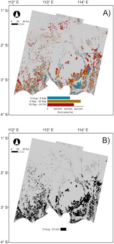
Figure 4 displays the burnt area maps when (i) scars from just pre-fire and post-fire season images
adding the detections from the three mapping periods significantly under-estimates burnt area, in this case
and (ii) using a pair of pre-fire and post-fire season giving 37% less than when adding detections from the
images. When combining the maps from the three dis- three periods.
tinct periods, some areas were mapped as burnt in
more than one period, with these contributing 5.3. Comparison with existing maps of burnt area
approximately 29% to the overall burnt area. Of these, Figure 5 shows the comparison at 5 km scale between
the vast majority (88%) were mapped as burnt in two the burnt area proportion obtained from this study
6Environ. Res. Lett. 15 (2020) 054008
Figure 4. Maps of burnt areas from applying the fitted Random Forests model to Sentinel-1A Interferometric Wide swath data. (A) Adding
detections from the three selected periods; (B) detections using a pair of pre-fire (13 August 2015) and post-fire (24 October) season images.
and those produced by the MCD64A1 global monthly season (13 August–24 October, figure 5(D)) the esti-
burnt area product (Giglio et al 2018) and the mates of burnt area proportion from the MCD64A1
Lohberger et al (2018) regional study. product is on average 34% of those from this study.
The burnt area proportion obtained in this study is Much better agreement is observed between our
consistently much higher than from the MCD64A1 estimate of burnt area proportion during the fire sea-
product. In the first period (13 August–6 September, son and that from Lohberger et al (2018) (figure 5(E)).
figure 5(A)) the estimates of burnt area proportion The regression line has gradient 0.80 (R2=0.82) over
from the MCD64A1 product are on average 51% of the 5 km systematic grid. However, when compared
those obtained from this study. This value decreases to with our overall estimate from adding the detections
28% and 14% in the second (6–30 September, from the three periods (5 km grid=∼1.5 Mha), the
figure 5(B)) and third (30 September–24 October, overall burnt area from Lohberger et al (2018) is much
figure 5(C)) periods, respectively. During the fire smaller (5 km grid=∼1.0 Mha).
7Environ. Res. Lett. 15 (2020) 054008
Figure 5. Density scatterplots comparing burnt area proportion at 5 km scale obtained from this study with the MCD64A1 global
monthly burnt area product (Giglio et al 2018) and the Lohberger et al (2018) regional study. This study versus MCD64A1: (A) 13
August–6 September; (B) 6–30 September; (C) 30 September–24 October; (D) fire season: 13 August–24 October; (E) this study versus
Lohberger et al (2018). The solid lines represent the linear fits between the sets of estimates, with slope: (A) 0.512, (B) 0.277, (C) 0.143,
(D) 0.338, (E) 0.798. The dashed lines represent perfect agreement. Colour intensity is proportional to the number of observations.
6. Discussion machine learning methods to extract this informa-
tion is not straightforward since it involves decisions
The analysis in this paper makes clear that Sentinel-1 about the degree of confidence one has that a
provides a powerful tool for mapping fire scars, fire has occurred and the level of commission error
and can yield important information about fire (or false detections) that is acceptable, as we now
dynamics in the landscape. Also clear is that using discuss.
8Environ. Res. Lett. 15 (2020) 054008
6.1. Algorithmic and data issues affecting (https://globalforestwatch.org) gives access to the loca-
discrimination of burnt areas with Sentinel-1 data tion of forest concessions (including oil palm). For
The empirical basis for detecting burnt area from S1-A Indonesia, these data are provided by the Ministry of
data is clear from figure 2, which shows that both VH Forestry. It may also be possible to extract geometrical
and VV intensity tend to decrease after a fire. At information from the detections in order to recognise
C-band, the VH backscatter from vegetated areas the regular shapes expected under forest management,
mainly arises from volume scattering from leaves and but this would require a substantial amount of develop-
small branches, so tends to decrease when the canopy ment and testing.
is lost due to fire. For VV the situation is more Although errors due to clearcuts, for example, are
complicated, with backscatter mainly coming from inevitable under the methodology used, the primary
canopy elements when the canopy is dense, but control on the structure of the errors is the trade-off
changing to surface and double bounce scattering after between omission and commission errors (figure 3)
canopy loss by fire, especially when this allows which involves decisions that are mostly qualitative
penetration to the ground. Hence the observed reduc- and depend on the classification problem (Freeman
tion in VV backscatter cannot be predicted, and in and Moisen 2008). However, by adding information
some circumstances, fire scars may be brighter at VV or refining the decision rules, it may be possible to
than the surrounding intact forest, particularly if the reduce the commission errors, allowing higher detec-
soil is wet in these areas (Kasischke et al 1994). tion rates to be achieved. For example, information on
We identified several factors that might explain the forest concessions could provide ancillary data that
difference between the overall burnt area estimated would allow a substantial proportion of commission
from adding detections from three periods and when errors to be eliminated. Furthermore, if we were to
using a pair of pre-fire and post-fire season images constrain the detected burnt areas to occur in patches
(figures 4(A) and (B)): greater than a minimum area, then a substantial
component of these areas could be discarded by filter-
(a) The backscatter signal of a fire scar may fade ing processes.
quickly with time and therefore the scar may not Extending this approach to S-1 data at regional or
be detected when only a pair of pre-fire and post- global scales is highly desirable but would involve pro-
fire season images is used. We can point to cessing and storing data volumes many orders of mag-
anecdotal evidence of the fire scar signal fading nitude greater than those from optical sensors
with time, but do not have a precise estimate of currently used to estimate the global spatial distribu-
how much of the difference might be due to this tion of burnt areas. It would also require generating a
effect, which was mostly observed over areas regional- or global-scale dataset of reference observa-
mapped as burnt during the first period (13 tions of unburnt and burnt locations, similar to the
August–6 September), therefore allowing the approach followed by Friedl et al (2010) when devel-
vegetation to recover before the end of the fire oping their algorithm to map land cover types globally
season. at annual time steps using MODIS data (MCD12Q1).
(b) The impact of soil moisture, mainly due to
changing environmental conditions (rainfall 6.2. Causes of mismatch with other maps of
burnt area
events). This is more relevant to burnt area
Figures 3(A)–(D) shows that the estimates of burnt
detection if the algorithm is choosing VV back-
area by 5 km cell obtained from our study are almost
scatter as a predictor.
always higher than those from MODIS (MCD64A1),
(c) The two maps have errors (see validation in and in all periods we observe many cells in which
table 2) and part of the mismatch will be due to Sentinel sees a significant proportion as burnt while
the omission and commission errors in both the MODIS data shows almost no burn. The MODIS
approaches. product is based on optical sensors, so is hindered by
smoke and cloud cover, which in this region and
A known source of error in the methodology season is likely to be very high (table S2, supplementary
adopted here is that some changes in the landscape, information). Daily fractional cloud cover derived
especially clearcutting of forest, will produce back- from the Terra sensor (the MOD06_L2 product)
scatter changes similar to fire and will produce detec- (Platnick et al 2015) was available at a spatial resolution
tions falsely ascribed to fire. The overall magnitude of ∼5 km and covered the 13 August–24 October 2015
of the area affected by such non-fire changes that period analysed in this study. This was averaged by
are mapped as burnt is unknown, but the extent of mapping period over areas detected as burnt in this
such false detections could be estimated if data study. A considerable disagreement between the burnt
about the location of forest concessions and their man- area estimates from this study and MODIS occurred
agement plans were available. The World Resources during those periods of higher fractional cloud cover,
Institute (WRI) Global Forest Watch (GFW) platform which had values 46%, 61% and 67% in the periods
9Environ. Res. Lett. 15 (2020) 054008
13 August–6 September, 6 September–30 September Data availability statement
and 30 September–24 October, respectively. The clear
implication is that the MODIS estimates are severely The data that support the findings of this study are
affected by cloud cover (as one would expect), result- available upon request from the authors.
ing in underestimation of burnt areas and hence GHG
emissions in this region.
ORCID iDs
The estimates of burnt area from Lohberger et al
(2018) were obtained using a set of S-1A IW scenes
Joao M B Carreiras https://orcid.org/0000-0003-
acquired before and after the 2015 fire season (20 June
2737-9420
and 24 October respectively) covering Kalimantan,
Shaun Quegan https://orcid.org/0000-0003-
Sumatra and West Papua. However, we show that this
4452-4829
is likely to have missed a significant proportion of
Kevin Tansey https://orcid.org/0000-0002-
burnt area. There is much better agreement with the
9116-8081
estimates from Lohberger et al (2018) (figure 5(E))
Susan Page https://orcid.org/0000-0002-
than with those from MODIS data (figures 5(A)–(D))
3392-9241
but our study clearly demonstrates that not using
multiple S-1A IW acquisitions during the fire season
resulted in a decreased detection of burnt areas of References
approximately 33%: 1.5 Mha in our study against Breiman L 2001 Random forests Mach. Learn. 45 5–32
1.0 Mha in Lohberger et al (2018). Butler D 2014 Earth observation enters next phase Nature 508 160–1
The constellation of S-1A and S-1B IW acquisi- Chuvieco E, Yue C, Heil A, Mouillot F, Alonso-Canas I, Padilla M,
Pereira J M, Oom D and Tansey K 2016 A new global burned
tions will provide an unprecedented, unique capability
area product for climate assessment of fire impacts Glob. Ecol.
to observe all landmasses every 12 d at ∼10 m spatial Biogeogr. 25 619–29
resolution without having to consider issues related to De Zan F and Guarnieri A M 2006 TOPSAR: terrain observation by
cloud cover. Giglio et al (2013) observe that persistent progressive scans IEEE Trans. Geosci. Remote Sens. 44
2352–60
cloud cover is a severe obstacle to detecting active fires
Fortier J, Rogan J, Woodcock C E and Runfola D M 2011 Utilizing
and fire scars and that this could lead to systematic temporally invariant calibration sites to classify multiple dates
underestimation of burnt area in areas with continual and types of satellite imagery Photogramm. Eng. Remote Sens.
cloud cover. This was also recognised by van der Werf 77 181–9
Freeman E A and Moisen G G 2008 A comparison of the
et al (2010) as one of the most significant uncertainties
performance of threshold criteria for binary classification in
when estimating global fire emissions from burnt area terms of predicted prevalence and kappa Ecol. Modell. 217
products in tropical regions. Huijnen et al (2016) esti- 48–58
mated the carbon emissions from the Indonesian fires Friedl M A, Sulla-Menashe D, Tan B, Schneider A, Ramankutty N,
Sibley A and Huang X M 2010 MODIS collection 5 global
in 2015 using estimates of the fire radiative power
land cover: algorithm refinements and characterization of
(FRP) provided by the MODIS sensors onboard Terra new datasets Remote Sens. Environ. 114 168–82
and Aqua. They note that this system could under- Giglio L, Boschetti L, Roy D P, Humber M L and Justice C O 2018
estimate active fire detections (and hence the corresp- The collection 6 MODIS burned area mapping algorithm and
product Remote Sens. Environ. 217 72–85
onding FRP estimates) because of persistent cloud
Giglio L, Justice C, Boschetti L and Roy D 2015 MCD64A1 MODIS/
cover and smoke over currently burning areas. Terra+Aqua Burned Area Monthly L3 Global 500 m SIN
Grid V006 [Data set]. NASA EOSDIS Land Processes
DAACMCD64A1 MODIS/Terra+Aqua Burned Area
Acknowledgments Monthly L3 Global 500m SIN Grid V006 [Data set]. NASA
EOSDIS Land Processes DAAC (Sioux Falls, SD, USA)
The re-projected monthly GeoTIFF version of the (https://doi.org/10.5067/MODIS/MCD64A1.006)
Giglio L, Loboda T, Roy D P, Quayle B and Justice C O 2009 An
MODIS MCD64A1 burnt area product was made active-fire based burned area mapping algorithm for the
available by the University of Maryland. The daily MODIS sensor Remote Sens. Environ. 113 408–20
MODIS MCD14ML active fire product was produced Giglio L, Randerson J T and van der Werf G R 2013 Analysis of daily,
by the University of Maryland and provided by NASA monthly, and annual burned area using the fourth-
generation global fire emissions database (GFED4)
FIRMS operated by NASA/GSFC/ESDIS with fund- J. Geophys. Res.-Biogeosci. 118 317–28
ing provided by NASA/HQ. The daily Terra MODIS Gregoire J M, Tansey K and Silva J M N 2003 The GBA2000
MOD06_L2 fractional cloud cover product was down- initiative: developing a global burnt area database from
loaded from NASA’s Level-1 and Atmosphere Archive SPOT-VEGETATION imagery Int. J. Remote Sens. 24
1369–76
& Distribution System (LAADS) Distributed Active Hansen M C et al 2013 High-resolution global maps of 21st-century
Archive Center (DAAC). We acknowledge and thank forest cover change Science 342 850–3
ESA CCI Fire for providing access to a burnt area map Harris N L, Brown S, Hagen S C, Saatchi S S, Petrova S, Salas W,
of Kalimantan. JMBC and SQ were supported by the Hansen M C, Potapov P V and Lotsch A 2012 Baseline map of
carbon emissions from deforestation in tropical regions
Natural Environment Research Council (Agreement Science 336 1573–6
PR140015 between NERC and the National Centre for Huijnen V, Wooster M J, Kaiser J W, Gaveau D L A, Flemming J,
Earth Observation). Parrington M, Inness A, Murdiyarso D, Main B and
10Environ. Res. Lett. 15 (2020) 054008
Van Weele M 2016 Fire carbon emissions over maritime emissions from small fires J. Geophys. Res.-Biogeosci. 117
southeast Asia in 2015 largest since 1997 Sci. Rep. 6 26886 G04012
Kasischke E S, Bourgeauchavez L L and French N H F 1994 Reiche J et al 2016 Combining satellite data for better tropical forest
Observations of variations in ERS-1 SAR image intensity monitoring Nat. Clim. Change 6 120–2
associated with forest-fires in Alaska IEEE Trans. Geosci. Richards J A 2009 Remote Sensing with Imaging Radar (Heidelberg,
Remote Sens. 32 206–10 New York: Springer)
Lambin E F, Geist H J and Lepers E 2003 Dynamics of land-use and Schroeder W, Csiszar I and Morisette J 2008 Quantifying the impact
land-cover change in tropical regions Annu. Rev. Environ. of cloud obscuration on remote sensing of active fires in the
Resour. 28 205–41 Brazilian Amazon Remote Sens. Environ. 112 456–70
Lohberger S, Stängel M, Atwood E C and Siegert F 2018 Spatial Sedano F, Kempeneers P, Miguel J S, Strobl P and Vogt P 2013
evaluation of Indonesia’s 2015 fire-affected area and Towards a pan-European burnt scar mapping methodology
estimated carbon emissions using Sentinel-1 Glob. Change based on single date medium resolution optical remote
Biol. 24 644–54 sensing data Int. J. Appl. Earth Obs. Geoinf. 20 52–9
Menges C H, Bartolo R E, Bell D and Hill G J E 2004 The effect of Siegert F and Hoffmann A A 2000 The 1998 forest fires in East
savanna fires on SAR backscatter in northern Australia Int. J. Kalimantan (Indonesia): a quantitative evaluation using high
Remote Sens. 25 4857–71 resolution, multitemporal ERS-2 SAR images and NOAA-
Miettinen J, Langner A and Siegert F 2007 Burnt area estimation for AVHRR hotspot data Remote Sens. Environ. 72 64–77
the year 2005 in Borneo using multi-resolution satellite Silva J M N, Sa A C L and Pereira J M C 2005 Comparison of burned
imagery Int. J. Wildland Fire 16 45–53 area estimates derived from SPOT-VEGETATION and
Miettinen J, Shi C and Liew S C 2016 Land cover distribution in the Landsat ETM plus data in Africa: influence of spatial pattern
peatlands of Peninsular Malaysia, Sumatra and Borneo in and vegetation type Remote Sens. Environ. 96 188–201
2015 with changes since 1990 Glob. Ecol. Conservation 6 Simon M, Plummer S, Fierens F, Hoelzemann J J and Arino O 2004
67–78 Burnt area detection at global scale using ATSR-2: the
Moreira A, Prats-Iraola P, Younis M, Krieger G, Hajnsek I and GLOBSCAR products and their qualification J. Geophys. Res.-
Papathanassiou K P 2013 A tutorial on synthetic aperture Atmos. 109 D14S02
radar IEEE Geosci. Remote Sens. Mag. 1 6–43 Torres R et al 2012 GMES Sentinel-1 mission Remote Sens. Environ.
Olofsson P, Foody G M, Herold M, Stehman S V, 120 9–24
Woodcock C E and Wulder M A 2014 Good practices for Tyukavina A, Baccini A, Hansen M C, Potapov P V, Stehman S V,
estimating area and assessing accuracy of land change Remote Houghton R A, Krylov A M, Turubanova S and Goetz S J 2015
Sens. Environ. 148 42–57 Aboveground carbon loss in natural and managed tropical
Page S E, Siegert F, Rieley J O, Boehm H D V, Jaya A and Limin S forests from 2000 to 2012 Environ. Res. Lett. 10 074002
2002 The amount of carbon released from peat and forest van der Werf G R, Randerson J T, Giglio L, Collatz G J, Mu M,
fires in Indonesia during 1997 Nature 420 61–5 Kasibhatla P S, Morton D C, Defries R S, Jin Y and
Platnick S, Ackerman S A, King M D, Meyer K, Menzel W P, Van Leeuwen T T 2010 Global fire emissions and the
Holz R E, Baum B A and Yang P 2015 MODIS Atmosphere L2 contribution of deforestation, savanna, forest, agricultural,
Cloud Product (06_L2), NASA MODIS Adaptive Processing and peat fires (1997–2009) Atmos. Chem. Phys. 10 11707–35
System (Greenbelt, MD: Goddard Space Flight Center) Woodhouse I H 2006 Introduction to Microwave Remote Sensing
(https://doi.org/10.5067/MODIS/MOD06_L2.006) (Boca Raton, FL: Taylor and Francis)
Quegan S and Yu J J 2001 Filtering of multichannel SAR images Wooster M J, Xu W and Nightingale T 2012 Sentinel-3 SLSTR active
IEEE Trans. Geosci. Remote Sens. 39 2373–9 fire detection and FRP product: pre-launch algorithm
Randerson J T, Chen Y, van der Werf G R, Rogers B M and development and performance evaluation using MODIS and
Morton D C 2012 Global burned area and biomass burning ASTER datasets Remote Sens. Environ. 120 236–54
11You can also read