Sliced Optimal Transport Sampling - Applied Geometry Lab
←
→
Page content transcription
If your browser does not render page correctly, please read the page content below
Sliced Optimal Transport Sampling
LOIS PAULIN, Univ Lyon, CNRS
NICOLAS BONNEEL, Univ Lyon, CNRS
DAVID COEURJOLLY, Univ Lyon, CNRS
JEAN-CLAUDE IEHL, Univ Lyon, CNRS
ANTOINE WEBANCK, Univ Lyon, CNRS
MATHIEU DESBRUN, ShanghaiTech/Caltech
VICTOR OSTROMOUKHOV, Univ Lyon, CNRS

                              Ref.                           White noise                      Dart throwing              Sobol                          Ours

Fig. 1. Sliced Optimal Transport Sampling. Global illumination of a scene (top left, San Miguel) requires integrating radiance over a high-dimensional
space of light paths. The projective variant of our sliced optimal transport (SOT) sampling technique, leveraging the particular nature of integral evaluation in
rendering and further combined with a micro-Cranley-Patterson rotation per pixel, outperforms standard Monte Carlo and Quasi-Monte Carlo techniques,
exhibiting less noise and no structured artifact (top right, 32spp) while offering a better spatial distribution of error (bottom right, errors from blue (small)
to red (large)). Moreover, our projective SOT sampling produces better convergence of the mean absolute error for the central 7×7 zone of the highlighted
reference window as a function of the number of samples per pixel (from 4spp to 4096spp, bottom-left graph) in the case of indirect lighting with one bounce.

In this paper, we introduce a numerical technique to generate sample dis-                        mapping to arbitrary dimensions) to offer fast SOT sampling over d -cubes.
tributions in arbitrary dimension for improved accuracy of Monte Carlo                           We provide ample numerical evidence of the improvement in Monte Carlo
integration. We point out that optimal transport offers theoretical bounds                       integration accuracy that SOT sampling brings compared to existing QMC
on Monte Carlo integration error, and that the recently-introduced numeri-                       techniques, and derive a projective variant for rendering which rivals, and
cal framework of sliced optimal transport (SOT) allows us to formulate a                         at times outperforms, current sampling strategies using low-discrepancy
novel and efficient approach to generating well-distributed high-dimensional                     sequences or optimized samples.
pointsets. The resulting sliced optimal transport sampling, solely involving                     CCS Concepts: • Computing methodologies → Computer graphics.
repeated 1D solves, is particularly simple and efficient for the common case                     Additional Key Words and Phrases: multidimensional sampling, optimal
of a uniform density over a d -dimensional ball. We also construct a volume-
                                                                                                 transport, Radon transform, Monte Carlo integration, point distributions
preserving map from a d -ball to a d -cube (generalizing the Shirley-Chiu
                                                                                                 ACM Reference Format:
                                                                                                 Lois Paulin, Nicolas Bonneel, David Coeurjolly, Jean-Claude Iehl, Antoine
Authors’ addresses: Lois Paulin, Nicolas Boneel, David Coeurjolly, Jean-Claude Iehl,
                                                                                                 Webanck, Mathieu Desbrun, and Victor Ostromoukhov. 2020. Sliced Optimal
Antoine Webanck, Victor Ostromoukhov: CNRS/LIRIS, Lyon, France; Mathieu Des-
brun: California Institute of Technology, Pasadena, CA, USA, on sabbatical at SIST in            Transport Sampling. ACM Trans. Graph. 39, 4, Article 1 (July 2020), 17 pages.
ShanghaiTech University, Shanghai, China.                                                        https://doi.org/10.1145/3386569.3392395
Permission to make digital or hard copies of all or part of this work for personal or
classroom use is granted without fee provided that copies are not made or distributed
                                                                                                 1   INTRODUCTION
for profit or commercial advantage and that copies bear this notice and the full citation           The need to evaluate integrals of high-dimensional signals arises
on the first page. Copyrights for components of this work owned by others than ACM
must be honored. Abstracting with credit is permitted. To copy otherwise, or republish,          in a number of applications such as finance or machine learning.
to post on servers or to redistribute to lists, requires prior specific permission and/or a      It is particularly crucial in global illumination where the radiance
fee. Request permissions from permissions@acm.org.                                               through a pixel must be integrated across the multidimensional
© 2020 Association for Computing Machinery.
0730-0301/2020/7-ART1 $15.00                                                                     space of possible light transport paths. Monte Carlo integration,
https://doi.org/10.1145/3386569.3392395                                                          which approximates an integral through averaging the values of

                                                                                                            ACM Trans. Graph., Vol. 39, No. 4, Article 1. Publication date: July 2020.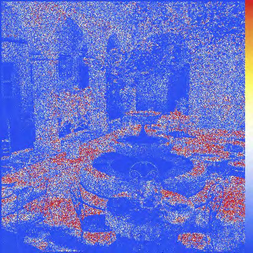
1:2 •   Paulin, et al.

its integrand evaluated at n discrete locations within the integra-          cube [0, 1]d is bounded by the product of two independent factors:
tion domain, is often the only practical technique to handle this                                     n
                                                                                                   1Õ
                                                                                     ∫
challenging numerical task.                                                              f (x)dx −       f (x i ) ≤ D({x 1, ..., x n }). VarHK f , (1)
                                                                                                   n i=1
   While the original Monte Carlo (MC) technique relies on random
sample locations, the resulting approximation error is often greatly         where D(.) is the so-called discrepancy of a point distribution mea-
affected by sample clumping: intuitively, the amount of information          suring its spatial uniformity, while VarHK f measures the variation
gathered by each sample on the integrand should be maximized, so             of the function f in the sense of Hardy and Krause (a multidimen-
clumped samples are wasteful. Since the simple choice of regular             sional extension of total variation), see [Hlavka 1961]. Evaluating
grid distributions (possibly jittered to avoid aliasing) is ill-suited       this discrepancy is particularly costly as it requires finding the
to the case of high dimensions, several efforts to define the notion         worst-case density deviation from a uniform pointset over arbitrary
of “well-distributed” sampling followed. Guided by a known bound             convex regions. As a result, simpler notions of discrepancy (like the
on integration error depending on a measure of spatial uniformity            star discrepancy D ∗ involving only boxes with a corner at 0, the
of the samples called discrepancy, quasi-Monte Carlo (QMC) meth-             extreme discrepancy, or the L 2 discrepancy) have been proposed,
ods proposed the use of specifically-crafted deterministic sample            still offering valid — yet less tight — error bounds. Finally, note
locations, typically generated via low-discrepancy sequences. This           that Eq. (1), and thus the notion of discrepancy, is only useful in
family of approaches is currently the cornerstone of most rendering          bounding the error for functions of finite Hardy-Krause variation; in
algorithms as it greatly improves the integration accuracy for a fixed       particular, MC integration of discontinuous multivariate functions
number of samples. More recently, spectral statistics of the spatial         may result in large errors, while typical functions may have actual
distribution of samples have also been proven key to reducing the            errors far lower than the provided upper bound. When no a-priori
approximation error, suggesting that carefully optimized sampling            knowledge is available on the function f , the integration error be-
locations can further improve upon low-discrepancy sequences.                ing bounded by discrepancy implies that using sample distributions
Since optimizing sample distributions over high dimensional do-              with low discrepancy is a reliable way to bound the expected MC
mains is computationally challenging, variational approaches to              error. Fortunately, there exists by now a series of sequences (de-
sampling (where samples are optimized to minimize a select mea-              terministic enumeration of samples) which offer low discrepancy
sure of uniformity) have only been offered in low dimensions so far.         by construction, the most popular ones being Sobol, Halton, Faure,
Yet, none specifically targets the reduction of Monte Carlo integra-         van der Corput, and Niederreiter sequences (see recent surveys
tion error, focusing instead of stippling or halftoning applications.        in [Lemieux 2009; Dick and Pillichshammer 2010; Keller 2013]). The
   In this paper, we argue for the design of high-dimensional sam-           term quasi-Monte Carlo (QMC) refers to methods based on these
pling via optimal transport, and provide an efficient and practical          low-discrepancy sequences for MC integration. As evidenced by
sample distribution optimization method in arbitrary dimensions              their wide use in modern rendering engines such as PBRT [Pharr
through sliced optimal transport, solely involving repeated 1D solves.       et al. 2016] or Mitsuba [Jakob 2013], QMC approaches are considered
We provide ample numerical evidence of improved accuracy of                  state-of-the art for error minimization in radiance estimation.
Monte Carlo integrations, and derive a projective variant which                 Variational blue noise distributions. Another notion of equidistri-
rivals, and at times outperforms, current rendering strategies.              bution of point samples was introduced by Robert Ulichney [Ulich-
                                                                             ney 1987] in terms of spectral content: a pointset is said to exhibit
1.1     Background                                                           “blue noise” characteristics if its isotropic power spectrum has no
   We begin with a brief review of previous works on the generation          low-frequency components, has a peak at a characteristic frequency
of sample distributions (i.e., pointsets) for integration purposes.          (representing the inverse of the mean distance between points), and
                                                                             is flat (white noise) at high frequencies. Recent work theoretically
   Poisson disk sampling. A common approach to generating well-
                                                                             confirmed that having no low frequency content in the spectrum of
spread point distributions is through Poisson disk sampling, which
                                                                             a sample distributions ensures better Monte Carlo integration [Du-
guarantees that two points are separated by at least a given min-
                                                                             rand 2011; Subr and Kautz 2013; Pilleboue et al. 2015; Öztireli 2016;
imum distance. While fast to generate using dart throwing tech-
                                                                             Singh and Jarosz 2017; Singh et al. 2019], explaining a posteriori
niques [Bridson 2007], Poisson disk samples suffer from an inherent
                                                                             why a few popular sampling schemes such as Poisson-disk sampling
white noise component [Torquato et al. 2006] that gravely weakens
                                                                             exhibit an asymptotic behavior no better than using random points.
its relevance to integration purposes in high dimension.
                                                                             While blue noise distributions in graphics were leveraged early on to
   Low-discrepancy distributions. While a multitude of quadrature            remove the harmful aliasing artifacts of regular sampling [Dippé and
methods for numerical integration exist in two or three dimensions,          Wold 1985; Cook 1986; Mitchell 1987, 1991], they regained consider-
Monte Carlo (MC) integration has remained the method of choice for           able attention within the computer graphics community recently:
the evaluation of high-dimensional integrals: its stochastic nature          their spatial distribution in 2D visually offers a good balance be-
offers an expected accuracy independent of the dimensionality of             tween ordered and disordered distributions [Georgiev and Fajardo
the domain of integration. However, this same randomness in the              2016; Heitz and Belcour 2019; Heitz et al. 2019], making them partic-
locations of samples often leads to large approximation errors, unless       ularly well suited for stippling and halftoning. Consequently, many
many samples are employed. A better understanding of this issue              variational approaches for generating blue noise pointsets through
can be gained by considering the Koksma-Hlawka inequality, which             optimization of sample positions have been proposed over the last
states that the accuracy of MC integration over a d-dimensional unit         decade [Ostromoukhov et al. 2004; Kopf et al. 2006; Lagae and Dutré

ACM Trans. Graph., Vol. 39, No. 4, Article 1. Publication date: July 2020.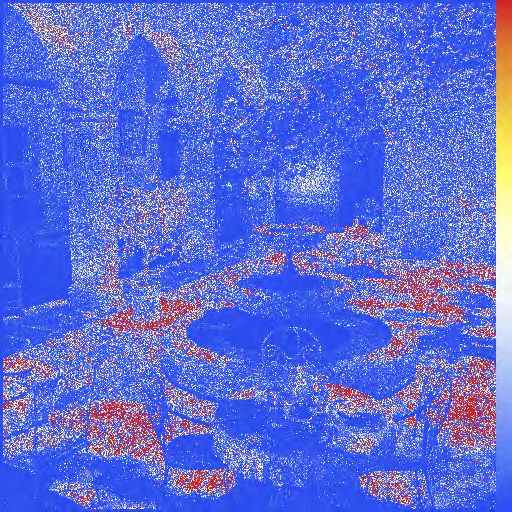
Sliced Optimal Transport Sampling • 1:3

2006; Wei 2010; Fattal 2011; Zhou et al. 2012; Heck et al. 2013]. Most     2 RELEVANCE OF OPTIMAL TRANSPORT TO SAMPLING
germane to our work is the fact that a few variational blue noise            Optimal transport (OT) is a theoretical framework useful in a
sampling techniques define their measure of uniformity through             variety of fields, from economics for resource allocation to math-
optimal transport [Balzer et al. 2009; De Goes et al. 2012; Qin et al.     ematical physics for hydrodynamics. In its most general form, it
2017]; regrettably, their scalability in 2D and 3D does not extend to      defines a formal notion of distance between generalized probability
arbitrary dimensions, and no discussions on approximation errors           density functions by evaluating an optimal transport plans between
when used for Monte Carlo integration were provided.                       them [Villani 2009]: intuitively, if each density is viewed as a given
   Projective sampling. Recent works [Kulla et al. 2018; Christensen       amount of sand piled up in space, this metric is the minimum labor
et al. 2018a; Jarosz et al. 2019] proposed to improve uniformity of        needed to move one pile into the other. In our sampling context,
sampling distributions in low and high dimensions by starting from         though, the simpler, but more specific notion of semi-discrete op-
good 2D configurations that they then lift to higher dimensions.           timal transport is most relevant to our goals: it provides a simple
In sharp contrast, [Reinert et al. 2016] introduced an approach to         approximation bound for Monte Carlo integration, which we will
optimize spatial positions of multidimensional pointsets while pre-        exploit for sampling generation in the remainder of this paper.
serving spectral properties of lower-dimensional projections. Our
approach will be able to accommodate this projective sampling              2.1   Distance of samples to spatial density
idea (without suffering from the combinatorial explosion in high              Optimal transport also allows to quantify how well a pointset
dimensions), which we will then leverage for rendering purposes.           matches a given density function: as points in arbitrary dimensions
                                                                           can be thought of as Dirac masses, OT provides a measure of how
1.2   Contributions                                                        much the points need to spread out (i.e., transport their mass across
   Designing pointsets in arbitrary dimensions to ensure good accu-        space) to match the density function. This particular case is often
racy in MC integration remains a difficult goal. The sparsity of theo-     referred to semi-discrete optimal transport, and when applied to a
retical foundations is a first issue: one can only leverage knowledge      uniform density function, it defines an intuitive notion of “equidis-
on either the role of discrepancy or partial spectral properties, which    tribution” for a pointset, very different from discrepancy.
limits the number of approaches that one can design to construct              More precisely, the semi-discrete optimal transport distance be-
good sample distributions. A second issue is the need for sampling         tween a spatial density φ within a domain Ω ⊂ Rd and a set of n
in arbitrary dimensions. While low-discrepancy sequences are nat-          sample points X = {xj ∈ Ω}j=1..n can be mathematically formulated
urally able to handle a high dimensional domain, their discrepancy         as finding a spatial assignment π: Ω → {1,...,n} of every point x of Ω
in this case might not be smaller than for a random set for practical      to a sample xπ (x) that minimizes what is known as the p-Wasserstein
values of the number of samples n [Lemieux 2009]; moreover, their          distance Wp (X, φ), defined as:
periodic structure is known to generate visual artifacts in rendering                                  ∫                           1/p
applications [Pharr et al. 2016].                                                    Wp (X, φ) B min        ∥x − xπ (x ) ∥p φ(x)dx       ,     (2)
                                                                                                       π     Ω
   In this paper, we point out that optimal transport offers theoret-
ical grounds to bound MC integration that are similar, yet differ-         under the constraint    that each sample is considered to have the
                                                                           same mass, i.e., π −1 (j) φ(x)dx = n1 ∀j ∈ {1,...,n}. In the case p = 2,
                                                                                             ∫
ent from the discrepancy-based bound from Eq. (1), and that the
recently-introduced numerical framework of sliced optimal trans-           a constrained optimization of the distance W2 (X, φ) to compute a
port [Pitié et al. 2005; Rabin et al. 2011; Bonneel et al. 2015; Bonneel   pointset X best matching a spatial density φ is known to be effi-
and Coeurjolly 2019] allows us to formulate a novel and efficient          ciently achieved via power diagrams [Aurenhammer et al. 1998].
approach to generating well-distributed high-dimensional pointsets.        This is precisely the approach adopted by a number of recent works
While the resulting sliced optimal transport (SOT) sampling can            in graphics to compute “blue noise” pointsets sampling a given
handle arbitrary densities over arbitrary domains through the sliced       continuous density [Mérigot 2011; De Goes et al. 2012; Lévy 2015;
Fourier theorem, the archetypical case of a uniform density over a         Qin et al. 2017; Nader and Guennebaud 2018] through gradient
d-dimensional ball is particularly simple and efficient computation-       or Newton descent; yet none of these techniques are practical in
ally. We further introduce a bi-Lipschitz volume-preserving map            higher dimensions. Optimal transport was also used in [Rowland
from the d-ball to the d-cube (generalizing the original Shirley-Chiu      et al. 2018] to couple subsets of multidimensional pointsets.
area-preserving disk-to-square mapping [Shirley and Chiu 1997]) to         2.2   Error bounds for Monte Carlo integration
handle the d-cube case efficiently as well. We then present a wide
                                                                              The Rubinstein-Kantorovich theorem [Kantorovich 1948; Kan-
array of numerical tests for various dimensions d to demonstrate
                                                                           torovich and Rubinstein 1958] states through a duality argument
the excellent approximation accuracy of our optimized sample dis-
                                                                           that the Wasserstein distance W1 (µ, ν ) for two densities µ and ν can
tributions. Finally, we show that our technique can exploit specific
                                                                           in fact be seen as an upper bound for finite Lipschitz functions of
properties of the integrands to further decrease approximation error:
                                                                           the difference of their integrals over these
                                                                                                                    ∫ two measures:
building upon the idea of projective blue noise [Reinert et al. 2016]
                                                                                                               1
for rendering, we can specialize SOT sampling to generate samples                     W1 (µ, ν ) = sup                   f (x) d(µ − ν ),      (3)
with both near equidistribution in the high-dimensional space and                                 f : Rd →R Lip(f ) R
                                                                                                                       d

near equidistribution of their projections onto select linear sub-         where Lip(f ) represents the Lipschitz constant of function f . While
spaces. Rendering examples demonstrate clear improvements over             this equivalent definition of the optimal transport distance is rarely
standard QMC methods used in rendering engines, see Fig. 1.                used in graphics (with the notable exception of [Mullen et al. 2011]),

                                                                                     ACM Trans. Graph., Vol. 39, No. 4, Article 1. Publication date: July 2020.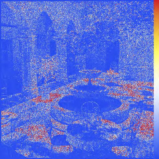
1:4 •   Paulin, et al.

it is especially interesting in our semi-discrete setting: it allows us      3     SLICED OPTIMAL TRANSPORT SAMPLING
to derive a tight bound of the MC integration error for Lipschitz               This section details the main theoretical and practical aspects of
continuous functions. In particular, using a uniform density dx/|Ω|          our algorithm. We first review the general approach, before showing
over the d-dimensional     domain Ω, we deduce from Eq. (3) that for a       how to efficiently adapt it for the uniform sampling of a d-ball and
sample set X = x 1, ..., x n , one has for any Lipschitz function f :

                                                                             a d-cube. We also extend our approach to provide projective SOT
                              n
                           1Õ                                                sampling for rendering purposes.
            ∫
                f (x) dx −       f (x i ) ≤ Lip(f ) .W1 (X, 1Ω ),   (4)
                           n i=1
                                                                             3.1    Sliced optimal transport formulation
where 1Ω denotes the constant density 1/|Ω|. This derived bound has
                                                                                The core idea of our approach is to cast the problem of sampling
a very similar form as the Koksma-Hlawka inequality from Eq. (1):
                                                                             a distribution in term of the minimization of a sliced optimal trans-
it also offers an error bound written as the product of two separate
                                                                             port distance [Rabin et al. 2011; Bonneel et al. 2015], for which
factors, one only dependent on the function being integrated, and
                                                                             repeated 1D transports can be used to spread samples efficiently in
one purely based on a measure of spatial uniformity — which is no
                                                                             arbitrary dimensions. To this effect, we define a SOT distance (or
longer the discrepancy, but an optimal transport analog. Note that
                                                                             cost) WSOT (X, φ) between a density
                                                                                                            ∫ φ and a pointset X as:
while the Koksma-Hlawka bound was assuming that the function                                     ∫
                                                                                                                            π (x )
had a finite Hardy-Krause variation, this one now assumes that the                 WSOT (X, φ) =           min   ∥x − x θ ∥ Rθ φ(x) dx dθ , (6)
                                                                                                   Sd −1   π
function is Lipschitz continuous instead. Thus, the OT-based bound                                            R
                                                                             where dx denotes the 1D measure, θ denotes a direction (unit vec-
is technically more restrictive in its assumption of the integrand.                                j
                                                                             tor in Sd−1 ⊂ Rd ), x θ B xj ·θ is the 1D abscissa representing the
However, Lipschitz continuity is a reasonable assumption in many
                                                                             orthogonal projection of sample point xj from X onto the 1D linear
graphics applications; moreover, both functional spaces fail to in-
                                                                             subspace along θ , and Rθ φ is the
                                                                                                             ∫ scalar function defined as
clude basic discontinuous functions, and practical functions may
lead to actual integration errors below both theoretical bounds.                                   Rθ φ(s) B              φ(x) dx .             (7)
                                                                                                                 θ ·x=s
2.3     Computational optimal transport in high dimension                    One recognizes Rθ φ(s) as the Radon transform [Radon 1986] of
                                                                             the density φ, integrating the density φ in the affine subspace or-
   Equipped with the error bound from Eq. (4), one may be tempted
                                                                             thogonal to a “slice” direction θ ∈ Sd−1 at abscissa s. Our sliced
to directly optimize a sample distribution by minimizing its Wasser-
                                                                             optimal transport distance can be understood as an integral over all
stein distance to the uniform density. However, and despite a num-
                                                                             directions θ of the 1D (classical) optimal transport cost W1 between
ber of numerical optimal transport tools recently introduced in
                                                                             the projection of the pointset X along direction θ and the orthog-
graphics [De Goes et al. 2012; Solomon et al. 2014, 2015; Nader and
                                                                             onal projection of the spatial density φ along this same direction:
Guennebaud 2018], dealing with transport optimization in high
                                                                             essentially, we express the fit between a pointset and a density by
dimensions is not computationally tractable directly. Fortunately,
                                                                             the integral of the fit of their 1D projections, see Fig. 2. Instead,
a recent variant of optimal transport offers a practical solution. A
                                                                             previous work considered W2 for sliced distances [Rabin et al. 2011;
modified notion of optimal transort, now called sliced optimal trans-
                                                                             Bonneel et al. 2015]; but the W1 optimization, which provides a
port (SOT [Pitié et al. 2005; Rabin et al. 2011; Bonneel et al. 2015;
                                                                             tighter bound, results in the same 1D assignments, although the
Bonneel and Coeurjolly 2019]), proposes to express the transport
                                                                             optimal assignment is no longer unique.
distance between two densities via an integral of 1D optimal trans-
                                                                                As a consequence, this formulation has a number of advantages
port distances between all 1D projections of these densities. Given
                                                                             that we can leverage for computational purposes. First, reducing
that semi-discrete optimal transport in 1D amounts to a simple sort
                                                                             the distance one (or a few) direction(s) at a time is very efficient as
(for all p-Wasserstein distances Wp , p ≥ 1), the SOT distance WSOT is
                                                                             we shall see next, in sharp contrast to the general optimal transport
amenable to tractable computational evaluations and optimizations
                                                                             problem. Second, once a distribution is optimized with respect to a
even in dimensions well above three through repeated 1D optimiza-
                                                                             direction θ , it cannot have sample alignments along hyper-planes
tions. However, to our knowledge, neither semi-discrete transport
                                                                             orthogonal to θ : this naturally prevents aliasing artifacts and offers
nor the optimal location problem have been previously investigated
                                                                             the opportunity to prevent alignments in specific subspaces as well,
in the sliced optimal transport context. Moreover, the sliced optimal
                                                                             as we will explore in Sec. 3.6. Third, our iterative optimization is
transport distance being bounded by the d-th power of the optimal
                                                                             agnostic to the domain dimensionality.
transport distance W1 [Bonnotte 2013], the bound from Eq. (4) with
sliced optimal transport becomes:                                            3.2    General approach to SOT sampling
                         n
                      1Õ                                                        Our sliced OT approach immediately suggests an algorithmic
        ∫
                                                                  1
           f (x) dx −       f (x i ) ≤ Cd Lip(f ) WSOT (X, 1Ω ) d +1 , (5)
                      n i=1                                                  approach to optimizing a pointset: one can project both the target
where Cd is a constant that depends on the dimension d. Using SOT            density and the pointset onto a series of one-dimensional lines, and
instead of OT is thus akin to using a simplifications of the notion          successively optimize the location of all points along each of these
of discrepancy in QMC approaches: it only relaxes the error bound            directions to improve the one-dimensional fit between projected
on integration errors. We are now ready to introduce the notion of           sample density and projected target density.
sliced optimal transport for sampling by adapting previous work to             Discrete set of directions. In order to discretize Eq. (6), we first
our context of semi-discrete transport discussed above, and derive a         randomly sample K directions {θ i }i=1..K (typically we use K =
novel algorithm for the generation of equidistributed sample points.         64). Generating each direction with a uniform probability over the

ACM Trans. Graph., Vol. 39, No. 4, Article 1. Publication date: July 2020.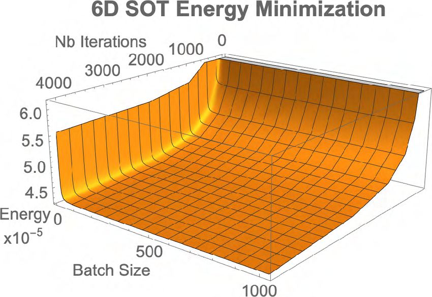
Sliced Optimal Transport Sampling • 1:5
sorts of n projected points per iteration (i.e., O(Kn log n)), as well
as the cost for computing (or precomputing) the Radon transform
in a number of directions. We show next that this last task can be
achieved in constant time for a simple, yet very common case.
3.3 Uniform SOT sampling over d-balls
A key component of our formulation is the (partial) Radon trans-
form Rθ φ of the density φ in a direction θ , and its inverse cumulative
θ distribution function. Numerical tools based on the Fast Fourier
xj Transform and the so-called Fourier slice theorem allow for the effi-
⟨xj , θ ⟩ cient numerical evaluation the Radon transform [Toft and Sørensen
σ (j)−0.5 1996] on discretized domain. However, such numerical approxima-
Cd−1 (θ, )
n tions can become impractical when dealing with very high dimen-
{δδ j } sions unless a closed-form expression of the Fourier transform is
known. Fortunately, the particular, yet common case of a uniform
Fig. 2. Optimal transport via one-dimensional slices. Our approach density on a unit d-ball is particularly simple to evaluate without
adapts a distribution of n samples (green dots) to a spatial density function advanced numerical methods. Indeed, the radial symmetry of the
(here, uniform, in grey) in arbitrary dimension through iterative 1D optimiza-
d-ball implies that the Radon transform does not depend on the
tion of the sliced optimal transport energy between the projected samples
(green circles) onto an arbitrary direction θ and the density projected or-
chosen direction θ . We will hence denote it as Rφ(s) B Rθ φ(s) ∀θ .
thogonally to this direction. The blue curve indicates the Radon transform Additionally, when φ is a uniform density, we can explicitly compute
of the disk-shaped density,and the red dots indicate the directional update the resulting Radon transform in closed form: its cumulative density
δ j of the samples to optimize their distribution along θ . function becomes trivial to evaluate for odd-dimensional spaces,
and requires only little additional effort for even-dimensional spaces.
hypersphere Sd−1 is trivially achieved by first generating d random We prove in App. A that the expression for the function Rφ and its
variables following a normal distribution N (0, 1), and normalizing cumulative density function Cd in dimension d is:
these variables to obtain the components of a unit vector. π d/2 p
Radon transform. We then compute the Radon transform of φ
Rφ(s) =
d 1 − s 2, and (8)
Γ 2 +1
along the directions {θ i }i . The Radon transform defines a new prob-
ability density function Rθ i φ, of which we compute the cumulative (d−1)/2
k d−1
density function Cθ i defined as: x 2k +1
if d is odd,
Í
(−1) 2
2k+1
∫ x k =0 k
Cd (x) = √ (9)
Cθ i (x) B Rθ i φ(s)ds,
π Γ 1+d
1 1−d 3 2
2 Γ 1+ d + 2F 1 2 , 2 , 2 , x x if d is even,
−∞ 2
and its inverse Cθ−1 (x) B inf {t ∈ R : Cθ i (t) > x }. 2
i
Slice optimization. Finally, we relocate the sample point xj to a where Γ(.) is the Gamma function, and 2F 1 (.) is the so-called hyper-
new location xj +δδ j , where the total displacement δ j is geometric function, involving polynomials and trigonometric func-
K
1 Õ tions; see Fig. 3. We further invert the cumulative density function
δj B di,j θ i , numerically using a gradient descent approach to offer an efficient
K i=1
way to evaluate the inverse cumulative density function Cd−1 (x): this
with di,j being the displacement of xj that minimize the 1D sliced
inverse function is tabulated once and for all as a precomputation.
optimal transport along direction θ i . Denoting σ the permutation
of the indices {j}j=1..n such that xσ (j) · θ i j , is a sorted sequence
of increasing values, one computes di,j directly via 5 3D Ball 5 2D Ball
5D Ball 4D Ball
σ (j) − 12 6D Ball
7D Ball
di,j = Cθ−1 . 4 9D Ball 4 8D Ball
i n 11D Ball 10D Ball
Spreading samples according to the Radon transform of the density 3 3
along the set of chosen directions then minimizes W1 along these
directions — thus improving the error bound from Eq. (5). 2 2
Discussion. The implementation of our approach is thus concep- 1 1
tually simple: after initializing the pointset with a scrambled Sobol
sequence [Owen 1998] (which offers, at very low computational -1.0 -0.5 0.5 1.0 -1.0 -0.5 0.5 1.0
cost, a better initial distribution than a random distribution), the it- Fig. 3. Radon for d -balls. The Radon transform of a d-ball is direction-
erative process considering K slices at a time to displace the samples independent, so we display the radial component of the Radon transform
is repeated until convergence or when a fixed maximum number of a ball as the dimension d increases. While the transform is polynomial
of steps is reached. Note that the cost of the algorithm involves K for odd dimensions (left), it involves the hypergeometric 2 F 1 function for
even dimensions (right).
ACM Trans. Graph., Vol. 39, No. 4, Article 1. Publication date: July 2020.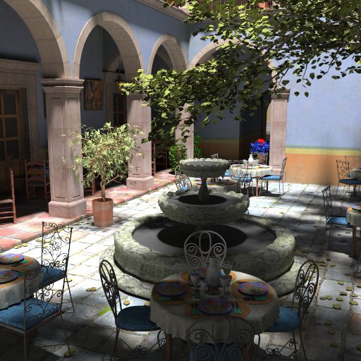
1:6 •     Paulin, et al.

                   y
   B                                                                            Table 1. Ball-to-cube map parameters. Values of γ , ϱ, and τ to compute
                                                                                 the invertible map of Griepentrog et al. [2008] for dimensions d ≤ 10.
               γ                                                                       dim.           γ
                                                                                                       √
                                                                                                                           ϱ                    τ
                                                                                                                                               √ √
   B                                                                                   3           2/ 5                 2/3                   2/ 3
                                                                                         4    0.821353089207943    0.5890486225480863   0.8382695966098716
                                                                                         5    0.7666031370294717   0.5333333333333332   0.8545740127924683
                                                                                         6    0.723424902134195    0.4908738521234051   0.8673491949880967
                           Φtmp                                                          7    0.6881297272460576   0.4571428571428572   0.8776916965664375
   B∆                                                                                    8    0.6585046305043636   0.4295146206079796   0.8862745508336505
Fig. 4. Ball-to-cube map in arbitrary dimension. We illustrate the ball-                 9    0.6331279880529004   0.4063492063492063   0.8935367660649970
                                                                                        10    0.611037644218746    0.3865631585471816   0.89977849007590771
to-cube mapping process. First, the ball is divided into two parts: the inside
and outside of a double cone. These parts are then transformed to a cylinder
via the transformation Φtmp . They are then mapped to the cube, resulting        The ball-to-cylinder mapping Φtmp has a closed form expression on
in a generalized Shirley-Chiu transform [1997] from ball to cube.
                                                                                 both B (and thus, on B∆ by symmetry) and B  (see Appendix).
                                                                                 This temporary map allows us to recursively build the ball-to-cube
3.4     Uniform SOT sampling over d-cubes                                        mapping by always separating the last coordinate of a point in
                                                                                 dimension d via the relationship:
   While spherical domains are often desirable, cubical domains are
also frequently required in a variety of sampling applications. The                             x     Ball2Cubed -1(x )          x          x
                                                                                  Ball2Cubed      =                       where     = Φtmp     , (11)
naive solution in this case, based on rejecting samples generated                               y            y                   y          y
in a circumscribing ball if they do not lie inside the unit cube, is             where we use a row vector notation for the arguments and a bold
not algorithmically tractable as the volume ratio of the ball to the             font for multivariable arguments. Only the value of γ for d = 3
cube grows exponentially with the ambient dimension. Computing                   was analytically computed in the original paper by Griepentrog et
the (partial) Radon transform for a uniform density within a d-cube              al. [2008], but computing the solution of Eq. (10) (and the corre-
suffers from the same exponential dependence with the dimension,                 sponding ϱ and τ values, see Appendix) in higher dimensions is a
rendering this second option impractical as well.                                simple matter of precomputation. We provide these values up to
   Mapping approach. Instead, we propose a strategy that maps the                dimension 10 in Tab. 1 for completeness.
d-dimensional ball B d to the d-dimensional cube [0, 1]d while pre-
                                                                                 3.5      Multiple class SOT Sampling
serving the uniformity of our distributions. Such a mapping should
have a constant Jacobian determinant (thus preserving volume) so                    The simplicity and generality of our SOT sampling allows a num-
as not to affect the local density of points, and should be of minimal           ber of useful variants. We can, for instance, achieve multiclass sam-
distortion. Note that this is precisely what Shirley and Chiu [1997]             pling by simply altering our optimization procedure. From an initial
proposed in 2D (i.e., an area-preserving map from the disk to the                distribution of samples already labeled, we can make sure these
square), but now extended to arbitrary dimension. We leverage the                labels are perfectly interwoven during each 1D sort by reordering
work of Griepentrog et al. [2008] to offer such a d-dimensional                  the assignment of the samples based on their associated label: this
generalization, which will allow us to directly transform our effi-              alteration will induce a better distribution of the respective classes
cient generation of samples on the uniform d-ball onto the uniform               with respect to each other in higher dimension. However, it may in-
d-cube (Fig. 6 shows pointsets from the disk mapped to the square).              duce a decrease in global uniformity of the whole sample set due to
                                                                                 the enforcement of this interweaving constraint. We thus alternate
   A d-ball to d-cube map. Griepentrog et al. [2008] proposed a
volume-preserving invertible mapping Φ from the d-ball to the d-
cube using the (d −1)-cylinder as an intermediate domain. Since
this work does not seem known in our community, we provide a
brief overview of the general construction here, and write down
the expressions of the various maps involved in App. B for the
reader’s convenience. First, the ball is decomposed into three parts:
B d = B ∪ B ∆ ∪ B  , where B and B ∆ form a double cone aligned
with the last axis of Rd , while B  is the leftover part as depicted in
Fig. 4. More specifically, the three subdomains are defined as:

         B  (x, y), x ∈ Rd −1, y ∈ R+ | y ≥ γ x ∩ B d

         B ∆  (x, −y), x ∈ Rd −1, y ∈ R+ | y ≥ γ x ∩ B d
          B   B d \ {B ∪ B ∆ } ,
                                                                                 Fig. 5. Multiclass SOT sampling. SOT sampling with two classes (left) and
where γ , defining the aperture angle π2 − arctan(γ ) of the cone, is
                                                                                 three classes (right) both exhibit excellent spectral behavior for individual
the unique solution in R+ of:                                                    classes (C i ), as well as for the entire set; note that the radial mean power
          ∫ arctan(1/γ )                ∫ arctan(γ )                             spectra were computed using only the samples within the square inscribed
  (d − 1)               sin(α)d −2 dα =             cos(α)d −2 dα . (10)         in the disk to allow for a proper discrete Fourier transform.
               0                                 0

ACM Trans. Graph., Vol. 39, No. 4, Article 1. Publication date: July 2020.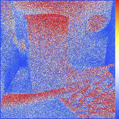
Sliced Optimal Transport Sampling • 1:7

       Iter.
         Disk
        Square
        Disk+mapping   1                  4                   16                  64                  256                   4096                  16384

Fig. 6. From random to SOT samples for uniform density. Starting from a random distribution of 1024 samples over a disk (top left) or a square (middle
left), iterating batches of 64-slice optimizations (left to right, up 16384 iterations) improves the uniformity of the samples, with no further visual improvement
after 300 iterations. If we map our disk distribution (top) onto the square (bottom) via our area-preserving deformation, we observe a very good approximation
of the square-based distribution which no longer requires the evaluation of a Radon transform over the square.

this modified 1D treatment with the vanilla one: alternating multi-                 in the full high dimensional space, and K/2 directions uniformly
class 1D steps with regular ones until convergence or a maximum                     distributed within each of the k projective subspaces. Since a good
iteration count results in both high class distribution quality and                 projective uniformity on the d-ball does not equate a good projective
global uniformity as seen in Figure 5.                                              uniformity after mapping onto the d-cube, we add a modification of
                                                                                    our computation of displacements: for each projective direction, we
3.6   Projective SOT sampling for rendering                                         project the current samples onto its associated 2D subspace, map
                                                                                    them to the corresponding 2-ball, and perform the SOT estimate of a
   Another variant of our SOT sampling targets rendering specifi-
                                                                                    displacement vector per sample there; we then map all the displace-
cally. As we discussed early on, Monte Carlo integration is particu-
                                                                                    ments back onto the d-cube using the inverse map. When all these
larly relevant to light transport simulation: rendering requires the
                                                                                    displacements for all subspaces and the entire space are computed,
estimation of an integral over all light paths within a scene con-
                                                                                    we average them to deduce a total displacement per sample as in
necting the camera sensor to light sources [Veach 1997]. However,
                                                                                    the vanilla SOT optimization procedure. This averaging can even
the integrand in this case has a particular structure that our SOT
                                                                                    be made dependent on the subspaces: one can for instance weight
sampling approach can further exploit. To simulate light bouncing
                                                                                    the displacements proportionally to the dimensionality (or respec-
k times over surface elements of a 3D scene, radiance must be in-
                                                                                    tively, the inverse thereof) of their associated subspace to induce a
tegrated over a 2k-dimensional space. Furthermore, the radiance
                                                                                    stronger preference for equidistribution in high (respectively, low)
reaching the camera can be integrated over its aperture to simulate
                                                                                    dimensional spaces. This modified optimization procedure, iterated
depth-of-field effects, over its sensor to avoid anti-aliasing, and over
                                                                                    until convergence or a maximum iteration count, allows for a bal-
time to handle motion blur. While this integration requires well
                                                                                    ance between full-space equidistributions and equidistributions in
distributed samples over the entire high-dimensional space, it can
                                                                                    the chosen subspaces and their combinations. Other strategies with
be beneficial to distribute samples uniformly within each of these k
                                                                                    a different balance between various properties could be derived
subspaces as well (i.e., for each possible path length): both Reinert
                                                                                    as well, but we found this simple variant (that we call “projective”
et al. [2016] and Perrier et al. [2018] have proposed techniques to
                                                                                    sliced optimal sampling) quite efficient as is. We will demonstrate
enforce a blue noise or Poisson disk property not only in a high
                                                                                    its efficacy in Sec. 4.4 for rendering purposes.
dimensional path space d, but also in each 2-dimensional pair or
combinations of dimensions.
   Our method easily supports a similar functionality by performing                 4    RESULTS
optimization steps using projection directions lying within these                      We now present a series of numerical tests to ascertain the proper-
subspaces. For a given choice of path-space dimension 2k (typically,                ties of our new SOT sampling method. While performing an exhaus-
we pick 6D or 8D), we initialize n samples in this high dimension                   tive analysis of Monte Carlo integration with SOT samples in high
through random sampling of a uniform density. Then, for each step                   dimensions is unsurmountably difficult, we study its behavior from
of our minimization, we pick a set of directions from the full space                a variety of perspectives, including visual inspection and spectral
as well as from the target projections in orthogonal two-dimensional                analysis in low dimensions, numerical accuracy and convergence for
subspaces: we randomly pick K directions uniformly distributed                      both low and high dimensions, as well as computational efficiency.

                                                                                                ACM Trans. Graph., Vol. 39, No. 4, Article 1. Publication date: July 2020.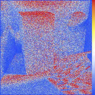
1:8 •   Paulin, et al.

4.1     Low-dimensional SOT sampling
   We first provide visual and numerical evaluations of our results
in low dimensions to better understand their basic properties.

      Disk                      Square                    Disk+mapping

Fig. 7. 2D Fourier spectrum. Whether a SOT sampling with 4K samples
is generated on a disk, directly on a square, or via mapping from a SOT
sampling of the disk to the square, its power spectrum and radial mean           Fig. 8. 4D radial spectra. (top) Radial power spectra comparison in dimen-
power spectrum clearly exhibit all the hallmarks of blue noise distributions —   sion 4 of 4K samples for various samplers; note that while dart throwing
with additional artifacts due to boundary alignment and/or mapping effects       exhibits a stronger peak than SOT, its behavior at low frequencies is also
on a square domain. Note that the (radial mean) power spectrum for the           significantly worse than all others (bottom) With a random initialization,
disk case was computed using only samples within the square inscribed in         the radial power spectra of SOT sampling goes from a white-noise shape to
the disk to allow for a proper discrete Fourier transform.                       a more blue-noise one during optimization.

  SOT iterations in 2D. Fig. 6 shows how a 2D pointset, initialized                 Spectral properties in 4D. As a first foray into higher dimensions,
through random sampling of a uniform distribution, evolves as                    we show in Fig. 8 how our SOT optimization in 4D improves the
SOT iterations of 64-slice displacements are performed, for both                 spectrum of a sample distribution (computed via a 4D fast Fourier
a disk (top) and a square (middle) domain. The disk domain uses                  transform of the unit 4-cube) as K-slice batches are performed, still
our uniform sampling method over balls as described in Sec. 3.3,                 using a random initialization of the samples for illustration purposes.
while the square domain uses a more general – thus more costly –                 The profile goes from flat at very early stages, to blue noise. Finally,
numerical evaluation of a (partial) Radon transform over the domain.             we demonstrate that other usual sampling techniques (dart throwing,
After around 256 iterations, the pointsets have visually converged.              Sobol, or jittered grids) do not exhibit a similar profile in 4D (top).
   Mapping effects. Still in Fig. 6 (bottom), we also display a SOT              4.2   Integration accuracy for SOT sampling
sampling in a square domain computed from the disk sampling
result via our disk-to-square map as explained in Sec. 3.4. While                   The main goal of our work is to provide an efficient way to create
the resulting pointset based on the map is not as well distributed               high-dimensional pointsets for which constant-weight quadrature
as the properly evaluated sliced optimal transport sampling, the                 evaluations offer improved accuracy compared to existing methods.
former does not result in obvious directional alignments, and scales             We thus performed a number of numerical evaluations, using simple
far better to high dimensions in terms of computational complexity.              Gaussian functions and other analytical integrands, to evaluate how
                                                                                 our approach fares compared to a regular Monte Carlo method or
   Spectral properties in 2D. As a means to evaluate SOT sampling                to quasi-Monte Carlo methods.
compared to previous blue noise sampling methods, we also provide
in Fig. 7 the power spectrum, computed via averaging over angles,                   Smooth functions in low & high dimensions. In Fig. 10 (left), we test
of a sliced optimal transport pointset in a 2D square generated
                                                                                 the accuracy of Monte Carlo integration
                                                                                                                           for a multivariate Gaussian
via mapping. The resulting spectrum is, as expected, close to the                distribution of the form д(x) = exp − 12 (x − µ)T Σ−1 (x − µ) , where
characteristic blue noise profile. In particular, we observe the telltale        we constrain the mean vector to satisfy 0 < µ i < 1 and the covariance
behavior near the DC component where the spectrum remains flat                   matrix so that each eigenvalue is at least 0.06 and at most 0.15.
for a large frequency band, and a white noise at high frequencies.               For each curve, we average the integration errors over the same
Compared to other blue noise methods such as [De Goes et al. 2012],              1024 randomly-selected Gaussians to offer a less noisy visualiza-
we also exhibit a peak at the characteristic frequency, but observe a            tion, but depict the minimum and maximum errors from these 1024
minor anisotropy of the spectrum due to the distortion induced by                integrations to offer an evaluation of the error variance. A typical
the disk-to-square mapping.                                                      multivariate Gaussian distribution used in our integration tests is

ACM Trans. Graph., Vol. 39, No. 4, Article 1. Publication date: July 2020.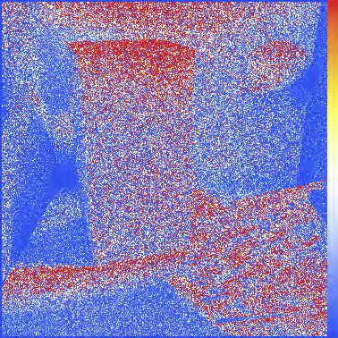
Sliced Optimal Transport Sampling • 1:9
Dimensions {1, 2} Dimensions {3, 4} Dimensions {5, 6}
Power spectrum Radial mean Power spectrum Radial mean Power spectrum Radial mean
Sobol+Owen
1.4 1.4 1.4
1.2 1.2 1.2
1 1 1
0.8 0.8 0.8
0.6 0.6 0.6
0.4 0.4 0.4
0.2 0.2 0.2
0 0 0
0 0.5 1 1.5 2 0 0.5 1 1.5 2 0 0.5 1 1.5 2
[Reinert et al. 2016]
1.4 1.4 1.4
1.2 1.2 1.2
1 1 1
0.8 0.8 0.8
0.6 0.6 0.6
0.4 0.4 0.4
0.2 0.2 0.2
0 0 0
0 0.5 1 1.5 2 0 0.5 1 1.5 2 0 0.5 1 1.5 2
1.4 1.4 1.4
1.2 1.2 1.2
SOT
1 1 1
0.8 0.8 0.8
0.6 0.6 0.6
0.4 0.4 0.4
0.2 0.2 0.2
0 0 0
0 0.5 1 1.5 2 0 0.5 1 1.5 2 0 0.5 1 1.5 2
Proj. SOT
1.4 1.4 1.4
1.2 1.2 1.2
1 1 1
0.8 0.8 0.8
0.6 0.6 0.6
0.4 0.4 0.4
0.2 0.2 0.2
0 0 0
0 0.5 1 1.5 2 0 0.5 1 1.5 2 0 0.5 1 1.5 2
Fig. 9. Fourier spectra on projections. In dimension 6 with 8K samples, we compare our projective SOT sampling (bottom) to other techniques such as
Projective Blue Noise [Reinert et al. 2016] to enforce good projective distributions in dimensions {1, 2}, {3, 4} and {5, 6}. The power spectra and radial
mean for these 2D projections demonstrate the quality of our projective SOT variant, and highlights that Owen-scramble Sobol sampling exhibits significant
artifacts in these subspaces, while our vanilla SOT shows an expected white noise distribution.
shown in the inset. Monte Carlo integration Discontinuous functions in low & high dimensions. In order to ex-
using our SOT sampling performs far better plore the numerical behavior of our sampling strategy more broadly,
than integration using Sobol or Sobol with we also tested the accuracy of MC integration for discontinuous
Owen scrambling for 100 samples and above functions. As a representative example, we chose a simple Heaviside
in this 2D test. We even consistently outper- (fn (p) = 1 if p · n > 0, 0 otherwise) function to show our robustness
form the recent PMJ02 method of Christensen to discontinuities. The same error plot as above (with this time, 1024
et al. [2018b]. This superior behavior holds different Heaviside with each a randomly-selected normal n) do not
true in 4D and 6D with a reduced margin of improvement. The same exhibit large differences between our SOT sampling and traditional
test in dimension 20 shows that we still outperform Sobol with Owen QMC methods: as Fig. 10(right) indicates, this class of functions
scrambling. All Sobol initialization vectors were taken from [Joe and is not really well handled by either, consistent with the expected
Kuo 2008], in the same order. For completeness, we also included in absence of theoretical error bounds in this case. Yet, SOT sampling
all our graphs an example of optimized low-discrepancy pointsets: performs as well as, or at times slightly better than, Sobol with
we used rank-1 lattices [Keller 2004] generated via the implementa- Owen scrambling — even in dimension 20.
tion of [L’Ecuyer and Munger 2016]. As a side note, rank-1 samples
may happen to have toroidal symmetry over the unit domain due 4.3 Computational complexity of SOT sampling
to their lattice nature, and this special configuration is known to Our algorithm for SOT sampling generation requires the prior
lead to exponential convergence for the integration of smooth and selection of two parameters: the number of slices K and the total
periodic functions; our choice of functions purposely prevents this number of batches. In order to evaluate a good strategy to automat-
case, which would have otherwise been not representative of the ically set these parameters, we plotted the SOT energy of a pointset
typical use of numerical integration in higher dimensions. as a function of batch and slice numbers. For all dimensions up to 20,
it indicates that there is virtually no numerical advantage in using
ACM Trans. Graph., Vol. 39, No. 4, Article 1. Publication date: July 2020.
1:10   •   Paulin, et al.

                                        Gaussian integrands                                             Heaviside integrands
              2D
              4D
              6D
              20D

Fig. 10. Monte Carlo integration on canonical functions. We consider various integration tests in dimensions 2, 4, 6, and 20 to evaluate MC integration
error as a function of the number of samples n. The Gaussian integrands (left) column depicts the error averaged over 1024 integrations of random multivariate
Gaussian distributions in the [0, 1)d domain; each solid curve indicates this error for a different sampler, and the associated shaded region indicates the
max and min error over the 1024 integral evaluations. The Heaviside integrands (right) column depicts the error averaged over 1024 integrations of random
Heaviside functions going through the center of the [0, 1)d domain; the same visualization of min, mean, and max errors is used. Note that Orthogonal Arrays
refers to the CMJND sampler of [Jarosz et al. 2019], while PMJ02 refers to the method of [Christensen et al. 2018b].

ACM Trans. Graph., Vol. 39, No. 4, Article 1. Publication date: July 2020.
Sliced Optimal Transport Sampling • 1:11
a
b a
c b
c a
b
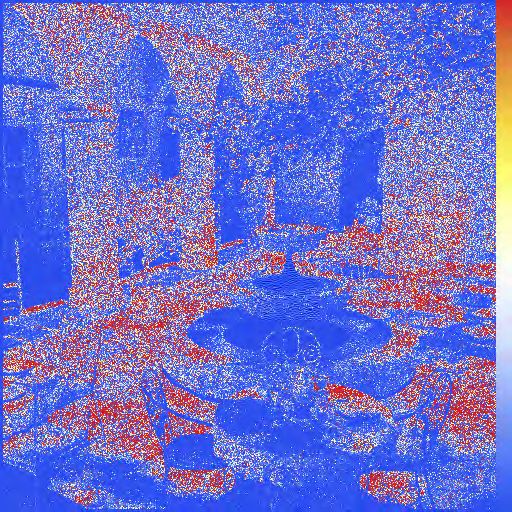
(I) Cornell scene, one bounce (II) Cornell scene, two bounces (III) Cloud rendering, two bounces
Fig. 11. Reference scenes used in our rendering experiments. For the Cornell test, we use either (I) indirect lighting with only one bounce (thus requiring
6D samples), or (II) two bounces (needing 8D samples); highlighted windows (marked as a, b, and c in each case) are 7×7-pixel regions used for convergence
plots in Figs. 12 and 15 respectively. For our cloud scene with a participating medium (III), we render two light bounces in PBRT, using 8D samples (2D for rays
initialization in screen-space, and 3D per bounce to sample depth and direction of each light–medium interaction); highlighted windows (marked as a, and b)
are 16×16-pixels areas used for convergence plots in Fig. 17.
(a) (b) (c)
Fig. 12. Convergence plots for 6D. For the three pixel windows depicted in Fig. 11(a), we plot the graphs of absolute errors as a function of sample count.
more than 64 slices (see inset for 4.4 Rendering with SOT sampling
the case of dimension 6; all other Integrations performed in the context of rendering are very spe-
dimensions are similar up to scale). cific, so we proposed a variant of our sliced optimal transport ap-
We therefore use K = 64 in all our proach by designing samples equidistributed in high dimensions
results. The number of batches as well as in select subspaces. A first way to evaluate the quality
needed to reach a near optimal of the pointsets we generate for rendering purposes is to examine
SOT energy is also quite indepen- 2D projections of the samples in order to evaluate their equidis-
dent of the dimension; we thus tribution in the most relevant subspaces. Fig. 9 shows the spectra
used 4096 batches for all dimensions up to 20. Higher dimensions and radial spectra of each 2D projection for a 6D projective SOT
may require, instead, a stopping criterion based on the magnitude of sampling, generated with a weighting of respectively 2 and 1 for the
energy decrease for improved accuracy. With these two parameters full dimensional 6D space and each of the 2D projective subspaces.
fixed, we provide an evaluation of the typical performance of our Compared to [Reinert et al. 2016], we observe a much improved
algorithm in Fig. 18: we depict our running times as a function of the projective behavior, with a clear absence of frequencies near DC.
number n of samples and as a function of the spatial dimension d. Note that a similar illustration in 4D is given in our supplemental
We observe clearly an O(d) complexity, with odd dimensions being material (as well as additional visualizations of 2D projections of
slightly faster to handle than even dimensions because of hypergeo- 6D samples), and the improvements are equally clear.
metric function evaluations. We also see a quasilinear dependence to
the number of samples as expected from our repeated 1D sorts. The We also tested the efficacy of this projective variant on three
time required to compute the sphere-to-cube mapping is negligible rendering scenes: the purposely simple Cornell test (Figs. 11 (I)
compared to the optimization steps, as it only involves a maximum and (II) show the two viewpoints we will use, in which small 7×7-
of 0.01% of the total computational time. Finally, a typical running pixel windows are marked as test regions of increasing complexity
time for 16K samples in 8D using 4096 optimization batches of 64 for error convergence plots), the more involved San Miguel scene
slices each is below 10 seconds on an AMD Ryzen Threadripper (Fig. 1), and a volumetric rendering of a cloud (Fig. 11(III)). For
2990WX with 32 cores at 3 GHz. the Cornell scene, Fig. 13 shows the spatial distribution (per-pixel
ACM Trans. Graph., Vol. 39, No. 4, Article 1. Publication date: July 2020.1:12 • Paulin, et al.
4spp 8spp 16spp 32spp 64spp 128spp 256spp 512spp 1024spp 2048spp 4096spp
Dart throw.
Sobol
Rank-1
oj. SOT
Proj.
Sobol
Rank-1
SOT
oj. SOT
Proj.
oj. SOT CR
Proj. oj. SOT CR
Dart throw. White noise Proj.
Fig. 13. Rendering results in dimension 6. We render the Cornell scene with one bounce of indirect lighthing using various samplers and for several
sample counts. To highlight the efficiency of Monte Carlo integrations, we display the error maps (per-pixel absolute difference with reference image in Fig. 11)
using pseudocolors (from blue to red, with a linear map from 0 to 0.002/spp). While SOT sampling does not help much for rendering, its projective variant is
better and/or more consistent than other typical approaches, particularly so for low counts of samples per pixel.
ACM Trans. Graph., Vol. 39, No. 4, Article 1. Publication date: July 2020.Sliced Optimal Transport Sampling • 1:13
4spp 8spp 16spp 32spp 64spp 128spp 256spp 512spp 1024spp 2048spp 4096spp
Dart throw.
Sobol
Rank-1
Dart throw. White noise Proj. SOT CR
Sobol
Rank-1
Proj. SOT CR
Fig. 14. Rendering results in dimension 8. We render the Cornell scene for two bounces of indirect lighthing using various samplers and for several
sample counts. The same visualization as in Fig.13 is used, but now compared to the reference image in Fig. 11(b) and with a linear map from 0 to 0.001/spp.
(a) (b) (c)
Fig. 15. Convergence plots for 8D. For the three pixel windows depicted in Fig. 11(right), we plot the graphs of absolute errors as a function of sample count.
ACM Trans. Graph., Vol. 39, No. 4, Article 1. Publication date: July 2020.1:14 • Paulin, et al.
4spp 8spp 16spp 32spp 64spp 128spp 256spp 512spp 1024spp 2048spp 4096spp
Dart throw.
Sobol
Rank-1
Dart throw. White noise Proj. SOT CR
Sobol
Rank-1
Proj. SOT CR
Fig. 16. Volumetric rendering results in 8 dimensions. We render a cloud-like participating medium, simulating two medium interactions (bounces) using
various samplers and for several sample counts. Samples are 8-dimensional: 2D screen space and two bounces using 2+1D for each bounce direction and depth.
As in Fig.14, error maps (per-pixel absolute difference with reference image in Fig. 11) use pseudocolors from blue to red, with a linear map from 0 to 0.002/spp.
Full image (a) (b)
Fig. 17. Convergence plots for 8D volumetric. From left to right: convergence of the full image, and of the 16 × 16-pixels areas highlighted in Fig. 11. The
main curves represent the mean absolute error of 8 independent realizations (when applicable) while the encasing auras represent the bounds of the mean
absolute error over the 8 independent realizations.
ACM Trans. Graph., Vol. 39, No. 4, Article 1. Publication date: July 2020.Sliced Optimal Transport Sampling • 1:15
These tests demonstrate that our projective SOT approach rivals
optimized pointsets such as rank-1 in quality and can lead to no-
ticeable gains compared to low-discrepancy sequences for less that
1000 samples, with the difference basically vanishing for larger sizes.
While complex regions do not benefit much from our SOT sampling,
less complex regions are often estimated with a lower error. Note
that our supplementary material provides further visual results for
completeness. We also observe uneven errors for Sobol sampling in
all rendering cases: these errors are highly structured with blocky
appearances that can be linked to uneven stratification in several
dimension pairs for some sample numbers, see Fig. 12 in our Supple-
Fig. 18. Performance. To assess the efficiency of our algorithm, we plot mental material. Rank-1 sampling is also uneven in quality, although
its computational cost as a function of the number of samples (left, for
less so: Fig. 13 shows that 4096spp behaves noticeably worse than
dimensions 2 and 8), and as a function of the dimension (for 16K samples).
2048spp, while Fig. 14 does not show such an artifact — and in
We used 4096 batches of 64 slices for both graphs.
fact, outperforms projective SOT at high spp for this particular case.
Our supplementary material provides visual evidence of spurious
absolute difference with the reference image) of various samplers alignments in several dimension pairs as well in Figs. 19, 22 and 23.
when indirect lighting with only one bounce (i,e., using samples
in 6D generated as described above) is simulated, whereas Fig. 14 5 CONCLUSIONS
simulates two bounces (i.e., using samples in 8D, still with the same Our proposed sliced optimal transport strategy for point sam-
weighting strategy, but there is now one additional 2D subspace). pling generation efficiently constructs, in low or high dimension,
For our volumetric rendering shown in Fig. 16, we also use 8D pointsets with good uniformity properties with respect to either a
samples to handle two bounces: our projective SOT pointsets are constant or variable density probability function. When using these
optimized to sample both the whole 8D space as well as the 3D samples for Monte Carlo integration, we observe reduced integra-
spaces of bounces, the 2D spaces of directions, and the 1D spaces of tion error compared to quasi-Monte Carlo approaches. Surprisingly,
depths; the subspaces (1, 2, 3, 4, 5, 6, 7, 8), (1, 2), (3, 4, 5), (6, 7, 8), (3), our approach is an order of magnitude better on smooth integrands
(4, 5), (6), and (7, 8) are weighted respectively 4, 1, 2, 2, 1, 1, 1, and than most low-discrepancy sequence strategies, known as the fastest
1 during our projective optimization procedure. The participating variance reduction approaches for QMC.
medium we use has an isotropic phase function and its density
field derives from a closed-form representation [Bálint and Mantiuk Limitations. As we designed our sampling approach to reduce
2019] encased inside a spherical domain and modified to allow integration error, the support of the density distribution as well as
gaps of zero density. Such a representation allows for a closed-form the boundary of the domain of integration Ω affects our sample dis-
expression of the transmittance over the interval of a ray–medium tributions: in a square for instance (Fig. 6, second row), we see that
intersection, which in turn lets us apply closed-form tracking [Novák a layer of points has formed along the border. While this benefits
et al. 2018] to sample the depth of the interaction over the same finite the integration accuracy by improving the sampling of the “discon-
interval. We provide results for sample counts varying from 4 to tinuity” that the border creates, it may be detrimental if our samples
4096. We tested our projective SOT sampling in two different ways. are used for other purposes such as stippling. At this moment, we
We first tried a straightforward strategy where each pixel randomly do not have a clear understanding of how these boundary samples
selects a realization of projective SOT sampling; we denote this affect practical applications and spectral properties.
approach as “Proj. SOT”. We also tested adding a micro-Cranley- Future work. This work raises a number of interesting questions,
Patterson rotation per pixel, i.e., toroidal translations using random both on the practical front and from a theoretical standpoint. Con-
vectors of length (2 · spp)−1 (larger translations may alter the quality vergence of our SOT optimization may become slow in very high
of non-toroidal samplers like ours [Singh et al. 2019]), to enrich dimensions (see Supplemental Material for statistics); if scalabil-
the projective SOT realizations; this second aproach is denoted ity is important, it might be interesting to explore how a faster
“Proj. SOT CR” in our results. The results show reduced errors for convergence of our minimization could be obtained through more
our sampling, at times significantly, compared to the traditional advanced numerical techniques than simple iterated averages of
use of Sobol with Owen scrambling. We also rival, and sometimes sliced transport optimizations. The design of other ball-to-cube
outperforms, rank-1 sampling — although rarely on large sample maps minimizing different forms of distortion would also be of
counts. Note that our tests used one global Sobol pointset for the value. Additionally, while our projective sampling approach was
entire image (leveraging its stratification property), while the other already proven valuable for rendering applications, we believe that
samplers were used locally (per pixel), with toroidal translations for a more systematic evaluation of weighting strategies in our projec-
rank-1 and Proj. SOT CR. tive variant (maybe guided by the weights used in [L’Ecuyer and
Finally, we also provide convergence plots on three different Munger 2016] or [Reinert et al. 2016]) could result in appreciable
7 × 7 test windows, from both the one- and two-bounce cases of gains. Moreover, there may be a number of other contexts for which
the Cornell scene in Figs. 12 and 15 respectively, and on two dif- an extension of our projective variant could be valuable. In par-
ferent 16 × 16 test windows from the volumetric scene in Fig. 17. ticular, more complex constructions of generalized projective SOT
ACM Trans. Graph., Vol. 39, No. 4, Article 1. Publication date: July 2020.You can also read