Snub nosed monkeys (Rhinopithecus): potential distribution and its implication for conservation - Pure
←
→
Page content transcription
If your browser does not render page correctly, please read the page content below
Biodivers Conserv (2018) 27:1517–1538
https://doi.org/10.1007/s10531-018-1507-0
ORIGINAL PAPER
Snub‑nosed monkeys (Rhinopithecus): potential
distribution and its implication for conservation
Jonas Nüchel1,2 · Peder Klith Bøcher1 · Wen Xiao3 · A‑Xing Zhu4,5,6 ·
Jens‑Christian Svenning1,7
Received: 2 October 2016 / Revised: 9 January 2018 / Accepted: 17 January 2018 /
Published online: 23 January 2018
© The Author(s) 2018. This article is an open access publication
Abstract Many threatened species have undergone range retraction, and are confined to
small fragmented populations. To increase their survival prospects, it is necessary to find
suitable habitat outside their current range, to increase and interconnect populations. Spe-
cies distribution models may be used to this purpose and can be an important part of the
conservation strategies. One pitfall is that such mapping will typically assume that the cur-
rent distribution represents the optimal habitat, which may not be the case for threatened
species. Here, we use maximum entropy modelling (Maxent) and rectilinear bioclimatic
envelope modelling with current and historical distribution data, together with the location
of protected areas, and environmental and anthropogenic variables, to answer three key
questions for the conservation of Rhinopithecus, a highly endangered genus of primates
consisting of five species of which three are endemic to China, one is endemic to China
Communicated by David Hawksworth.
Electronic supplementary material The online version of this article (https://doi.org/10.1007/s105
31-018-1507-0) contains supplementary material, which is available to authorized users.
* Jonas Nüchel
j.nuchel@bios.au.dk; j.nychel@live.com
1
Section for Ecoinformatics & Biodiversity, Department of Bioscience, Aarhus University, Ny
Munkegade 114, 8000 Aarhus, Denmark
2
Sino-Danish Center for Education and Research, Beijing 100101, China
3
Institute of Eastern‑Himalaya Biodiversity Research, Dali University, Dali 671003, Yunnan, China
4
School of Geography, Nanjing Normal University, Nanjing 210023, Jiangsu, China
5
State Key Laboratory of Resources and Environmental Information System, Institute
of Geographical Sciences and Natural Resources Research, Chinese Academy of Sciences,
Beijing 100101, China
6
Department of Geography, University of Wisconsin-Madison, 550 North Park Street, Madison,
WI 53706, USA
7
Center for Biodiversity Dynamics in a Changing World (BIOCHANGE), Aarhus University, Ny
Munkegade 114, 8000 Aarhus, Denmark
13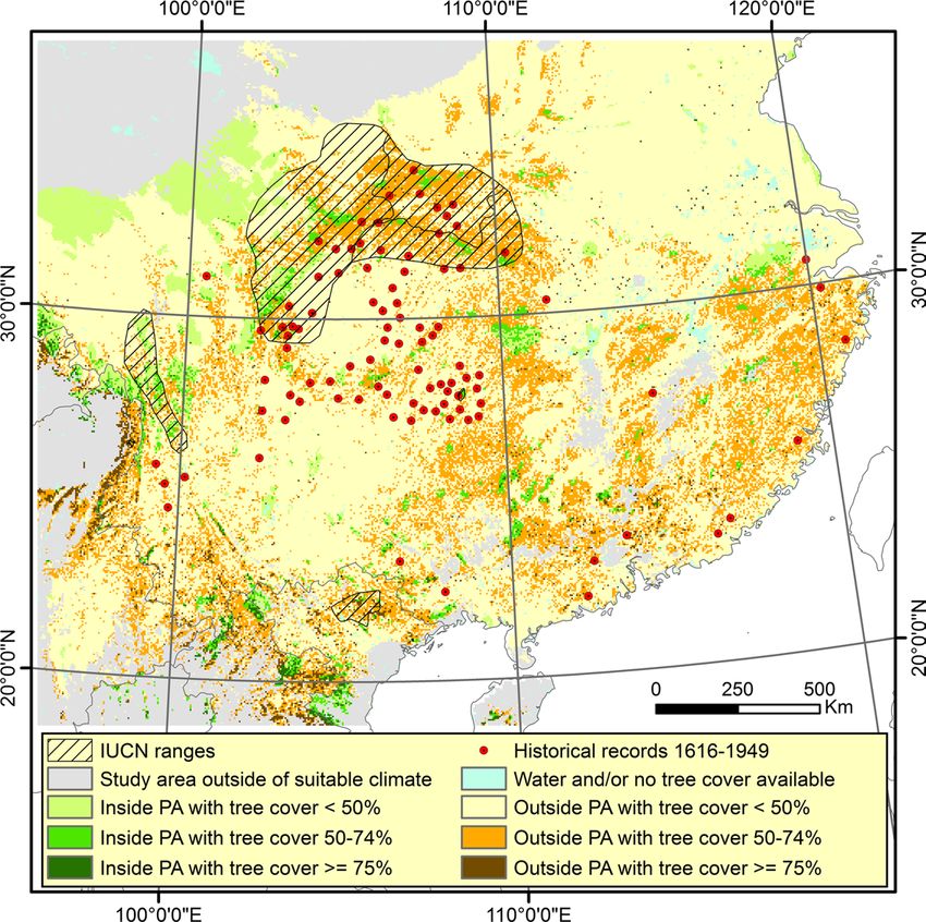
1518                                                     Biodivers Conserv (2018) 27:1517–1538

and Myanmar and one is endemic to Vietnam; Which environmental variables best predict
the distribution? To what extent is Rhinopithecus living in an anthropogenically truncated
niche space? What is the genus’ potential distribution in the region? Mean temperature of
coldest and warmest quarter together with annual precipitation and precipitation during the
driest quarter were the variables that best explained Rhinopithecus’ distribution. The his-
torical records were generally in warmer and wetter areas and in lower elevation than the
current distribution, strongly suggesting that Rhinopithecus today survives in an anthropo-
genic truncated niche space. There is 305,800–319,325 km2 of climatic suitable area within
protected areas in China, of which 96,525–100,275 km2 and 17,175–17,550 km2 have tree
cover above 50 and 75%, respectively. The models also show that the area predicted as
climatic suitable using Maxent was 72–89% larger when historical records were included.
Our results emphasise the importance of considering historical records when assessing res-
toration potential and show that there is high potential for restoring Rhinopithecus to parts
of its former range.

Keywords Rhinopithecus · Snub-nosed monkey · Species distribution modelling ·
Historical distribution · Maxent · Conservation

Introduction

Around 28% of mammal species are threatened or near threatened with extinction (IUCN
2014). The main threats are habitat loss and habitat degradation, mainly due to anthropo-
genic pressure, and many species have had their ranges reduced and are today living in
small fragmented populations (IUCN 2008; Schipper et al. 2008). These species are there-
fore more vulnerable to further anthropogenic impacts, with the small population size also
itself constituting a threat, causing vulnerability to inbreeding, demographic stochasticity,
diseases and catastrophes (Caughley 1994). One of the main conservation tools is protect-
ing the existing habitat which threatened species inhabit (Joppa and Pfaff 2011; Juffe-Big-
noli et al. 2014). However, for species surviving only as small and fragmented populations
this may not be sufficient to ensure their survival. Hence, reintroduction may be used to
help enhance the long-term survival prospects for these species, by translocation of species
to suitable habitat outside its current range, for example previously occupied areas. Addi-
tionally, such reintroductions or otherwise assisted range expansions will be necessary to
restore the ecological functions of such species (Seddon et al. 2014; Svenning et al. 2016).
    Species distribution modelling (SDM) can be used to find potential or suitable habitat
outside the species current range, (e.g. Morueta-Holme et al. 2010; Kuemmerle et al. 2011;
Chatterjee et al. 2012; Naundrup and Svenning 2015). Many SDMs use only the current
distribution of the species and assume that the habitat within represents the best habitat
(Braunisch et al. 2008). However, many threatened species have undergone range decline
and might be refugee species, i.e., confined to living in suboptimal habitat due to anthro-
pogenic pressures (Kerley et al. 2012). In such cases, SDM, if based on current data from
refugee habitats, might misguide conservation management by assuming that remnant pop-
ulations are found in the most favourable habitat (Cromsigt et al. 2012).
    East Asia in general has high biodiversity, e.g. China ranks third in the world in total
number of mammal species (IUCN 2008; Smith and Xie 2008), it has a higher diversity of
species than either North America or Europe and around one-eighth of all know species on
earth (Harkness 1998). Unfortunately, the region also has a high proportion of threatened

13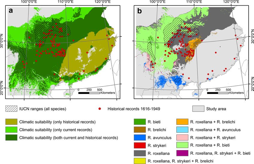
Biodivers Conserv (2018) 27:1517–1538                                                   1519

mammals (Schipper et al. 2008; Hoffmann et al. 2010). China has a long history of anthro-
pogenic impacts on its ecosystems and the impacts have grown drastically in the recent
century and especially the last decades, e.g. large areas of forest have been logged during
the last half century and the population in China has also more than doubled in the same
period (Harkness 1998; Liu and Diamond 2005). This also means that there is a high prob-
ability that many of the regions’ threatened species are refugee species, confined to sub-
optimal habitat. On the other hand, it should be noted that there are large reforestation and
afforestation programs going on in China, especially since end of 1990s (Yin et al. 2005;
Zhang and Song 2006; Peng et al. 2014; Nüchel and Svenning 2017).
   One of the organism groups with many threatened species are primates. Of the 508
known species of primates world-wide, 437 have been assessed by the International Union
for Conservation of Nature (IUCN) Red List and of these are more than 66% threatened or
near-threatened (IUCN 2016) and the primates in South and Southeast Asia has an even
more precarious conservation status, with around 79% threatened with extinction (Schip-
per et al. 2008). In this study, we focus on one group of East Asian threatened primates,
the snub-nosed monkeys (Rhinopithecus), comprising five species: Rhinopithecus bieti
(black (Yunnan) snub-nosed monkey), R. brelichi (grey (Guizhou) snub-nosed monkey), R.
roxellana (golden (Sichuan) snub-nosed monkey), R. strykeri (Myanmar (Burmese) snub-
nosed monkey) and R. avunculus (Tonkin snub-nosed monkey). All five species are listed
as endangered or critically endangered on the IUCN Red List, with all having decreasing
populations. Furthermore, R. brelichi, R. strykeri and R. avunculus are, with total popula-
tion sizes under 1000 individuals, on the brink of extinction (Bleisch et al. 2008; Bleisch
and Richardson 2008; Xuan Canh et al. 2008; Yongcheng and Richardson 2008; Liu et al.
2009; Xiang et al. 2009; Geissmann et al. 2012). However, while the distribution of Rhi-
nopithecus is small and fragmented today, fossil and historical records show that it histori-
cally has been widely distributed across South, East and Central China (Kirkpatrick 1995;
Li et al. 2002).
   The main threats for all five species are habitat loss and hunting (Bleisch et al. 2008;
Bleisch and Richardson 2008; Xuan Canh et al. 2008; Yongcheng and Richardson 2008;
Geissmann et al. 2012). In addition, future climate changes and increases in human popula-
tion and resource demand will likely increase pressure on all Rhinopithecus populations.
All Rhinopithecus species therefore face an uncertain future, and to increase their survival
chances it is necessary to increase their population size and distributions.
   In this study, we use species distribution modelling to identify which climatic factors
are associated with the current distribution of Rhinopithecus within East Asia. We then
assess the extent to which Rhinopithecus are refugee species, confined to an anthropogeni-
cally truncated niche space (Cromsigt et al. 2012), by incorporating historical records of
extirpated populations within the SDM. Finally, to identify areas that may be suitable for
reintroduction, we estimate the potential distribution of Rhinopithecus within the region,
considering climate, habitat availability and the locations of nature reserves.

Methods

Study region and distribution data

We used range maps from the International Union for Conservation of Nature (IUCN) for
all five Rhinopithecus species as current distribution data (IUCN 2014). We converted the

                                                                                  13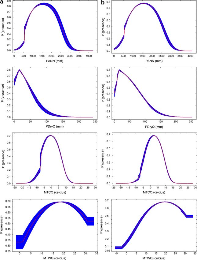
1520                                                             Biodivers Conserv (2018) 27:1517–1538

IUCN polygons to 5 × 5 km grid cells and then to one point per cell (centre of grid). The
range estimates were refined by excluding all points outside the species’ known elevation
ranges, which are between 200 and 1200 m for R. avunculus (Xuan Canh et al. 2008),
570 and 2300 m for R. brelichi (Bleisch et al. 2008), 1400 and 2800 m for R. roxellana
(Yongcheng and Richardson 2008), 1720 and 3190 m for R. strykeri (Geissmann et al.
2012), and 3000 and 4700 m for R. bieti (Bleisch and Richardson 2008). Furthermore, we
also excluded all areas with tree cover below 50%, all areas with human population density
above 100 and/or all areas with values above 20 on the human influence index (HII) (see
next section for explanation of HII). Afterwards, to reduce spatial bias, we used Occur-
rence Thinner version 1.04 (Verbruggen 2012; Verbruggen et al. 2013) to thin the points,
so we had 142 occurrence points within the IUCN ranges. In addition, historical records
for historically extirpated populations of Rhinopithecus in China were acquired from Li
et al. (2002). By digitalizing maps from Li et al. (2002), we derived 96 approximate loca-
tions for historical records from 1616 to 1949, including 70 locations outside the current
range of the genus (Fig. 1).
    The range data for all Rhinopithecus species were combined in most of our modelling
(i.e., modelling Rhinopithecus as a single taxon), mainly as the historical records could
not be identified into species level, but also to overcome niche truncation. All Rhino-
pithecus species, with the exception of R. avunculus, occur in subtropical to temperate for-
est (see Supporting Information Appendix S1 for map of ecoregions/vegetation zones) and

Fig. 1  Distribution of Rhinopithecus. IUCN range maps for all five species (R. strykeri, R. avunculus, R.
brelichi, R. roxellana & R. bieti) and historical records from 1616 to 1949

13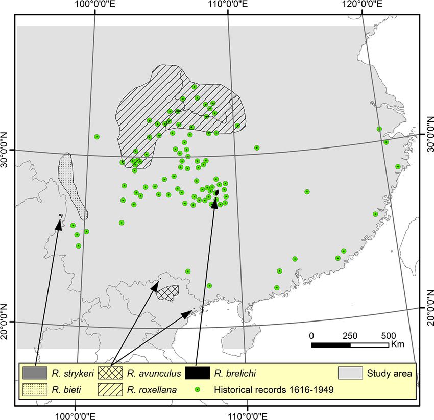
Biodivers Conserv (2018) 27:1517–1538                                                      1521

hence may be hypothesized to have similar ecological requirements. Rhinopithecus bieti,
R. strykeri, R. brelichi and R. roxellana mainly occur in mixed deciduous and evergreen
broadleaf forest, with R. bieti, R. strykeri, and R. roxellana also occuring in coniferous for-
est, and R. avunculus most deviant, being found in tropical evergreen forest (Bleisch et al.
2008; Bleisch and Richardson 2008; Xuan Canh et al. 2008; Yongcheng and Richardson
2008; Geissmann et al. 2012). Furthermore, Rhinopithecus has a high dietary plasticity and
occur in areas that have large variations in climate between summer and winter (Long et al.
1994; Yiming 2006; Guo et al. 2007; Xiang et al. 2007b, 2012; Grueter et al. 2009a; Wong
et al. 2013). Additionally, we also know that at least some of the species had a more wider
distributions as late as within the last 400 years (Li et al. 2002), also in areas that are more
climatic different than possibly unoccupied areas within the IUCN polygons. Moreover, as
stated in the introduction, some threatened species might be refugee species living in sub-
optimal habitats (Kerley et al. 2012; Cromsigt et al. 2012) and the current range might not
show their full climatic suitable range.
   The study area includes a part of East Asia, including areas in China, Myanmar and
Vietnam where Rhinopithecus are known to occur (Fig. 1). The study area was delimited
by drawing a rectangle around a 500-km buffer outside the species range maps and histori-
cal occurrence points.

Environmental and anthropogenic data

Multiple models were calibrated to identify which climate variables are most strongly
associated with the distribution of the genus. Initially, eight climatic variables from the
WorldClim database (Hijmans et al. 2005) were considered; (1) annual mean temperature
(AMT), (2) mean temperature of warmest quarter (MTWQ), (3) mean temperature of cold-
est quarter (MTCQ), (4) minimum temperature of coldest month (MinTCM), (5) annual
precipitation (PANN), (6) precipitation of wettest quarter (PWetQ), (7) precipitation of
driest quarter (PDryQ), (8) precipitation of coldest quarter (PColdQ). The four tempera-
ture variables, PANN, PDryQ and PWetQ were chosen due to their effect on vegetation
and thereby habitat. PColdQ was chosen because the monkeys, except R. avunculus and to
some degree R. brelichi, mainly live in high elevations and precipitation during the coldest
quarter will extensively fall as snow and possible limit the food availability.
   The historical records for extirpated populations of Rhinopithecus were mainly located
in Central East (CE) and Southeast (SE) China. We note that the temperature has varied
within the period of the historical records (1616–1949) and also subsequently up to the
present-day. Generally, the climate was colder in the period of the historical records, with
a maximum temperature difference between the coldest period (around 1660 and again
around 1840) and current temperature of 1.8 °C for CE China and 1.2 °C for SE China on a
decadal time series, and 0.7 °C for CE China and 0.6 °C for SE China on a centennial time
series (Ge et al. 2013). To investigate the possible effect of these temperature shifts and,
specifically, the colder period during the time of the historical records, we performed a
temperature sensitivity analysis by decreasing the current temperature with different mag-
nitudes, subtracting 0.7, 1.5 and 2.0 °C, respectively, from each of the current temperature
variables before calibrating the distribution models. The down-adjusted climate variables
were used to assess the sensitivity of the models to the different climate and compare the
results between models with different adjusted climate data.
   Furthermore, we used topographic data from Shuttle Radar Topography Mission
(SRTM) (Jarvis et al. 2008) for elevation (ELEV), and computed slope (Slope), standard
deviation (STD), and topographic roughness (slope of slope) (TR). Data for protected areas

                                                                                    13
1522 Biodivers Conserv (2018) 27:1517–1538
in China were derived from World Database on Protected Areas (IUCN and UNEP-WCMC
2014) and to capture tree cover we used the Moderate Resolution Imaging Spectroradiom-
eter (MODIS) Vegetation Continuous Fields from 2010 (DiMiceli et al. 2011).
We used two different measures of anthropogenic pressure to refine our current distri-
bution data; human population density for 2010 (CIESIN 2015) and the Human Influence
Index (HII) (WCS and CIESIN 2005). HII is an index going from 0 (no impact) to 64
(maximum impact) that combines data for population density with data for human land
use and accessibility (roads, railroads, navigable rivers and coastlines) and can be used to
describe anthropogenic impacts on the environment. The refining was done by excluding
all areas within the IUCN range maps with human population density above 100 and/or all
areas with values above 20 on the HII.
All data were projected to the Albers Equal Area Conic projection, and converted to
their mean values for 5 km × 5 km grid cells. ArcGIS 10.2 (ESRI, Redlands, CA) was used
for all GIS operations.
Maximum entropy modelling/distribution modelling
One of the modelling method used was Maximum entropy modelling (Maxent version
3.3.3k (http://www.cs.princeton.edu/~schapire/maxent/), which is a machine learning
method for mapping habitat suitability or estimate the potential distribution of a species
(Phillips et al. 2006; Phillips and Dudík 2008; Elith et al. 2011). Maximum entropy mod-
elling is among the best-performing methods for species distribution modelling and fre-
quently outperforms traditional statistical approaches and other species distribution model-
ling methods (Elith et al. 2006; Phillips et al. 2006).
Pairwise Pearson’s correlation coefficients (r) for all variables over the entire study area
were calculated (see Supporting Information Appendix S2 for r values) to quantify col-
linearity. Although Maxent is relatively robust against collinear variables, collinearity can
impair the estimation of the influence of individual variables on the model. Among the cli-
matic variables AMT was highly correlated with MinTCM (r = 0.98), MTWQ (r = 0.92),
and MTCQ (r = 0.96). AMT contributed less to the predictive power than MinTCM
and MTCQ, and was therefore not included in the modelling. Furthermore, MinTCM
and MTCQ were also highly correlated (r = 0.98) and were consequently only included
in mutually exclusive models. MTWQ was also correlated with MTCQ (r = 0.78) and
MinTCM (r = 0.85). MTWQ did not explain much of the variance, but provided a small
increase in predictive power and was therefore kept in four of the final models (Table 1).
PWetQ was strongly correlated with PANN (r = 0.94), with PANN contributing more to
predictive power than PWetQ; therefore PWetQ was removed. PDryQ and PColdQ were
also correlated (r = 0.98) and contributed almost equally to the predictive power. PDryQ
indicate the minimum amount of precipitation for a quarter and can be more of an indirect
stress factor for vegetation than PColdQ. Therefore, PColdQ was consequently removed.
Out of the four topographic variables, only ELEV contributed a little to the overall pre-
dictive power, with the rest having no influence at all. ELEV, STD, Slope and TR were
consequently left out of the final models. Both measure for anthropogenic pressure, human
population density for 2010 and HII were also left out of our final models, so our final
models only model climatic suitability (see Supporting Information Appendix S3, S4 and
result section for further).
The final variables in the models were PANN, PDryQ, MTWQ, and MinTCM or
MTCQ. This resulted in a total of four models, which were run with current distribution
13Table 1 The 2 × 4 models using only present distribution data from IUCN (CURR1–4) and also using historical records from 1616 to 1949 (HIST1–4), with variables used
and AUC, TSS, AICC and Akaike weight values
Biodivers Conserv (2018) 27:1517–1538
Presence data Model PA NN PDryQ Min TCM MT CQ MT WQ AUC TSS AICc Akaike weight Threshold
IUCN CURR1 X X X X 0.900 0.685 3148.094 1 0.320
CURR2 X X X X 0.896 0.662 3191.302 1.79 × 10⁻⁹ 0.364
CURR3 X X X 0.885 0.601 3207.430 5.62 × 10⁻¹³ 0.323
CURR4 X X X 0.878 0.624 3220.541 1.86 × 10⁻¹⁶ 0.370
HIST1 X X X X 0.835 0.576 4800.822 1 0.305
IUCN and histori- HIST2 X X X X 0.819 0.525 4841.374 2.91 × 10⁻⁹ 0.340
cal records HIST3 X X X 0.801 0.507 4855.961 8.86 × 10⁻¹³ 0.301
HIST4 X X X 0.793 0.515 4886.444 1.16 × 10⁻¹⁹ 0.330
1523
131524 Biodivers Conserv (2018) 27:1517–1538 data derived from the IUCN ranges and also with both current distribution data and histori- cal records from 1616 to 1949 (Table 1). Model tuning and evaluation We used area under the curve (AUC) of the receiver operating characteristics (ROC) curve to estimate the predictive power of our models. The maximum AUC value is 1, achieved by perfect discrimination between occupied and non-occupied cells, while a model with no better predictive ability than random choice will result in an AUC value of 0.5. In prac- tice, models with an AUC above 0.75 are considered potentially useful (Phillips and Dudík 2008). We note that for presence-only data, like in the present study, the highest achievable AUC is < 1 (Phillips et al. 2006). AUC values may not always be the optimal method to evaluate model performance, e.g. as AUC weighs omission and commission errors equally, and the geographical extent to which models are carried out in can highly influences the AUC values (Lobo et al. 2008). Therefore, the models were also evaluated using the true skill statistic (TSS), which in contrast to kappa is independent of prevalence (Allouche et al. 2006). TSS uses the same scale as kappa and has values between 0 and 1, where 0–0.4 = poor, 0.4–0.5 = fair, 0.5–0.7 = good. 0.7–0.85 = very good, 0.85–0.9 = excellent and 0.9–1 = perfect. In addition to TSS and AUC, we used the R package ENMeval version 0.1.1 (Mus- carella et al. 2014) to tune the features and regularization multiplier settings in Maxent, and ENMTools version 1.4.4 (Warren et al. 2008, 2010) to calculate the sample size corrected Akaike Information Criterion ( AICC) and Akaike weights value for our models. A ICC has been showed to outperform AUC-based methods for model selection in many cases (War- ren and Seifert 2010). The final models were run using default settings, except the regu- larization multiplier value, which was set to 2.5, maximum iterations was changed to 5,000 and all features were used. To derive suitability and predictive maps the final models were run 10 times with cross validate as replicated run type. Suitable habitat and potential distribution Our predictive presence-absence map was derived using the 10th percentile training pres- ence thresholds, which selects the value above which 90% of the training samples are cor- rectly classified. Selection of the best thresholds can be difficult and depends on the sam- ple size and the purpose of the study (Pearson et al. 2004; Liu et al. 2005; Freeman and Moisen 2008; Bean et al. 2012), but in general maximum training sensitivity and specific- ity, and equal training and specificity perform best (Jiménez-Valverde and Lobo 2007; Liu et al. 2013; Cao et al. 2013). The above thresholds are more conservative thresholds than the minimum training presence threshold, which correctly predicts every training sample (See Supporting Information Appendix S5 for a comparison of thresholds effect on our predictive presence-absence map). As an alternative, which is better protected against over- fitting, we also generated a rectilinear bioclimatic envelope model, defined as areas within minimum and maximum values of the five climatic variables, PANN, PDryQ, MinTCM, MTCQ and MTWQ, using only current distribution data derived from IUCN ranges and using both current distribution data and historical records, in ArcGIS. We did this for all species combined and also for each species separately. The latter was done to compare the species- and genus-level results, mainly for checking their consistency. Furthermore, the models with current and historical distribution data were modelled using both current 13
Biodivers Conserv (2018) 27:1517–1538 1525
climate data and current climate data adjusted with − 0.7, − 1.5, and − 2.0, respectively,
to provide estimates accounting for the cooler climate during the period that the historical
records represent.
To assess how much of the climatic suitable area includes tree cover above a certain
percentage and were within protected areas, the outputs from the rectilinear bioclimatic
envelope models were overlaid with tree cover, derived from Moderate Resolution Imag-
ing Spectroradiometer (MODIS) Vegetation Continuous Fields from 2010 (DiMiceli et al.
2011), and protected areas in China (IUCN and UNEP-WCMC 2014).
Results
The four models with current distribution data derived from IUCN ranges (CURR1-4,
Table 1) resulted in AUC values, between 0.878 and 0.900 and TSS values between 0.601
and 0.685, indicating good predictive power. The four models with both current distri-
bution data and historical records (HIST1-4, Table 1) resulted in AUC values, between
0.793 and 0.835 and TSS values between 0.507 and 0.576, again indicating good predictive
power. AICC and the derived Akaike weight scored the models with the variables PANN,
PDryQ, MTCQ and MTWQ, as the best models for both current data only (CURR1) as
well as for current and historical data together (HIST1). For all models, the ranks of the
models based on AICC and Akaike weights were consistent with the ranks/values of AUC
and to some degree also the values of TSS (Table 1).
Human population density for 2010 contributed to our the predictive power of our
models, whereas HII contributed only sligthly to the predictive power of our models (see
Suporting Information Appendix S3). The response curves from the Maxent model indi-
cate that there is a negative relationship between the current distribution of snub-nosed
monkeys and both of the anthropogenic variables, as the probability of presence in the
Maxent prediction decreased with increasing population density and HII (see Suporting
Information Appendix S3).
PANN, MTCQ or MinTCM, PDryQ and MTWQ were the variables that best explained
the distribution of Rhinopithecus (all five species modelled together). This was the case
when the distribution was modelled using current distribution data (derived from IUCN
ranges) as well as both current distribution data and historical records. However, the vari-
ables importance changes a little between model CURR1 and HIST1. For model CURR1,
using only current distribution data, the Maxent jackknife evaluation indicate that PDryQ,
followed by MTCQ and MTWQ were the strongest predictors by themselves. For model
HIST1, using historical data in addition to current distribution data, MTCQ, followed by
PANN and PDryQ were the strongest predictors. In both models, MTCQ was the variable
that decreases the gain the most when it was omitted, which indicate that it has the most
information that is not explained by the other variables (Fig. 2).
The estimated responses curves in Maxent had the same tendencies between model
CURR1 and HIST1, but with higher mean values for PANN, PDryQ, and MTCQ when
historical records were also included (Fig. 3). Consistent with the SDM results, the range
of the different environmental variables varied between the current distribution and the
historical records: All species, except R. avunculus, today generally occur in colder areas
and higher elevation than the historical records. This is also the case if the models are
calibrated using the down-adjusted temperature data to better match the historical cli-
mate reference (Fig. 4, and Supporting Information Appendix S6). Rhinopithecus roxel-
lana and R. bieti also generally occur in drier areas then the historical records (Fig. 4, and
131526 Biodivers Conserv (2018) 27:1517–1538 Fig. 2 Results of jackknife evaluation of the relative importance of the variables with respect to regularized training gain for (a) model CURR1 and (b) model HIST1. For acronyms see the environmental data section in methods Supporting Information Appendix S6). The medians for all climatic variables and elevation differed between the current distribution and the historical records (Mann-Whitney U tests, p < 0.0001). The areas predicted as climatic suitable using Maxent were 72–89% larger when his- torical records were also included (Fig. 5 and Table 2). The same tendencies were also obtained using rectilinear bioclimatic envelope modelling for all species together and the historical records (Fig. 6). However, the area predicted climatic suitable by the historical records in the models changed to some degree depending on which down-adjusted climate data that were used. The more down-adjusted climate data that were used, the less areas were considered climatic suitable. Primarily areas in South and South-central China were affected by the adjusted climate data (see Table 2 and Supporting Information Appendix S7 and S8 for comparison of the predicted area with the different adjusted climate data). The Maxent results were largely consistent with the rectilinear bioclimatic envelope models for the individual species (Fig. 6). The rectilinear bioclimatic envelope analy- ses at the genus level and including the historical records showed, depending on the his- torical climate adjustment used, that between 305,800 and 319,325 km2 of the climatic suitable area in China are within protected areas, of which 95,525–100,275 km2 has tree cover ≥ 50% and 17,1775–17550 km2 has ≥ 75% tree cover. In addition, there are between 738,425 and 824,425 km2 outside protected areas but with tree cover ≥ 50% and of these 57,350–62,100 km2 has tree cover ≥ 75% (Fig. 7 and Table 2, and Supporting Information Appendix S9). 13
Biodivers Conserv (2018) 27:1517–1538                                                              1527

Fig. 3  Estimated response curves (logistic output: probability of presence), which show how the logistic
prediction changes as each environmental variable is varied, keeping all other environmental variables at
their average sample value, for (a) model CURR1 and (b) model HIST1. For acronyms see the environmen-
tal data section in methods

Discussion

One or more species of Rhinopithecus were recently more widely distributed in China. All
species are today confined to fragmented areas with declining populations and are listed

                                                                                            13
1528 Biodivers Conserv (2018) 27:1517–1538 Fig. 4 Boxplot of elevation (ELEV), mean temperature of coldest quarter (MTCQ) and precipitation dur- ▸ ing driest quarter (PDryQ) for the historical records, the IUCN ranges (all five species together) and for the five species separately. See Supplementary Information Appendix S3 for boxplot of PANN, MinTCM and MTWQ. MTCQ for the historical records is divided into four categories; current climate data without adjustments, current climate data adjusted with − 0.7, − 1.5, and − 2.0 °C, respectively as endangered or critically endangered on the IUCN Red List (Bleisch et al. 2008; Bleisch and Richardson 2008; Xuan Canh et al. 2008; Yongcheng and Richardson 2008; Geiss- mann et al. 2012) and at least three of the species are, with total population sizes under 1000 individuals, close to extinction. In this study, we assessed three key questions for the conservation of Rhinopithecus: which climatic variables determine the current distribution of this genus, to what extent has the niche space of the genus been truncated due to anthro- pogenic activities, and what is the potential distribution of the genus, using species distri- bution modelling (SDM) with both current and historical distribution data. All the models scored AUC values between 0.793 and 0.900 and TSS values between 0.507 and 0.685, indicating good predictive power. PANN, MTCQ, MinTCM, PDryQ, and MTWQ were the variables that best explained the distribution of Rhinopithecus. There is a clear trend that the historical records generally are from areas that are warmer, wetter, and in lower eleva- tion then the current distribution records (except the ones from R. avunculus), indicating extensive niche truncation. This is the case regardless of whether the current climate data were down-adjusted by − 0.7, − 1.5, or − 2.0 °C. As such, models that included historical records projected climatically suitable habitat to occupy a larger geographic extent than models calibrated only with IUCN range data. This is the case using Maxent as well as rectilinear bioclimatic envelope modelling with different adjusted climate data. Based on the later, 74,525–79,650 km2 of the climatically suitable area has tree cover ≥ 75% and could therefore constitute suitable habitat for Rhinopithecus, hereof 17,175–17,550 km2 within protected areas. All Rhinopithecus species inhabit primary forest and grid cells with tree cover ≥ 75% might constitute important potential habitat. In addition, an additional 834,950–924,700 km2 climatically suitable area has tree cover between 50 and 75%, hereof 96,525–100,275 km2 within protected areas. This area may also be suitable ecologically, as Rhinopithecus species have been observed spending a considerable time on the ground feeding on fallen nuts, ground plants etc. (Long et al. 1994; Xiang et al. 2007b, 2012; Gru- eter et al. 2009a). The accuracy of the modelling depends on the accuracy of the distribution data. A prob- lem with accuracy of the distribution data may occur as the IUCN distribution polygons (IUCN 2014) we used as a basis for our current records undoubtedly include areas that are not currently inhabited by Rhinopithecus and may include areas that are outside the cur- rent realized climatic niche of the species. However, we reduce the risk of including areas beyond the current realized niche by excluding grid cells that are outside of the known elevation range of the genus, have low tree cover, or have high human population densities or human influence. Another problem regarding the possible inclusion of climate outside the current realized climatic niche of the species in the analyses is that we modelled all species together. However, the historical records could not be identified into species level and we can also see in the rectilinear bioclimatic envelope models for the individual spe- cies that it does not affect the overall result as they are in accordance with the rectilinear bioclimatic envelope model of the genus. Additionally, at least some of the Rhinopithecus species live in a fairly wide range of climates and have high dietary plasticity (Long et al. 1994; Yiming 2006; Guo et al. 2007; Grueter et al. 2009a; Xiang et al. 2007b, 2012; Wong 13
Biodivers Conserv (2018) 27:1517–1538                                                                                                                                                                                           1529

                                                     6000
                                                     5000
Elevation in meters
                                                     4000
                                                     3000
                                                     2000
                                                     1000
                                                     0

                                                            Historical              All IUCN              R. roxellana                    R. bieti              R. brelichi         R. strykeri           R. avunculus
                                                             records                 ranges

                                                                         Historical records
Mean temperature of coldest quarter (celcius)
                                                     15
                                                     10
                                                     5
                                                     0
                                                     -5
                                                     -10
                                                     -15

                                                              Ad               Ad                 Ad               Ad                IU              R.                R.            R.              R.               R.
                                                                jus              jus                jus              jus               CN                 rox               bie           bre             str              av
                                                                   ted               ted               ted              ted                  ran             ell               ti            lich            yk              un
                                                                         0.0               -0.               -1.              -2.               ge               an                              i              eri             cu
                                                                                              7                 5                0                   s             a                                                              lus
Precipitation during driest quarter in millimeters
                                                     200
                                                     150
                                                     100
                                                     50
                                                     0

                                                            Historical              All IUCN              R. roxellana                    R. bieti              R. brelichi         R. strykeri           R. avunculus
                                                             records                 ranges

                                                                                                                                                                                                                  13
1530 Biodivers Conserv (2018) 27:1517–1538
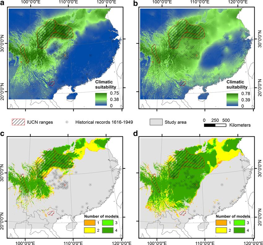
Fig. 5 Mean climatic suitability and predicted climatic distribution using ensemble intersection and the
10th percentile training presence threshold for the 2 × 4 models (Table 1) at a 5 km × 5 km resolution. a
Mean climatic suitability using only current range data and b using both current and historical data from
1616 to 1949. c Ensemble intersection for model CURR1–4 using only current range data and d for model
HIST1–4 using both current and historical data from 1616 to 1949. Colours indicate number of models
(ranging from 1 to 4) predicting values for climatic suitability above the 10th percentile training presence
threshold. No colour within the study area indicates that none of the models predicted values for climatic
suitability above the 10th percentile training presence threshold
et al. 2013). Moreover, both the Maxent and the rectilinear bioclimatic envelope model is
in accordance with the ecoregions, which distributions have been similar from the earli-
est historical records used (1616) to present (Ni et al. 2014) (see Supporting Information
Appendix S1).
Another aspect worth discussing is that China experienced a cold period between 1321
and 1920 (Ge et al. 2013), which to some extent coincides with the disappearance of
Rhinopithecus in southeast China. However, it does not make ecological sense that Rhi-
nopithecus should retreat to higher elevations and hence even colder conditions during a
period of increased cold. If temperature changes had affected its range dynamics in this
period, Rhinopithecus would logically have been expected to retreat to warmer areas, or
first retreat to the colder areas after 1920 when the current warm period began, i.e., both
scenarios in contrast to the observed pattern. Furthermore, Rhinopithecus also lived in
southeast China during the last warm period before 1321.
13Table 2 Area predicted (km2) by the Maxent models and the bioclimatic envelope models
Maxent models Bioclimatic envelope with current and historical records
Biodivers Conserv (2018) 27:1517–1538
Models CURR1–4 HIST1–4 Climate adjustedc Total area Within PA Within PA ≥ 50% Within PA ≥ 75% Outside PA ≥ 50% Outside PA ≥ 75%
Min. one modela 1,112,500 1,914,200 0.0 3,716,625 319,325 100,275 17,550 824,425 62,100
− 0.7 3,648,500 318,950 100,200 17,550 816,975 61,200
All four modelsb 705,275 1,336,300 − 1.5 3,420,100 313,100 98,600 17,300 774,675 58,575
− 2.0 3,284,275 305,800 96,525 17,175 738,425 57,350
a
Predicted by minimum one of the four models
b
Overlap of predicted area of all four models, CURR1–4 and HIST1–4 respectively
c
Climatic data used to model; 0.0 = current climate data without any adjustment, − 0.7, − 1.5, and − 2.0 = current climate data adjusted with − 0.7, − 1.5, and − 2.0 °C,
respectively
1531
131532 Biodivers Conserv (2018) 27:1517–1538
Fig. 6 Climatic suitable area, defined as area within minimum and maximum values of the five climatic
variables, PANN, PDryQ, MinTCM, MTCQ and MTWQ, at a 5 km × 5 km resolution. a Model for all
five species together, using only current data from IUCN ranges (light and dark green) and area included
if historical records is also used (brown green). Temperature data for historical records are adjusted with
− 0.7 °C (see Supporting Information Appendix S7 for other climate adjustments). b Climatic suitable
area, defined as area within minimum and maximum values of the five climatic variables, PANN, PDryQ,
MinTCM, MTCQ and MTWQ, at a 5 km × 5 km resolution for each species separately and the overlap
between them
Our analyses strongly suggest that the Rhinopithecus species now survive as refugee
species sensu Cromsigt et al. (2012). Comparing the SDM results with and without the his-
torical records show that there clearly has been truncation of the occupied environmental
space with respect to temperature and precipitation. The historical records are generally
from warmer and wetter areas, and in lower elevation than the current distribution. This
is also the reason why most of South, Southeast and Central China, which is warmer and
wetter than the areas where the species is found today, only is predicted as climatic suit-
able if the historical records are included in the analyses. Hence, the reason why a large
area in Southeast China is not predicted as suitable for Rhinopithecus, when only current
distribution data is used, is mainly due to too high levels of precipitation, likely reflect-
ing that high-rainfall areas have historically been more suitable for agriculture and human
settlement, with the disappearance of Rhinopithecus from these areas synchronous with
a rapid increase in human population and cultivated areas here during the last 400 years
(Durand 1960; Li et al. 2002). In contrast, we are not aware of any plausible mechanisms
whereby high rainfall would exclude Rhinopithecus directly or via non-anthropogenic indi-
rect effects. Today, Rhinopithecus are largely restricted to higher elevations than much
of their historical distribution. Li et al. (2002) provide evidence that Rhinopithecus was
first extirpated from lower elevation during the last 400 years. Higher elevation areas are
more remote and difficult for humans to access and utilize and other studies have found
less deforestation, more reforestation and afforestation, less range contraction, and less
13Biodivers Conserv (2018) 27:1517–1538 1533
Fig. 7 Climatic suitable area as defined in Fig. 6 outside protected areas (PA) (sand colors) and within pro-
tected areas (PA) (green colors). The darker sand or green color the higher tree cover percentage
extinction in topographically steep areas (Laliberte and Ripple 2004; Fisher 2011; San-
del and Svenning 2013; Faurby and Svenning 2015; Nüchel and Svenning 2017). Further-
more, many other species in the region, e.g., giant panda (Ailuropoda melanoleuca) and
red panda (Ailurus fulgens), have also been impacted by strong anthropogenic pressure
during the recent centuries with population declines and range retractions as consequences
(Ceballos and Ehrlich 2002; Zhu et al. 2010; Hu et al. 2011). As such, it is likely that Rhi-
nopithecus have been locally extirpated by anthropogenic factors, and are now restricted to
areas with higher elevation and which are less accessible, even though these may be subop-
timal habitats. Hence, Rhinopithecus is likely a refugee taxon, living in an anthropogenic
truncated niche space.
Even though our results show that there are large areas that are climatic suitable for the
genus, have tree cover between 50 and 75% or above 75%, and some even protected, it does
not mean that the species can actually live in these areas. For example, our modelling does
not show whether or not the vegetation meets the different Rhinopithecus species’ specific
requirements in terms of food and habitat structure. Today, R. avunculus is found in tropi-
cal evergreen (Xuan Canh et al. 2008). Rhinopithecus brelichi is found in mixed deciduous
and evergreen broadleaf (Bleisch et al. 2008; Xiang et al. 2009). Rhinopithecus roxellana
and R. strykeri is found in mixed deciduous and evergreen broadleaf and mixed conifer-
broadleaf forest (Guo et al. 2007; Yongcheng and Richardson 2008; Chi et al. 2014), and
131534 Biodivers Conserv (2018) 27:1517–1538
R. bieti is found in high-altitude evergreen forest (Long et al. 1994; Bleisch and Richardson
2008; Xiang et al. 2011). They are all folivorous, but also feed on fruits, seeds, insects and
lichens is also an important part of the diet for R. roxellana and especially R. bieti (Kirk-
patrick 1995; Quyet et al. 2007; Guo et al. 2007; Xuan Canh et al. 2008; Grueter et al.
2009a, b; Xiang et al. 2012). In addition, some if not many of the protected areas might
be so-called “paper parks”, where no or little management and law enforcement is done
(Harkness 1998; Joppa et al. 2008), meaning that they offer little to no real protection. This
is particularly a problem in relation to that poaching and illegal timber extraction threatens
many of the extant populations (Xiao et al. 2003; Xiang et al. 2007a, 2009; Hoang 2010).
Moreover, many areas have high anthropogenic pressure, e.g., in terms of human popula-
tions densities, agriculture and many suitable areas will be unreachable for Rhinopithecus
due to natural and anthropogenic dispersal barriers such as rivers, urban areas and agri-
cultural land (Liu et al. 2009; Chang et al. 2012). Other studies which have tried to model
the potential distribution of species have also emphasised the importance of taking anthro-
pogenic pressure into account (Kuemmerle et al. 2011; Escobar et al. 2015). In our study,
human population density contributed to the predictive power of our models, while HII
contributed little. The reason why HII has little effect on our models more is likely due to
the coarse scale of our data but also the fact that there indeed is high anthropogenic pres-
sure within some of the species current ranges (Xiang et al. 2009). In addition, the large
reforestation and afforestation programs in China, might offer great opportunities in con-
nection with the above mentioned concerns about habitat requirements, dispersal barriers
and anthropogenic pressure (Yin et al. 2005).
SDMs are frequently used to assess which variables influence the distribution of a taxa,
and to identify its potential distribution. This makes SDMs particularly useful for conser-
vation management. However, SDMs often rest on the assumption that the current realized
niche more or less represents the fundamental niche. Many species have been locally extir-
pated by anthropogenic pressure and if SDMs does not take this into account and only use
current distribution data to model the potential distribution they might not show the “true
picture” of a species tolerance to e.g. climate. Our models are coarse, but like other studies,
e.g. Chatterjee et al. (2012), they emphasise the importance in the use of historical records/
distribution data for mapping the potential distribution of species. This is especially of the
utmost importance in conservation studies, where e.g. the influence from climate change
and reintroduction potential is being modelled for threatened species, which might be refu-
gee species living in an anthropogenically truncated niche space.
Much is still not known about the ecology of Rhinopithecus and as stated in the intro-
duction they face an uncertain future. To enhance the survival prospects of Rhinopithecus,
populations and distributions should be increased, and it is of utmost importance to learn
more about their ecology and habitat requirements, protect existing and potential habitat,
make habitat corridors and investigate the possibilities for assisted migration. Our results
show that there is likely much potential for expanding some of the Rhinopithecus species’
distribution to parts of the former range of the genus, and they can be used as a basis to
further investigate which areas that might be used for reintroduction of Rhinopithecus or to
connect existing populations through habitat corridors.
Acknowledgements JCS was supported by the European Research Council (ERC-2012-StG-310886-
HISTFUNC) and also considers this work a contribution to his VILLUM Investigator project (VILLUM
FONDEN, Grant 16549).
13Biodivers Conserv (2018) 27:1517–1538 1535
Open Access This article is distributed under the terms of the Creative Commons Attribution 4.0 Inter-
national License (http://creativecommons.org/licenses/by/4.0/), which permits unrestricted use, distribution,
and reproduction in any medium, provided you give appropriate credit to the original author(s) and the
source, provide a link to the Creative Commons license, and indicate if changes were made.
References
Allouche O, Tsoar A, Kadmon R (2006) Assessing the accuracy of species distribution models: prevalence,
kappa and the true skill statistic (TSS). J Appl Ecol 43:1223–1232. https://doi.org/10.1111/j.1365
-2664.2006.01214.x
Bean WT, Stafford R, Brashares JS (2012) The effects of small sample size and sample bias on threshold
selection and accuracy assessment of species distribution models. Ecography 35:250–258. https://doi.
org/10.1111/j.1600-0587.2011.06545.x
Bleisch W, Richardson M (2008) Rhinopithecus bieti. The IUCN red list of threatened species 2008:
e.T19597A8986243. http://dx.doi.org/10.2305/IUCN.UK.2008.RLTS.T19597A8986243.en
Bleisch W, Yongcheng L, Richardson M (2008) Rhinopithecus brelichi. The IUCN red list of threatened
species 2008: e.T19595A8985249. http://dx.doi.org/10.2305/IUCN.UK.2008.RLTS.T19595A89852
49.en
Braunisch V, Bollmann K, Graf RF, Hirzel AH (2008) Living on the edge—modelling habitat suitability for
species at the edge of their fundamental niche. Ecol Model 214:153–167. https://doi.org/10.1016/j.ecol
model.2008.02.001
Cao Y, DeWalt RE, Robinson JL et al (2013) Using Maxent to model the historic distributions of stonefly
species in Illinois streams: the effects of regularization and threshold selections. Ecol Model 259:30–
39. https://doi.org/10.1016/j.ecolmodel.2013.03.012
Caughley G (1994) Directions in conservation biology. J Anim Ecol 63:215–244. https://doi.org/10.2307
/5542
Ceballos G, Ehrlich PR (2002) Mammal population losses and the extinction crisis. Science 296:904–907.
https://doi.org/10.1126/science.1069349
Center for International Earth Science Information Network—CIESIN-Columbia University (2015) gridded
population of the world, version 4 (GPWv4): population density adjusted to match 2015 revision of
UN WPP country totals
Chang ZF, Luo MF, Liu ZJ et al (2012) Human influence on the population decline and loss of genetic
diversity in a small and isolated population of Sichuan snub-nosed monkeys (Rhinopithecus roxel-
lana). Genetica 140:105–114. https://doi.org/10.1007/s10709-012-9662-9
Chatterjee HJ, Tse JSY, Turvey ST (2012) Using ecological niche modelling to predict spatial and temporal
distribution patterns in Chinese gibbons: lessons from the present and the past. Folia Primatol 83:85–
99. https://doi.org/10.1159/000342696
Chi M, Zhi-Pang H, Xiao-Fei Z et al (2014) Distribution and conservation status of Rhinopithecus strykeri
in China. Primates 55:377–382. https://doi.org/10.1007/s10329-014-0425-3
Cromsigt JPGM, Kerley GIH, Kowalczyk R (2012) The difficulty of using species distribution modelling for
the conservation of refugee species—the example of European bison. Divers Distrib 18:1253–1257.
https://doi.org/10.1111/j.1472-4642.2012.00927.x
DiMiceli CM, Carroll ML, Sohlberg RA et al (2011) Annual global automated MODIS vegetation continu-
ous fields (MOD44B) at 250 m spatial resolution for data years beginning day 65, 2000–2010, collec-
tion 5 Percent Tree Cover. University of Maryland, College Park
Durand JD (1960) The population statistics of China, A.D. 2–1953. Popul Stud 13:209–256. https://doi.
org/10.1002/ajpa.10126
Elith J, Graham CH, Anderson RP et al (2006) Novel methods improve prediction of species’ distributions
from occurrence data. Ecography 29:129–151. https://doi.org/10.1111/j.2006.0906-7590.04596.x
Elith J, Phillips SJ, Hastie T et al (2011) A statistical explanation of MaxEnt for ecologists. Divers Distrib
17:43–57. https://doi.org/10.1111/j.1472-4642.2010.00725.x
Escobar LE, Awan MN, Qiao H (2015) Anthropogenic disturbance and habitat loss for the red-listed Asiatic
black bear (Ursus thibetanus): using ecological niche modeling and nighttime light satellite imagery.
Biol Conserv 191:400–407. https://doi.org/10.1016/j.biocon.2015.06.040
Faurby S, Svenning J-C (2015) Historic and prehistoric human-driven extinctions have reshaped global
mammal diversity patterns. Divers Distrib 21:1155–1166. https://doi.org/10.1111/ddi.12369
Fisher DO (2011) Trajectories from extinction: where are missing mammals rediscovered? Glob Ecol Bio-
geogr 20:415–425. https://doi.org/10.1111/j.1466-8238.2010.00624.x
131536 Biodivers Conserv (2018) 27:1517–1538
Freeman EA, Moisen GG (2008) A comparison of the performance of threshold criteria for binary clas-
sification in terms of predicted prevalence and kappa. Ecol Model 217:48–58. https://doi.org/10.1016
/j.ecolmodel.2008.05.015
Ge Q, Hao Z, Zheng J, Shao X (2013) Temperature changes over the past 2000 yr in China and comparison
with the Northern Hemisphere. Clim Past 9:1153–1160. https://doi.org/10.5194/cp-9-1153-2013
Geissmann T, Momberg F, Whitten T (2012) Rhinopithecus strykeri. The IUCN red list of threatened spe-
cies 2012: e.T13508501A13508504. http://dx.doi.org/10.2305/IUCN.UK.2012-1.RLTS.T1350850
1A13508504.en
Grueter CC, Li D, Ren B et al (2009a) Dietary profile of Rhinopithecus bieti and its socioecological impli-
cations. Int J Primatol 30:601–624. https://doi.org/10.1007/s10764-009-9363-0
Grueter CC, Li D, Ren B et al (2009b) Fallback foods of temperate-living primates: a case study on snub-
nosed monkeys. Am J Phys Anthropol 140:700–715. https://doi.org/10.1002/ajpa.21024
Guo S, Li B, Watanabe K (2007) Diet and activity budget of Rhinopithecus roxellana in the Qinling Moun-
tains, China. Primates 48:268–276. https://doi.org/10.1007/s10329-007-0048-z
Harkness J (1998) Recent trends in forestry and conservation of biodiversity in China. China Q 156:911.
https://doi.org/10.1017/S0305741000051390
Hijmans RJ, Cameron SE, Parra JL et al (2005) Very high resolution interpolated climate surfaces for global
land areas. Int J Climatol 25:1965–1978. https://doi.org/10.1002/joc.1276
Hoang TM (2010) Semi-annual report—ensuring the survival of Tonkin snub-nosed monkey (Rhino-
pithecus Avunculus) in Na Hang nature reserve, Tuyen Quang Province, Northeastern Vietnam. Ruf-
ford foundation, London
Hoffmann M, Hilton-Taylor C, Angulo A et al (2010) The impact of conservation on the status of the
world’s vertebrates. Science 330:1503–1509. https://doi.org/10.1126/science.1194442
Hu Y, Guo Y, Qi D et al (2011) Genetic structuring and recent demographic history of red pandas (Ailu-
rus fulgens) inferred from microsatellite and mitochondrial DNA. Mol Ecol 20:2662–2675. https://doi.
org/10.1111/j.1365-294X.2011.05126.x
IUCN (2008) An analysis of mammals on the 2008 IUCN red list. IUCN, Conservation International, Ari-
zona State University, Texas A&M University, University of Rome, University of Virginia, Zoological
Society London. 2008
IUCN (International Union for Conservation of Nature) (2014) The IUCN red list of threatened species.
Version 2014.2. http://www.iucnredlist.org
IUCN (International Union for Conservation of Nature) (2016) The IUCN red list of threatened species.
Version 2016-3. http://www.iucnredlist.org
IUCN, UNEP-WCMC (2014) The world database on protected areas (WDPA). Cambridge, UK: UNEP-
WCMC. www.protectedplanet.net. Accessed 16 Jan 2015
Jarvis A, Reuter HI, Nelson A, Guevara E (2008) Hole-filled SRTM for the globe version 4, available from
the CGIAR-CSI SRTM 90m Database. http://srtm.csi.cgiar.org
Jiménez-Valverde A, Lobo JM (2007) Threshold criteria for conversion of probability of species presence to
either-or presence-absence. Acta Oecol 31:361–369. https://doi.org/10.1016/j.actao.2007.02.001
Joppa LN, Pfaff A (2011) Global protected area impacts. Proc R Soc Lond B 278:1633–1638. https://doi.
org/10.1098/rspb.2010.1713
Joppa LN, Loarie SR, Pimm SL (2008) On the protection of “protected areas”. Proc Natl Acad Sci
105:6673–6678. https://doi.org/10.1073/pnas.0802471105
Juffe-Bignoli D, Burgess ND, Bingham H et al (2014) Protected planet report 2014. UNEP-WCMC,
Cambridge
Kerley GIH, Kowalczyk R, Cromsigt JPGM (2012) Conservation implications of the refugee species con-
cept and the European bison: king of the forest or refugee in a marginal habitat? Ecography 35:519–
529. https://doi.org/10.1111/j.1600-0587.2011.07146.x
Kirkpatrick RC (1995) The natural history and conservation of the snub-nosed monkeys (genus Rhino-
pithecus). Biol Cons 72:363–369. https://doi.org/10.1016/0006-3207(94)00039-S
Kuemmerle T, Radeloff VC, Perzanowski K et al (2011) Predicting potential European bison habitat across
its former range. Ecol Appl 21:830–843. https://doi.org/10.1890/10-0073.1
Laliberte AS, Ripple WJ (2004) Range contractions of North American carnivores and ungulates. Biosci-
ence 54:123–138. https://doi.org/10.1641/0006-3568(2004)
Li B, Pan R, Oxnard C (2002) Extinction of snub-nosed monkeys in China during the past 400 Years. Int J
Primatol 23:1227–1244. https://doi.org/10.1023/A:1021122819845
Liu J, Diamond J (2005) China’s environment in a globalizing world. Nature 435:1179–1186. https://doi.
org/10.1038/4351179a
Liu C, Berry PM, Dawson TP, Pearson RG (2005) Selecting thresholds of occurrence in the prediction of
species distributions. Ecography 28:385–393. https://doi.org/10.1111/j.0906-7590.2005.03957.x
13You can also read