Leveraging machine learning for quantitative precipitation estimation from Fengyun-4 geostationary observations and ground meteorological measurements
←
→
Page content transcription
If your browser does not render page correctly, please read the page content below
Atmos. Meas. Tech., 14, 7007–7023, 2021
https://doi.org/10.5194/amt-14-7007-2021
© Author(s) 2021. This work is distributed under
the Creative Commons Attribution 4.0 License.

Leveraging machine learning for quantitative precipitation
estimation from Fengyun-4 geostationary observations and
ground meteorological measurements
Xinyan Li1 , Yuanjian Yang1 , Jiaqin Mi1 , Xueyan Bi2 , You Zhao1 , Zehao Huang1 , Chao Liu1 , Lian Zong1 , and
Wanju Li2
1 Collaborative  Innovation Centre on Forecast and Evaluation of Meteorological Disasters, Key Laboratory for
Aerosol-Cloud-Precipitation of China Meteorological Administration, School of Atmospheric Physics,
Nanjing University of Information Science and Technology, Nanjing, 210044, China
2 Institute of Tropical and Marine Meteorology, China Meteorological Administration, Guangzhou, 510080, China

Correspondence: Yuanjian Yang (yyj1985@nuist.edu.cn)

Received: 21 June 2021 – Discussion started: 20 July 2021
Revised: 6 September 2021 – Accepted: 1 October 2021 – Published: 5 November 2021

Abstract. Deriving large-scale and high-quality precipita-        evident dependence on landscape. In general, our proposed
tion products from satellite remote-sensing spectral data is      FY-4A QPE algorithm has advantages for quantitative esti-
always challenging in quantitative precipitation estimation       mation of summer precipitation over East Asia.
(QPE), and limited studies have been conducted even using
China’s latest Fengyun-4A (FY-4A) geostationary satellite.
Taking three rainstorm events over South China as exam-
ples, a machine-learning-based regression model was estab-        1   Introduction
lished using the random forest (RF) method to derive QPE
from FY-4A observations, in conjunction with cloud param-         Precipitation is an important element of weather and cli-
eters and physical quantities. The cross-validation results in-   mate systems, as well as the global cycling of water and
dicate that both daytime (DQPE) and nighttime (NQPE) RF           energy (Hobbs, 1989; Fu et al., 2017; Yang et al., 2021).
algorithms performed well in estimating QPE, with the bias        Accurate precipitation observations are important to indus-
score, correlation coefficient and root-mean-square error of      trial and agricultural production, water use, and flood and
DQPE (NQPE) of 2.17 (2.42), 0.79 (0.83) and 1.77 mm h−1           drought monitoring (Behrangi et al., 2014; Gan et al., 2016;
(2.31 mm h−1 ), respectively. Overall, the algorithm has a        Lolli at al., 2018, 2020). Traditional ground-station observa-
high accuracy in estimating precipitation under the heavy-        tions of precipitation possess extremely high measurement
rain level or below. Nevertheless, the positive bias still im-    accuracy on the point scale, but they cannot accurately re-
plies an overestimation of precipitation by the QPE al-           flect the precipitation on the surface scale owing to the sparse
gorithm, in addition to certain misjudgements from non-           distribution and network density of stations (Li et al., 2013;
precipitation pixels to precipitation events. Also, the QPE       Liu et al., 2013). Ground-based radar observations can give
algorithm tends to underestimate the precipitation at the rain-   the spatial and temporal distribution of precipitation within
storm or even above levels. Compared to single-sensor algo-       a 300 km radius range, but their spatial coverage cannot be
rithms, the developed QPE algorithm can better capture the        scaled up to the global scale (Lee et al., 2015). With the
spatial distribution of land-surface precipitation, especially    rapid development of remote sensing, meteorological satel-
the centre of strong precipitation. Marginal difference be-       lites have become the only viable way to observe precipi-
tween the data accuracy over sites in urban and rural areas       tation globally at both high spatial and temporal resolution
indicate that the model performs well over space and has no       (Tang et al., 2016; Hou et al., 2014). However, large-scale
                                                                  and high-quality precipitation products derived from satellite

Published by Copernicus Publications on behalf of the European Geosciences Union.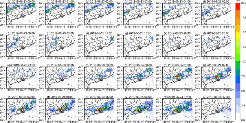
7008                                                             X. Li et al.: Leveraging machine learning for FY-4A QPE

remote-sensing spectral data have always been a challenging      tion estimation equation constructed with statistical methods
issue in satellite quantitative precipitation estimation (QPE)   (Atkinson and Tatnall, 1997). Machine learning is widely
(Lensky and Rosenfeld, 1995; Min et al., 2019).                  used in satellite QPE (Kühnlein et al., 2014; Min et al.,
   With the constant improvement of meteorological satel-        2019; Chen et al., 2019; Zhang et al., 2019; Sanò et al.,
lites, satellite-based QPE technology has developed greatly.     2015), and the random forest (RF) model is a modern
QPE satellite spectrum precipitation retrieval algorithms        machine-learning technique for classification and regres-
can be divided into visible/infrared (VIS/IR), microwave         sion, as well as a combined self-learning technique, which
and multi-combined spectral signals (Kidd, 2010; Leviz-          can easily capture the complex nonlinear relationship be-
zani et al., 2007). VIS/IR precipitation retrieval algorithms    tween observational and meteorological–environmental el-
mainly include the Geostationary Operational Environmen-         ements (Breiman, 2001; Bai et al., 2019a, b). It has been
tal Satellite (GOES) Precipitation Index algorithm (Arkin        widely applied to QPE. For instance, Kühnlein et al. (2014)
and Meisner, 2009), the GOES Multispectral Precipitation         divided data from the Spinning Enhanced Visible and In-
Algorithm (Ba and Gruber, 2001), the Griffith–Woodley al-        frared Imager carried onboard the Meteosat Second Gener-
gorithm (Griffith et al., 1978) and the Climate Estimation       ation satellite into day, dusk and nighttime to establish an
Centre Merged Analysis of Precipitation algorithm (Xie and       RF model and carry out QPE research, the results of which
Arkin, 2001). Rosenfeld and Gutman (1994) explored the           demonstrated a good effect on the estimation of rain area and
relationship between the effective radius of cloud retrieved     convective precipitation. Min et al. (2019) used Himawari-
by NOAA satellites and precipitation and proposed that an        8 real-time multi-band infrared brightness temperature and
effective radius greater than 14 µm should be the threshold      the Global Precipitation Measurement product to establish
for precipitation in the cloud. Previous studies have shown      a QPE method based on the RF model, from which it was
that different cloud microphysical parameters are closely        found that the accuracy of distinguishing the precipitation
related to the ground-level precipitation intensity, such as     area reached 0.87 and its average absolute error and mean
the substantially positive correlation between cloud optical     square error were 0.51 and 2.0 mm h−1 , respectively. Thus,
thickness/cloud liquid water content/cloud effective radius      there is strong evidence that the RF model can be applied
and the surface rain rate, while there is basically a nega-      effectively in precipitation monitoring and forecasting. The
tive correlation between the cloud-top temperature and sur-      Fengyun-4 satellite (FY-4A), launched in December 2016,
face rain rate (Fu, 2014; Nauss et al., 2008; Rosenfeld and      is China’s second-generation geostationary meteorological
Gutman, 1994; Rosenfeld et al., 2012; Yang et al., 2018).        satellite, and carried onboard is the Advanced Geostationary
Microwave precipitation retrieval algorithms include passive     Radiation Imager (AGRI) with 14 spectrum detection bands,
microwave (PMW) precipitation retrieval methods such as          covering the visible light, shortwave infrared, midwave in-
the Ferraro algorithm (Ferraro, 1997), Goda profile algo-        frared and longwave infrared bands. Thus far, QPE-based re-
rithm (Kummerow et al., 2001), and the Passive Microwave         search using FY-4A remains limited, especially in terms of
Neural Network Precipitation Retrieval approach for the EU-      the lack of an RF-based FY-4A QPE framework.
METSAT Satellite Application Facility on Support to Oper-           South China is one of the regions in the country with the
ational Hydrology and Water Management (H-SAF) (Mug-             longest rainy season, the most abundant precipitation and fre-
nai et al., 2013) as well as active precipitation retrieval      quent heavy rains. Affected by the westerly wind system and
methods based on the Precipitation Radar (PR) carried on-        the East Asian subtropical monsoon, the period from April to
board the Tropical Precipitation Measuring Mission satel-        June each year is the first rainy season (or the first flood sea-
lite (Iguchi et al., 2000) and the Global Precipitation Mea-     son) in South China. Therefore, it is important to strengthen
surement (GPM) Core Observatory spacecraft (Sharifi et al.,      the study of precipitation estimation and monitoring meth-
2016; Tan and Duan, 2017). Based on the higher temporal          ods in the first flood season in South China. In the present
sampling frequency of geostationary satellites, VIS/IR al-       work, taking South China (20–26◦ N, 109–118◦ E) as the re-
gorithms are suitable for retrieving continuous precipitation    search area, an RF algorithm model for FY-4A QPE is pro-
(Kidd, 2010), while PMW algorithms are better for retriev-       posed by using the spectral reflectance observations of FY-
ing instantaneous precipitation with higher accuracy (Ebert      4A/AGRI, meteorological environmental physical quantities
and Manton, 1996; Bauer et al., 1995), although PR also has      from the fifth major global reanalysis produced by the Euro-
the disadvantage of a limited observation range and uncertain    pean Centre for Medium-Range Weather Forecasts (ERA5)
parameters (Iguchi et al., 2009). Therefore, the development     and a precipitation dataset observed by a high-density auto-
of multi-spectral joint precipitation inversion algorithms can   matic station network with hourly resolution. The aims of
make up for the shortcomings of single-sensor algorithms         this study are to further improve the multi-spectral monitor-
(Michaelides et al., 2009; Holl et al., 2010).                   ing level of the FY-4A satellite and provide a scientific basis
   Because precipitation is a highly complex process, how-       for improving the disaster prevention and mitigation capabil-
ever, there is a nonlinear relationship between the sur-         ities of the FY-4A satellite.
face precipitation intensity and cloud-top optical physical
variables, resulting in certain limitations in the precipita-

Atmos. Meas. Tech., 14, 7007–7023, 2021                                           https://doi.org/10.5194/amt-14-7007-2021
X. Li et al.: Leveraging machine learning for FY-4A QPE 7009
2 Data and methods longitude and latitude of the maximum precipitation sta-
tion were 22.59◦ N, 111.04◦ E, and the precipitation in 48 h
2.1 Rainstorm cases was 149.3 mm. A central heavy-precipitation area covered
Guangzhou and its surrounding urban areas with high pop-
Rainstorms occurred frequently during the first flood sea- ulation density, where the distribution of automatic stations
son in South China in 2019, causing huge loss of life and is extremely dense. The longitude and latitude of the maxi-
property. We selected three rainstorms in South China dur- mum precipitation station were 23.28◦ N, 113.57◦ E, and the
ing 2019 that had a long period of precipitation with a large precipitation in 48 h was 220.5 mm. On the east side, a strong
coverage area. They are as follows: Case 1, 11–12 April 2019 precipitation centre formed in the southwest of Longyan City
(China standard time; if not specified, China standard time is and connected with Meizhou City to the west. The underly-
used); Case 2, 12–13 June 2019; Case 3, 23–24 June 2019. ing surface is mountainous, meaning that the distribution of
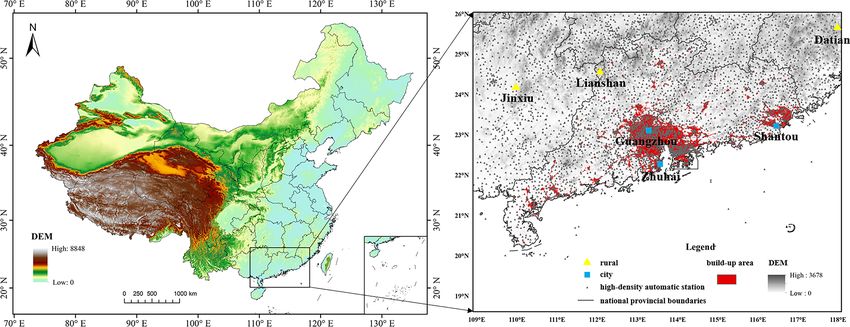
In addition to 215 national operated meteorological stations, automatic stations in this area is sparse. The longitude and
there are also 4706 automatic stations over the study re- latitude of the maximum precipitation station were 24.65◦ N,
gion, with a mean distance between them of less than 10 km 116.17◦ E, and the precipitation in 48 h was 239.4 mm. Three
(Fig. 1). Also, stations are deployed with higher density in strong rainfall areas obviously met the heavy-rain levels. The
the urban built-up area relative to the rural area. For the precipitation of 644 automatic stations exceeded 100 mm
high-density automatic station precipitation data in the range within 48 h, and the maximum precipitation was 239.4 mm
of 20–26◦ N and 109–118◦ E, after filtering and deleting the in the Haizhu District of Guangzhou (23.10◦ N, 113.30◦ E).
missing and mis-detected data, the number of automatic sta- Among the three cases, Case 1 had a small distribution of
tions for the three cases was 4263, 4610 and 4623, respec- heavy precipitation, and the accumulated precipitation was
tively. The distribution of high-density automatic stations the smallest among the three cases. Case 2 had 29 stations
throughout the country and in the research area is shown with a 48 h accumulated precipitation exceeding 200 mm and
in Fig. 1, and the spatial distributions of precipitation dur- with more extreme heavy precipitation. Case 3 had the largest
ing the three South China rainstorms are shown in Fig. 2. number of stations meeting the rainstorm level and had a
The red shading in Fig. 1 shows the built-up area in South wide distribution. The types of underlying surface covered by
China, which was extracted using nighttime light (NTL) data the precipitation were diverse, and the centre of the rainstorm
obtained by the Visible Infrared Imaging Radiometer Suite was located in the central urban agglomeration and densely
(VIIRS) on board the Suomi National Polar Orbiting Part- populated areas, which meant that the threat to human life
nership (NPP) satellite. In Case 1 (Fig. 2a), large-scale heavy and property was high, so Case 3 is more typical and rep-
precipitation mainly occurred in the southern coastal area of resentative and can serve as a case study for the other two
Guangdong Province. From north to south, there were three cases. This paper therefore takes the heavy-rain process of
bands of precipitation extremes, and the accumulated precip- 23–24 June as an example to discuss the QPE method of FY-
itation gradually decreased from southwest to northeast. In 4A based on the RF model and physical quantities. The esti-
total, 159 automatic stations recorded precipitation exceed- mation and validation results of the RF model for Case 1 and
ing 100 mm within 48 h, and the maximum precipitation in Case 2 are provided in the Supplement.
Jiujiang Town, Foshan City (22.83◦ N, 112.99◦ E), on the or-
der of 192 mm, reached rainstorm levels. (The specific rain- 2.2 Data
fall classification of is supplied in Table S1 in the Supple-
ment.) The 14 bands of FY-4A/AGRI have different detection pur-
In Case 2 (Fig. 2b), there was a belt of accumulated heavy poses and can identify different spectral characteristics of
precipitation in the northwest mountainous area and a large different surfaces, clouds or atmospheres (Table S2 in the
area of heavy precipitation in the northeast of the central ur- Supplement). FY4A/AGRI takes about 15 min to perform a
ban area. The 48 h automatic station precipitation amounts full-disk image observation and has a maximum spatial reso-
in these two concentrated heavy-precipitation areas both ex- lution of 500 m. FY4A/AGRI provides a level-1 dataset with
ceeded 100 mm, which meant that the precipitation intensity resolutions of 500 m and 1, 2 and 4 km at nadir. For the level-
met the heavy-rain level (see Table S1, also regarding the fol- 2 dataset, it provides a resolution of 4 km at nadir. These
lowing description of precipitation level). The precipitation values meet the requirements for the spatial and temporal
of 492 automatic stations exceeded 100 mm within 48 h, and resolution of satellite monitoring of rainstorms. In order to
the maximum precipitation was 318.7 mm in Fogang County, train the RF model, we used the FY-4A/AGRI full-disk data
Qingyuan City (23.91◦ N, 113.93◦ E). with a temporal resolution of 1 h and spatial resolution of
In Case 3 (Fig. 2c), there were three heavy-precipitation 4 km×4 km during the study period, which contains 14 bands
areas that met the heavy-rain level. The heavy-precipitation of radiation brightness temperature and reflectance informa-
area on the west side extended from Yulin City to the tion. At the same time, the combined channel information
southeast to the north of Maoming City. The distribution of was constructed based on the level-1 data.
high-density automatic stations in this area is sparse. The
https://doi.org/10.5194/amt-14-7007-2021 Atmos. Meas. Tech., 14, 7007–7023, 2021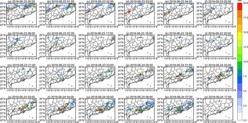
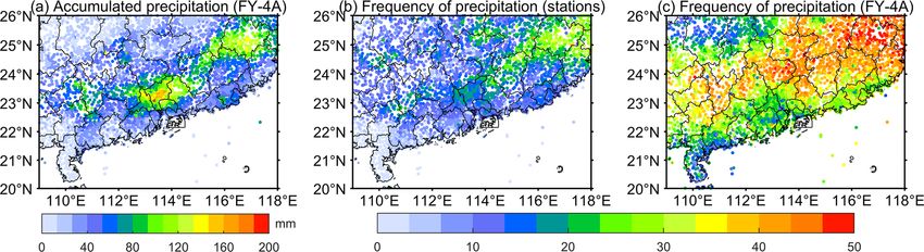
7010                                                                    X. Li et al.: Leveraging machine learning for FY-4A QPE

Figure 1. Distribution of automatically operated meteorological stations over the study area.

Figure 2. Spatial distribution of precipitation during the three South China rainstorms: (a) 11–12 April 2019; (b) 12–13 June 2019; (c) 23–
24 June 2019.

   Due to the indirect link between the surface rain rate and            and multi-layer ice. CLT and CLP are commonly used to de-
the cloud-top brightness temperature (Thies et al., 2008),               tect and track changes in water vapour composition in clouds
the inversion accuracy is limited. To ensure the stability of            and extreme weather estimation to improve extreme weather
training and estimation as well as improve the estimation                warning capabilities.
accuracy, according to existing research (Kühnlein et al.,                  In addition to the FY-4A/AGRI observation data, this pa-
2014; Min et al., 2019), four level-2 cloud parameter prod-              per also uses physical quantities from ERA5 to further im-
ucts (cloud-top temperature (CTT), cloud-top height (CTH),               prove the performance of the QPE algorithm. These data
cloud type (CLT) and cloud phase (CLP)) observed in real                 have a horizontal resolution of 0.25◦ × 0.25◦ , a vertical res-
time from FY-4A were selected. For each cloud parameter                  olution of 37 layers and a temporal resolution of up to
product, the temporal resolution is 1 h and the spatial resolu-          1 h. ERA5 is widely used in the study of weather and cli-
tion 4 km × 4 km, which is consistent with the level-1 data.             mate change. According to previous studies (Min et al.,
CTT and CTH are the cloud-top temperature and height in-                 2019; Kanamitsu, 1989), we introduce some ERA5 re-
formation of cloud pixels obtained by the inversion of AGRI              analysis data to further and better support QPE, includ-
infrared channel data, which can be used to determine the                ing six physical weather indexes, which can effectively de-
likelihood of cloud growth, extinction and precipitation. CLT            scribe the atmospheric heat (K index), dynamics (convective
is four different cloud phases generated from AGRI infrared              available potential energy (CAPE); eastward turbulent sur-
channel data – namely, warm liquid water (> 0◦ ), super-                 face stress (EWSS)), humidity (total column water vapour
cooled liquid water, mixed phase and ice phase. CLP uses                 (TCWV); total column water (TCW)) and topographic fea-
data from multiple infrared channels of AGRI to obtain six               tures (anisotropy of sub-gridscale orography (ISOR)). These
different cloud types through a series of spectral and spa-              indexes are closely associated with the initiation and devel-
tial tests: water, supercooled water, mixed, thick ice, thin ice         opment of clouds that produce rain (Zhang, 2003; Roman

Atmos. Meas. Tech., 14, 7007–7023, 2021                                                    https://doi.org/10.5194/amt-14-7007-2021
X. Li et al.: Leveraging machine learning for FY-4A QPE                                                                       7011

et al., 2016). In order to improve the generalisation ability       weather station to match the in situ precipitation measure-
of the algorithm precipitation estimation and solve the differ-     ment and satellite data at each pixel.
ence of algorithm precipitation estimation in plain and moun-          Ten indicators are defined to judge the accuracy of the
tain areas, this paper introduces the digital elevation model       QPE algorithm (Table 2). In order to quantitatively eval-
(DEM) as one of the input variables. It is the digital expres-      uate the classification results of precipitation and non-
sion of surface morphology and contains rich topographic            precipitation pixels, we introduce eight classical metrics:
and geomorphic information.                                         bias score (Bias, Bias = 1 unbiased, Bias < 1 underesti-
                                                                    mation, Bias > 1 overestimation), probability of detection
2.3   RF model design                                               (POD, optimal = 1), false alarm ratio (FAR, optimal = 0), ac-
                                                                    curacy (ACC, optimal = 1), Critical Success Index (CSI, op-
A data-driven regression model was established between the          timal = 1), Heidke Skill Score (HSS, optimal = 1), Hanssen
observed precipitation and satellite data as well as cloud pa-      and Kuiper (HK, optimal = 1), and Equitable Threat Score
rameters using the RF method. The essence of the RF data            (ETS, optimal = 1). Among them, when POD or FAR take
estimation model is as follows.                                     the optimal value, the algorithm cannot be determined as
   The input variables to the RF model are shown in Ta-             the optimal estimation. When ACC or CSI take the optimal
ble 1, including geographic information, channel informa-           value, the algorithm can be determined as the optimal esti-
tion, combined channel information, cloud parameter prod-           mation. HSS, HK and ETS are all commonly used to evalu-
ucts and ERA5 data. A daytime quantitative precipitation es-        ate the estimating ability of algorithms as skill scores. HSS
timate (DQPE) algorithm and a nighttime quantitative pre-           compares the accuracy between the algorithm and a random
cipitation estimate (NQPE) algorithm were constructed sep-          estimation as reference by the accuracy score ACC, and ETS
arately, due to different input variables between daytime and       compares the accuracy between the algorithm and another
nighttime. The DQPE algorithm is used to estimate the pre-          random estimation as reference by the accuracy score CSI.
cipitation from 08:00 to 16:00, and the NQPE algorithm is           When HSS > 0 or ETS > 0, the algorithm is skilful and its
used to estimate the remaining time periods. The visible light      estimation ability is better than random estimation as ref-
channel at nighttime cannot produce valid observational in-         erence. HK is defined as the difference between POD and
formation, so the NQPE algorithm removes these variables.           probability of false detection (POFD). When HK > 0, the al-
The CTT gradient (CTTG ) in the combined channel infor-             gorithm is skilful, and when HK = HSS, the algorithm gives
mation is closely related to the rain rate, defined as follows      an unbiased estimation. There are two other indicators that
Eq. (1):                                                            can be used to quantitatively evaluate the accuracy of pre-
                                                                    cipitation estimation based on the QPE algorithm. They are
                                                                    the correlation coefficient (R, optimal = 1) and root-mean-
          n                             2
CTTG =      T (i + 1, j ) − T (i − 1, j )
                                                                    square error (RMSE, optimal = 0).
                                      2 o 21                         The establishment of the RF model needs to determine two
          + T (i, j + 1) − T (i, j − 1)        ,             (1)    important parameters – namely, the number of input variables
                                                                    of tree nodes, mtry, and the number of decision trees, ntree.
where T represents the spectral brightness temperature of           Besides, the larger the mtry, the smaller the overfitting effect
10.7 µm and i and j represent the pixel position.                   of the RF algorithm; while the larger the ntree, the smaller the
   We selected the 1 h temporal resolution high-density auto-       difference between the submodels. The value of mtry should
matic station geographic and precipitation information, satel-      be smaller than the value √ of the input variable. In general,
lite observation data, and ERA5 reanalysis data to input into       mtry values are 1, k/2, 2 k and log2 (k) + 1, etc., where k is
the QPE algorithm for precipitation estimation. The spatial         the number of variables input into the model. We selected
resolution of FY-4A/AGRI is 4 km × 4 km, the spatial resolu-        k/2 as the number of input variables of the tree node; that
tion of ERA5 is 0.25◦ × 0.25◦ , and the spatial resolution of       is, mtry = 17. The number of decision trees, ntree, is ideally
DEM is 1 km × 1 km. Due to this difference in spatial resolu-       classified when the value of ntree is between 500 and 800.
tion, the above-mentioned data needed to be interpolated to         We set it to 550.
construct a dataset that was synchronised in time and space.           We randomly created mtry pieces of variables for the bi-
According to a previous study (Liu et al., 2020), the differ-       nary tree on the node, and the choice of the binary tree vari-
ences between a diverse interpolation methods are small for         ables still meets the principle of minimum node impurity.
high-density automatic stations, with the effect of interpola-      The bootstrap self-help method is applied to randomly select
tion depending mainly on the station distribution rather than       ntree sample sets from the original dataset to form a decision
the interpolation method itself. In this paper, for matching        tree of ntree, and the unsampled samples are used for the
input variables with precipitation data, we employed spline         estimation of a single decision tree. Samples are classified
interpolation on the satellite data to match the in situ precipi-   or predicted according to the RF composed of ntree decision
tation measurement, while we used the averaged value of the         trees. The principle of classification is the voting method, and
four nearest grids of ERA5 data and DEM data around each            the principle of estimation is the simple average.

https://doi.org/10.5194/amt-14-7007-2021                                              Atmos. Meas. Tech., 14, 7007–7023, 2021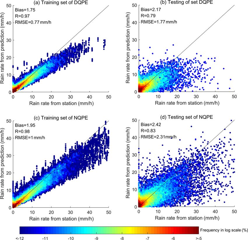
7012                                                                                            X. Li et al.: Leveraging machine learning for FY-4A QPE

Table 1. Variables used in the QPE algorithm.

                                                   Variables
     Geographic information                        Longitude, latitude, DEM
     Channel information of AGRI                   T0.47∗ , T0.65∗ , T0.825∗ , T1.375∗ , T1.61∗ , T2.25∗ , T3.75H, T3.75L, T6.25, T7.1, T8.5, T10.7,
                                                   T12.0, T13.5
     Combined information of AGRI                  T6.25–T10.7, T8.5–T10.7, T7.1–T12.0, T12.0–T10.7, T3.75L–T7.1, T3.75L–T10.7, CTTG
     Cloud parameters of AGRI                      CTT, CTH, CLT, CLP
     ERA5                                          ISOR, CAPE, EWSS, K index, TCW, TCWV

   Notation: asterisk (∗ ) indicates that the variable does not appear in the NQPE algorithm.

Table 2. Evaluation metrics used in this study.

                                    Evaluation metric           Equation

                                    Bias                        Bias = A+B
                                                                       A+C

                                    POD                                A
                                                                POD = A+C

                                    FAR                                B
                                                                FAR = A+B

                                    ACC                                 A+D
                                                                ACC = A+B+C+D

                                    CSI                                 A
                                                                CSI = A+B+C

                                    HSS                         HSS = ACC−A  ref1
                                                                       1−Aref1 , Aref1 =
                                                                                         (A+B)(A+C)+(C+D)(B+D)
                                                                                                A+B+C+D

                                    HK                                              AD−BC , POFD = B
                                                                HK = POD − POFD = (A+C)(B+D)      B+D
                                                                                Aref2
                                                                          CSI− A+B+C          A−Aref2
                                    ETS                         ETS =          Aref2  = A+B+C−A            ,        Aref2 = (A+B)(A+C)
                                                                                                                             A+B+C+D
                                                                          1− A+B+C                    ref2
                                                                         Pn
                                                                              (G −Ḡ)(S −S̄)
                                    R                           R=     Pn i=1 i Pn i
                                                                        i=1 (Gi −Ḡ) i=1 (Si −S̄)
                                                                             s
                                                                                    n
                                    RMSE                        RMSE =           1 P (G − S )2
                                                                                 n     i   i
                                                                                   i=1

                                  Notation: A is the number of imagery pixels identified by both the stations and the QPE algorithm as
                                  precipitation; B is the number of imagery pixels identified by the QPE algorithm as precipitation but not by
                                  the stations; C is the number of imagery pixels identified by the stations as precipitation but not by the QPE
                                  algorithm; D is the number of imagery pixels identified by both the stations and the QPE algorithm as
                                  non-precipitation. Gi is the precipitation observed by stations; Si represents the precipitation estimated by the
                                  QPE algorithm.

   Finally, Fig. 3 summarises the flowchart for the QPE al-                                     was judged as a precipitation pixel; otherwise, it was judged
gorithm using the RF model. According to previous stud-                                         as a non-precipitation pixel.
ies (Yang et al., 2020; Zeng et al., 2020), a 10-fold cross-
validation (10-fold CV) method was used to test the model
estimation performance. The 10-fold CV method makes                                             3     Results
maximum use of the existing sample data and ensures that
each sample is used as a training sample and a test sample, re-                                 3.1    RF model evaluation
spectively, effectively avoiding the result of overfitting. The
training set was input into the RF model, and the QPE algo-                                     This paper uses 10-fold CV to evaluate the accuracy of pre-
rithm with the highest estimation accuracy was constructed                                      cipitation estimation. Figure 4 compares the precipitation ob-
by performing 10-fold CV. The testing set was input into the                                    servations of the high-density automatic stations in the train-
RF model to obtain the precipitation estimation of each pixel                                   ing set and the testing set with the precipitation estimation of
and judge whether the pixel was a precipitation pixel. For a                                    the QPE algorithm in the 10-fold CV of the DQPE algorithm
pixel with precipitation intensity greater than 0.1 mm h−1 , it                                 and the NQPE algorithm, in which the colour bar represents
                                                                                                the occurrence frequency on a log scale with an interval of

Atmos. Meas. Tech., 14, 7007–7023, 2021                                                                               https://doi.org/10.5194/amt-14-7007-2021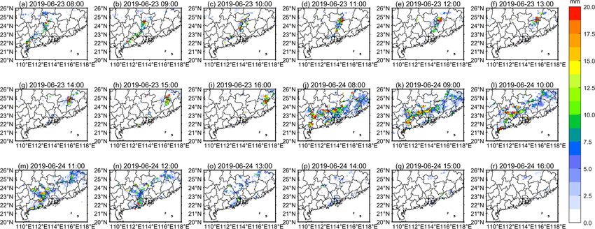
X. Li et al.: Leveraging machine learning for FY-4A QPE                                                                       7013

Figure 3. Flowchart for the QPE algorithm using the RF model.

0.5 mm h−1 . In the training set, the Bias, R and RMSE of the          Table 3 shows the evaluation metrics in a training set and
DQPE (NQPE) algorithm are 1.75 (1.95), 0.97 (0.98) and              a testing set of the DQPE (NQPE) algorithm. The POD of
0.77 mm h−1 (1.00 mm h−1 ), respectively. In the testing set,       the QPE algorithm is 0.98 and above, and the FAR is around
the Bias, R and RMSE of the DQPE (NQPE) algorithm are               0.5. As to the precipitation pixels, the QPE algorithm can
2.17 (2.42), 0.79 (0.83) and 1.77 mm h−1 (2.31 mm h−1 ), re-        accurately identify them; but for the precipitation pixels es-
spectively. For the heavy-rain level and below precipitation        timated by the QPE algorithm, the probability that the pixel
observation samples, the large amount of precipitation obser-       has precipitation is about 50 %. The ACC reaches 0.6 and
vations and estimations are close to the 1 : 1 line. It reflects    above, indicating that for more than 60 % of the data sam-
that the algorithm has a high quantitative estimation ability       ples, the QPE algorithm can accurately distinguish between
for precipitation of heavy-rain level and below. Bias values        precipitation and non-precipitation pixels. The CSI is 0.4 and
are all greater than 1, reflecting that the QPE algorithm tends     above, which means that the accurately estimated precipita-
to overestimate precipitation events. The feature of the al-        tion pixel samples account for more than 40 % of all observed
gorithm overestimating precipitation events is mainly mani-         and estimated precipitation pixel samples. HK reflects the
fested in weak precipitation and non-precipitation pixels. For      difference between POD and the probability of false detec-
example, there are obviously a large number of observation          tion (POFD). The HK of the QPE algorithm is around 0.5 and
sample points without precipitation in Fig. 4, and their pre-       above, indicating that the proportions of correct estimations
cipitation estimation is too high. When the precipitation ob-       in all precipitation pixels are far greater than the proportions
servations reach the rainstorm level and above, the QPE al-         of incorrect estimations in all non-precipitation pixels. HSS
gorithm tends to underestimate the precipitation. This kind of      (ETS) reaches 0.3 and above (0.2 and above), reflecting that
estimation error can be reduced by secondary training. In ad-       the QPE algorithm is skilful and better than random estima-
dition, it is found that there exists a notable difference in the   tion as a reference (Aref1 and Aref2 in Table 2). The evalua-
performance between testing and training for the QPE algo-          tion metrics of the QPE algorithm for Case 1 and Case 2 are
rithm. This gap is suspected to be caused by overfitting that       shown in Table S2 in the Supplement.
is possibly related to the high complexity of the RF model
(Lao et al., 2021). The effect of the QPE algorithm on Case 1
and Case 2 is shown in Fig. S1 in the Supplement.

https://doi.org/10.5194/amt-14-7007-2021                                              Atmos. Meas. Tech., 14, 7007–7023, 2021
7014 X. Li et al.: Leveraging machine learning for FY-4A QPE
Figure 4. Comparison of the precipitation measured by high-density automatic stations and that estimated by the QPE algorithm: (a) training
set of DQPE; (b) testing set of DQPE; (c) training set of NQPE; (d) testing set of NQPE. Colour bar: occurrence frequency (on a log scale)
at intervals of 0.5 mm h−1 .
Table 3. Evaluation metrics in training set and testing set of DQPE (NQPE) algorithm.
Model name POD FAR ACC CSI HSS HK ETS
Training set of DQPE 1.00 0.43 0.78 0.57 0.57 0.69 0.39
Testing set of DQPE 0.98 0.55 0.65 0.45 0.37 0.50 0.23
Training set of NQPE 1.00 0.49 0.76 0.51 0.51 0.67 0.35
Testing set of NQPE 0.98 0.59 0.63 0.40 0.33 0.49 0.20
3.2 Application of the RF model to QPE cation and range of extreme precipitation pixels but cannot
accurately and quantitatively estimate extreme precipitation.
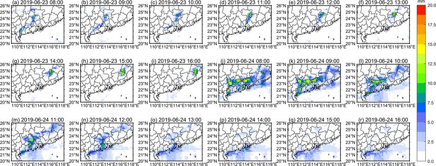
Figure 5 shows the hourly precipitation distribution as esti- This is similar to the results of previous studies (Kühnlein
mated by the DQPE algorithm, and Fig. 6 shows the actual et al., 2014; Min et al., 2019). At 11:00–16:00 on 24 June, the
precipitation observations at high-density automatic stations precipitation centre gradually moved to the sea surface. Due
in the daytime, with a temporal resolution of 1 h. Compari- to the lack of geographic information provided by the high-
son of Figs. 5 and 6 shows that the precipitation estimation density automatic stations for training at the sea surface, the
of the DQPE algorithm is consistent with the actual precip- accuracy of the estimation is low. However, for land-surface
itation observations at high-density automatic stations, and precipitation, the size, location and coverage of the precipi-
the DQPE algorithm can capture the precipitation range well. tation estimated by the DQPE algorithm is highly consistent
However, when the precipitation exceeds 20 mm h−1 , the with the actual precipitation observations. The precipitation
algorithm obviously underestimates the precipitation. This estimation in Case 1 and Case 2 by the DQPE algorithm is
means that the algorithm can only roughly estimate the lo- shown in Fig. S2 in the Supplement. The distribution of the
Atmos. Meas. Tech., 14, 7007–7023, 2021 https://doi.org/10.5194/amt-14-7007-2021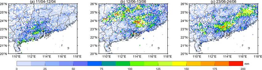
X. Li et al.: Leveraging machine learning for FY-4A QPE 7015
measured precipitation in the daytime from the high-density is relatively greater and vice versa in the southwest. The pre-
automatic stations in Case 1 and Case 2 is shown in Fig. S3 cipitation frequency estimated by the QPE algorithm is gen-
in the Supplement. erally greater than observed. This is because there are more
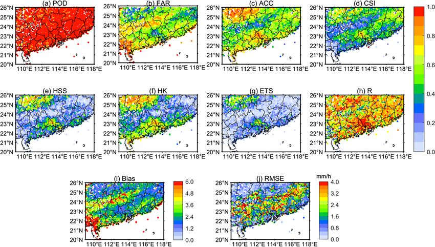
Figure 7 shows the hourly distribution of precipitation as non-precipitation events for most stations and the algorithm
estimated by the NQPE algorithm, and Fig. 8 shows the ac- often incorrectly judges non-precipitation areas as weak pre-
tual precipitation observed at the high-density automatic sta- cipitation stations as Bias is greater than 1, resulting in a pos-
tions at nighttime. Comparing Figs. 7 and 8, a conclusion itive bias in the precipitation frequency estimated by the QPE
similar to that from the DQPE algorithm can be obtained. algorithm at each station. The spatial distribution of accumu-
The precipitation estimation of Case 1 and Case 2 by the lated precipitation in Case 1 and Case 2 is shown in Fig. S6
NQPE algorithm is shown in Fig. S4 in the Supplement. in the Supplement.
The distribution of precipitation at nighttime observed by Figure 11 shows the spatial distribution of evaluation indi-
the high-density automatic stations in Case 1 and Case 2 is cators of the QPE algorithm for all stations. Except that the
shown in Fig. S5 in the Supplement. In general, the estima- POD of almost all stations is close to 1 in Fig. 11a, the spatial
tion ability of the QPE algorithm is strong over the land sur- distribution of the rest of the evaluation indicators has obvi-
face. This proves the applicability and feasibility of estab- ous correlation. In Fig. 11b and i, the spatial distribution of
lishing an RF model and training the QPE algorithm based FAR and Bias has a significant negative correlation with ac-
on the model variables in Table 1. cumulated precipitation. FAR is often lower and Bias tends
to 1 in areas with more accumulated precipitation, such as
3.3 Verification of the QPE the three heavy-precipitation centres in the precipitation pro-
cess mentioned above. By contrast, the FAR and Bias are
In order to further analyse the factors that affect the esti- higher in areas with less accumulated precipitation, such as
mation accuracy of the QPE algorithm, we selected three the southwest coastal area. According to the FAR and Bias
city stations as research targets: Guangzhou (23.13◦ N, calculation formula (Table 2), this reduces the FAR and Bias
113.30◦ E), Shantou (23.38◦ N, 116.50◦ E) and Zhuhai by increasing the number of precipitation pixels detected by
(22.28◦ N, 113.57◦ E). At the same time, we selected both stations and the QPE algorithm. There is a low-FAR
three rural stations as research targets: Datian (25.80◦ N, and low-Bias zone in the mountainous area in the northwest
117.93◦ E), Lianshan (24.63◦ N, 112.03◦ E) and Jinxiu of the study area, which does not have the above character-
(24.09◦ N, 109.99◦ E). Figure 9 shows the actual precipita- istics. Combined with the results shown in Fig. 8a–h, we can
tion observations of these six stations and the accumulated see that there has been weak precipitation in the area for at
precipitation estimated by the QPE algorithm for 48 consec- least 8 consecutive hours. According to the FAR and Bias
utive hours. Based on the precipitation observations and esti- calculation formula (Table 2), this reduces the FAR by re-
mations at each time of 48 h, we used Bias, R and RMSE to ducing the number of precipitation pixels that are not de-
evaluate the ability of the algorithm for precipitation estima- tected by the stations but are detected by the QPE algorithm.
tion. For the six research sites, Bias values are all greater than Therefore, FAR and Bias are negatively correlated with pre-
1, reflecting that the algorithm tends to overestimate precipi- cipitation intensity and duration. When the precipitation in-
tation events, which is consistent with the conclusion above. tensity is greater and the duration is longer, the FAR of the
Based on R and RMSE, there is no obvious difference be- QPE algorithm is lower, the Bias gets closer to 1, and the de-
tween city sites and rural sites. The time and size of the cu- viation by which the QPE algorithm accurately distinguishes
mulative precipitation changes in the six research sites are between precipitation and non-precipitation pixels is smaller.
almost the same, reflecting that the algorithm has a strong The spatial distribution of ACC, CSI, HSS, HK and ETS
quantitative estimation ability and does not change with city has an obvious positive correlation with accumulated precip-
and rural areas. We may think that the precipitation estima- itation. According to Fig. 11c and d, the QPE algorithm cor-
tion ability of the algorithm is less affected by the difference rectly estimated that the precipitation pixels accounted for
between city and rural areas. a relatively high proportion in the three heavy-precipitation
Figure 10a presents the 48 h accumulated precipitation es- centres and the northwest mountainous area, indicating that
timated by the QPE algorithm. Compared with Fig. 2c, all for heavy convective precipitation and long-lasting strati-
three heavy-precipitation centres are estimated, and the area graphic clouds precipitation, the QPE algorithm’s ability
and intensity in the precipitation estimations and in the ac- to accurately distinguish between precipitation and non-
tual observations are basically the same. It shows that the precipitation pixels is stronger. The higher value positions
algorithm has strong potential in accurately estimating the in Fig. 11e, f and g are basically the same as Fig. 11c and d.
intensity and range of precipitation. Figure 10b and c, re- However, for areas with heavy precipitation in the northeast,
spectively, represent the actual precipitation frequency ob- the values of HSS, HK and ETS are relatively low. This is be-
served by the high-density automatic stations and that esti- cause the heavy-precipitation area in the northeast has higher
mated by the QPE algorithm. The results indicate that the precipitation frequency during the study period (Fig. 10b),
frequency of precipitation in the northeast of the study area which makes the random estimation improve the probabil-
https://doi.org/10.5194/amt-14-7007-2021 Atmos. Meas. Tech., 14, 7007–7023, 2021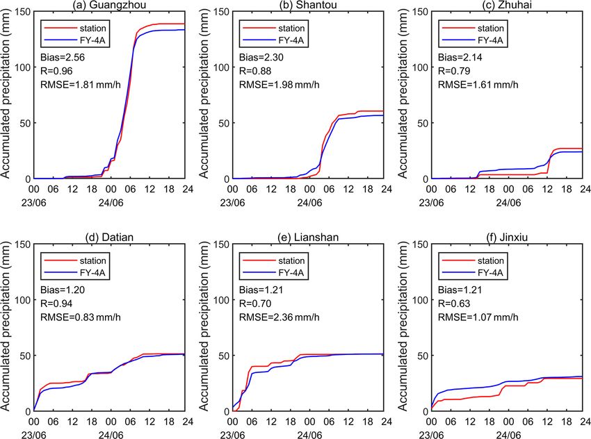
7016                                                                  X. Li et al.: Leveraging machine learning for FY-4A QPE

Figure 5. Estimated precipitation of the DQPE algorithm at (a–i) 08:00–16:00 CST on 23 June and (j–r) 08:00–16:00 CST on 24 June.

Figure 6. Actual precipitation based on high-density automatic stations at (a–i) 08:00–16:00 CST on 23 June and (j–r) 08:00–16:00 CST on
24 June.

ity of accurately estimating the precipitation pixels. Then the       counting for 14.41 %. Comparing Fig. 11b to g, the stations
advantage of ACC and CSI over random estimation will be               with lower R have relatively higher FAR and Bias and lower
weakened, and this results in low HSS and ETS values. The             ACC, CSI, HSS, HK and ETS. The 48 h accumulated precip-
higher precipitation frequency in the northeast leads to a de-        itation of these stations is less than 12.5 mm, and the accu-
crease in the number of imagery pixels identified by both             mulated precipitation is less than 5 h. This basically means
the stations and the QPE algorithm as non-precipitation. This         that, during this precipitation process, these stations are in
results in high POFD values. When the POD remains un-                 atypical stratus cloud or a convective precipitation process,
changed (Fig. 11a), the value of HK decreases. Comparing              and the precipitation efficiency is extremely low. For non-
Fig. 11e and f, the heavy-precipitation area in the northeast         precipitation areas in a heavy-precipitation process, the QPE
basically satisfies HSS = HK, which means that the algo-              algorithm tends to judge them as weak precipitation areas,
rithm in the northeast is an unbiased estimation. In summary,         this shows that the algorithm overestimations the precipita-
although the values of HSS, HK and ETS in the northeast are           tion areas. Although the QPE algorithm tends to overesti-
relatively low, the algorithm still has a high ability to distin-     mate the weak (non-) precipitation area and underestimate
guish between precipitation and non-precipitation pixels.             the heavy-precipitation area, the absolute error for the under-
   For Fig. 11h, there are 2660 stations with R > 0.8, ac-            estimated heavy-precipitation area is much larger than the
counting for 59.45 %, and 600 stations with R < 0.6, ac-              overestimated weak (non-) precipitation area. Therefore, the

Atmos. Meas. Tech., 14, 7007–7023, 2021                                                 https://doi.org/10.5194/amt-14-7007-2021
X. Li et al.: Leveraging machine learning for FY-4A QPE                                                                        7017

Figure 7. Estimated precipitation of the NQPE algorithm at (a–h) 00:00–07:00 CST on 23 June, (i–o) 17:00–23:00 CST on 23 June, (p–
w) 00:00–07:00 CST on 24 June and (x) 17:00 CST on 24 June.

Figure 8. Actual precipitation based on high-density automatic stations at (a–h) 00:00–07:00 CST on 23 June, (i–o) 17:00–23:00 CST on
23 June, (p–w) 00:00-07:00 CST on 24 June and (x) 17:00 CST on 24 June.

spatial distribution of RMSE in Fig. 11j is highly consis-           the stations with a 48 h accumulated precipitation exceeding
tent with the spatial distribution of 48 h accumulated precip-       50 mm h−1 in Fig. 2c.
itation in Fig. 2c. The stations with an RMSE greater than              In summary, the estimating ability of the QPE algorithm
1.6 mm h−1 in Fig. 11j are basically connected together, and         is as follows: (1) for convective precipitation or stratus con-
their coverage is basically the same as the area covered by          vective mixed precipitation with long duration, high inten-
                                                                     sity and high efficiency, such as in Guangzhou and nearby

https://doi.org/10.5194/amt-14-7007-2021                                               Atmos. Meas. Tech., 14, 7007–7023, 2021
7018 X. Li et al.: Leveraging machine learning for FY-4A QPE Figure 9. Accumulated precipitation in different areas: (a–c) city stations; (d–f) rural stations. Figure 10. Spatial distribution of accumulated precipitation: (a) accumulated precipitation estimated by the QPE algorithm; (b) actual precipitation frequency observed by high-density automatic stations; (c) precipitation frequency estimated by the QPE algorithm. urban areas in Case 3, the algorithm has high POD, ACC, CSI, HSS, HK, ETS and R are relatively low, and the relia- CSI, HSS, HK and ETS, low FAR, and R and Bias close bility of the estimating ability of the QPE algorithm is low. to 1. The RMSE of such precipitation events is affected by For Case 1 and Case 2, the hourly spatial distribution of eval- the precipitation intensity. In this precipitation process, the uation indicators for both QPE algorithms at each station is QPE algorithm has the strongest estimating ability. (2) For shown in Fig. S7 in the Supplement. precipitation with long duration and weak intensity per unit Figure 12 shows the time series of evaluation indicators of time, such as in the northwest mountainous area in Case 3, the QPE algorithm for all stations at each time. The red lines the POD, FAR, ACC, CSI, HSS, HK and ETS of the algo- represent the average values of the evaluation indicators, rithm show roughly the same characteristics as the previous from which we can see that the average values of POD, FAR, type of precipitation. The R also declines slightly but is still ACC, CSI, HSS, HK, ETS, R, Bias and RMSE are 0.97, 0.60, near 0.8. The RMSE is greatly reduced. The estimating abil- 0.64, 0.40, 0.31, 0.47, 0.19, 0.70, 2.87 and 1.90 mm h−1 , re- ity of the QPE algorithm is second to the previous precipita- spectively. From 01:00 to 14:00 on 24 June, the POD, ACC, tion process. (3) When the duration of precipitation is short CSI, HSS, HK, ETS, R and RMSE are high, the FAR is low, and the intensity is only light to moderate rain, such as in and the Bias tends to 1. According to Figs. 6j–p and 8q–w, the southwest coastal area in Case 3, the FAR and Bias es- the intensity of the precipitation centre during this period ex- timated by the QPE algorithm are relatively high, the ACC, ceeds 16 mm h−1 , reaching rainstorm level. At this point, the Atmos. Meas. Tech., 14, 7007–7023, 2021 https://doi.org/10.5194/amt-14-7007-2021
X. Li et al.: Leveraging machine learning for FY-4A QPE                                                                               7019

Figure 11. Spatial distribution of evaluation indicators of the QPE algorithm for all stations: (a) POD; (b) FAR; (c) ACC; (d) CSI; (e) HSS;
(f) HK; (g) ETS; (h) R; (i) Bias; (j) RMSE.

Figure 12. Time series of evaluation indicators of the QPE algorithm for all stations at each time: (a) POD; (b) FAR; (c) ACC; (d) CSI;
(e) HSS; (f) HK; (g) ETS; (h) R; (i) Bias; (j) RMSE.

estimation accuracy of the QPE algorithm is strong. Not only            comparing Fig. 5 with Figs. 6j–l and 7 with Fig. 8q–w. This
is the effect of the evaluation indicator good, but also the in-        proves that, for the strong convective process with a short
tensity of the precipitation centre and the precipitation range         precipitation duration and the precipitation intensity reach-
of these periods fit with a high accuracy, as can be seen by            ing rainstorm level, the evaluation indicators show similar

https://doi.org/10.5194/amt-14-7007-2021                                                   Atmos. Meas. Tech., 14, 7007–7023, 2021
7020                                                               X. Li et al.: Leveraging machine learning for FY-4A QPE

characteristics to the first type of precipitation above. At the   implying that when the rain rate is large enough (rainstorm
same time, this means that when the precipitation intensity        level or above), the precipitation duration is no longer a fac-
is large enough, the precipitation duration is no longer the       tor affecting the accuracy of the QPE algorithm. (2) For pre-
main factor influencing the estimating ability of the QPE al-      cipitation processes with a long duration at a low rain rate,
gorithm. At 00:00–04:00 on 23 June, the POD, ACC, CSI,             the algorithm shows a roughly similar accuracy as the pre-
HSS, HK, ETS, R and RMSE are higher than their average             vious type of precipitation but with a slight degradation in
values, while the FAR and Bias are lower than their average        R, whereas there is a significant increase in RMSE. (3) For
values. The characteristics of each evaluation indicator dur-      precipitation with a short duration at a small to moderate in-
ing this period are similar to the second type of precipitation    tensity, the QPE algorithm showed a relatively high FAR and
above. Comparing Fig. 7 with Fig. 8a–d, the precipitation in-      Bias but a relatively low ACC, CSI, HSS, HK, ETS and R,
tensity and range are basically successfully fitted, but the es-   implying a low accuracy of the QPE algorithm.
timation of precipitation in localised areas is not good. This        In general, by synergistically using high-density automatic
verifies the previous conclusion that the QPE algorithm’s es-      station data and meteorological physical quantity fields, the
timating ability for long-duration and weak-intensity precip-      QPE algorithm developed in this study provides a promis-
itation is inferior to that of strong convective precipitation.    ing way for quantitative estimation of summer precipitation
From 17:00 to 20:00 on 23 June, the POD, ACC, CSI, HSS,            over East Asia from FY-4A satellite observations. Our re-
HK, ETS, R and RMSE are all lower than their average val-          sults also highlight the beneficial effect of satellite cloud pa-
ues, while FAR and Bias are higher than their average val-         rameters and meteorological physical variables that were ne-
ues. According to Fig. 8i–l, the precipitation duration during     glected in previous studies in improving the estimation ac-
this period is short, the precipitation intensity is weak, and     curacy of QPE. Moreover, by replacing the ERA5 reanalysis
the precipitation process and characteristics are similar to the   data that were used in this study with meteorological forecast
third type of precipitation above. For Case 1 and Case 2, the      fields such as the global forecast system from China T639,
time series of evaluation indicators of the QPE algorithm for      the European Centre for Medium-Range Weather Forecasts
all stations at each time are shown in Fig. S8 in the Supple-      (ECMWF) or the National Centers for Environmental Predic-
ment.                                                              tion (NCEP) Global Forecast System (GFS), this RF model
                                                                   framework can be easily adapted to quantitatively estimate
                                                                   QPE in near-real time.
4   Conclusions and discussions

In this study, a machine-learning-based regression model was       Code availability. The model in this paper is based on the random
established using the RF method to derive QPE from FY-4A           forest data package in the R language, and our implementation and
observations, in conjunction with cloud parameters and phys-       analysis code are available upon request to the corresponding author
ical quantities. The cross-validation results indicate that both   (yyj1985@nuist.edu.cn).
DQPE and NQPE RF algorithms performed well in estimat-
ing QPE, with a Bias, R and RMSE of DQPE (NQPE) of
                                                                   Data availability. All Fengyun-4 satellite data used in this paper
2.17 (2.42), 0.79 (0.83) and 1.77 mm h−1 (2.31 mm h−1 ), re-
                                                                   can be downloaded from the China National Meteorological Satel-
spectively. Overall, the algorithm has a high accuracy in esti-
                                                                   lite Centre at http://www.nsmc.org.cn/NSMC/Home/Index.html
mating precipitation at the heavy-rain level or below. Nev-        (FENGYUN Satellite Data Center, 2021). ERA5 reanaly-
ertheless, the positive bias still implies an overestimation       sis data are from the Copernicus Climate Change Ser-
of precipitation by the QPE algorithm, in addition to cer-         vice      at     https://cds.climate.copernicus.eu/cdsapp#!/dataset/
tain misjudgements from non-precipitation pixels to precip-        reanalysis-era5-single-levels?tab=form      (Copernicus     Climate
itation events. Also, the QPE algorithm tends to underesti-        Change Service, 2021). DEM data are from Geospatial Data Cloud
mate the precipitation at the rainstorm level or even above.       managed by the Computer Network Information Centre, Chinese
Compared to the single-sensor algorithm, the developed QPE         Academy of Sciences at http://www.gscloud.cn (Geospatial Data
algorithm can better capture the spatial distribution of land-     Cloud, 2021). The data of high-density automatic stations are not
surface precipitation, especially the centre of strong precipi-    available to the public. Please direct any inquiries regarding the
                                                                   data to the corresponding author (yyj1985@nuist.edu.cn).
tation. Marginal differences between the data accuracy over
sites in urban and rural areas indicate that the model performs
well over space and has no evident dependence on landscape.
                                                                   Supplement. The supplement related to this article is available on-
   Further investigations revealed that the estimation accu-
                                                                   line at: https://doi.org/10.5194/amt-14-7007-2021-supplement.
racy of the QPE algorithm is mainly affected by the rain rate
and precipitation duration. More specifically, (1) with respect
to strong precipitation at a high rain rate, the QPE algorithm     Author contributions. YY was responsible for conceptualisation,
has a high estimation accuracy, regardless of the duration.        supervision and funding acquisition. XL developed the software and
Nevertheless, the RMSE is mainly affected by the rain rate,

Atmos. Meas. Tech., 14, 7007–7023, 2021                                              https://doi.org/10.5194/amt-14-7007-2021
X. Li et al.: Leveraging machine learning for FY-4A QPE 7021
prepared the original draft. XL and YY developed the methodology Bauer, P., Schanz, L., Bennartz, R., and Schlüssel, P.: Out-
and carried out formal analysis. YZ and YY validated data. XL, LZ look for combined TMI-VIRS algorithms for TRMM:
and WL were responsible for data curation. XB, YZ, ZH, CL and Lessons from the PIP and AIP projects, J. Atmos.
YY were reviewed and edited the text. XL and JM were responsible Sci., 55, 1714–1729, https://doi.org/10.1175/1520-
for visualisation. All authors have read and agreed to the published 0469(1998)0552.0.CO;2, 1995.
version of the paper. Behrangi, A., Andreadis, K., Fisher, J. B.„ Turk, F. J., Granger, S.,
Painter, T., and Das, N.: Satellite-Based Precipitation Estimation
and Its Application for Streamflow Prediction over Mountainous
Competing interests. The contact author has declared that neither Western U.S. Basins, J. Appl. Meteorol. Clim., 53, 2823–2842,
they nor their co-authors have any competing interests. https://doi.org/10.1175/JAMC-D-14-0056.1, 2014.
Breiman, L.: Random forests, Mach. Learn., 45, 5–32,
https://doi.org/10.1023/a:1010933404324, 2001.
Disclaimer. Publisher’s note: Copernicus Publications remains Chen, H., Chandrasekar, V., Cifelli, R., and Xie, P.: A Machine
neutral with regard to jurisdictional claims in published maps and Learning System for Precipitation Estimation Using Satellite and
institutional affiliations. Ground Radar Network Observations, IEEE T. Geosci. Remote,
58, 982–994, https://doi.org/10.1109/TGRS.2019.2942280,
2019.
Copernicus Climate Change Service: ERA5 hourly data
Acknowledgements. The authors would like to thank Yali Chao at
on single levels from 1979 to present, available
Sun Yat-sen University, who helped in drawing the distribution map
at: https://cds.climate.copernicus.eu/cdsapp#!/dataset/
of high-density automatic stations.
reanalysis-era5-single-levels?tab=form, last access: 30 Oc-
tober 2021.
Ebert, E. E. and Manton, M. J.: Performance of Satel-
Financial support. This research has been supported by the Na- lite Rainfall Estimation Algorithms during TOGA COARE,
tional Key Research and Development Program of China (grant J. Atmos. Sci., 55, 1537–1557, https://doi.org/10.1175/1520-
nos. 2018YFC1506502 and 2018YFC1507404), the National Natu- 0469(1998)0552.0.CO;2, 1996.
ral Science Foundation of China (grant no. 42175098) and the Col- FENGYUN Satellite Data Center (under National Satellite Me-
lege Students’ Innovative Entrepreneurial Training Plan Program teorological Center of China Meteorological Administration):
(grant nos. 202010300057Y and XJDC202110300313). AGRI L1 Full Disk, 4KM, Cloud Top Temperature(CTT),
Cloud Top Height(CTH), Cloud Type(CLT), Cloud Phase(CLP),
FENGYUN Satellite Data Center [data set], available at: http:
Review statement. This paper was edited by Simone Lolli and re- //satellite.nsmc.org.cn/PortalSite/Data/Satellite.aspx, last access:
viewed by two anonymous referees. 30 October 2021.
Ferraro, R. R.: Special sensor microwave imager de-
rived global rainfall estimates for climatological appli-
cations, J. Geophys. Res.-Atmos., 102, 16715–16735,
References https://doi.org/10.1029/97JD01210, 1997.
Fu, Y.: Cloud Parameters Retrieved by the Bispectral Reflectance
Arkin, P. A. and Meisner, B. N.: The Relationship be- Algorithm and Associated Applications, J. Meteorol. Res., 28,
tween Large-Scale Convective Rainfall and Cold Cloud 965–982, https://doi.org/10.1007/s13351-014-3292-3, 2014.
over the Western Hemisphere during 1982–84, Mon. Fu, Y., Pan, X., Yang, Y., Chen, F., and Liu, P.: Climatologi-
Weather Rev., 115, 51–74, https://doi.org/10.1175/1520- cal characteristics of summer precipitation over East Asia mea-
0493(1987)1152.0.CO;2, 2009. sured by TRMM PR: A review, J. Meteorol. Res., 31, 142–159,
Atkinson, P. M. and Tatnall, A. R. L.: Introduction Neural net- https://doi.org/10.1007/s13351-017-6156-9, 2017.
works in remote sensing, Int. J. Remote Sens., 18, 699–709, Gan, T. Y., Ito, M., Hülsmann, S., Qin, X., Lu, X. X., Li-
https://doi.org/10.1080/014311697218700, 1997. ong, S.-Y., Rutschman, P., Disse, M., and Koivusalo, H.: Pos-
Ba, M. B. and Gruber, A.: GOES Multispectral sible climate change/variability and human impacts, vulnera-
Rainfall Algorithm (GMSRA), J. Appl. Meteo- bility of drought-prone regions, water resources and capac-
rol., 40, 1500–1514, https://doi.org/10.1175/1520- ity building for Africa, Hydrolog. Sci. J., 61, 1209–1226,
0450(2001)0402.0.CO;2, 2001. https://doi.org/10.1080/02626667.2015.1057143, 2016.
Bai, K., Li, K., Chang, N.-B., and Gao, W.: Advancing Geospatial Data Cloud (under Computer Network Information Cen-
the prediction accuracy of satellite-based PM2.5 concentra- tre Chinese Academy of Sciences): Advanced Spaceborne Ther-
tion mapping: A perspective of data mining through in mal Emission and Reflection Radiometer Global Digital Ele-
situ PM2.5 measurements, Environ. Pollut., 254, 113047, vation Model 30M resolution digital elevation data, Geospa-
https://doi.org/10.1016/j.envpol.2019.113047, 2019a. tial Data Cloud [data set], available at: http://www.gscloud.
Bai, K., Chang, N.-B., Zhou, J., Gao, W., and Guo, J.: Di- cn/sources/?cdataid=302&pdataid=10, last access: 30 October
agnosing atmospheric stability effects on the modeling 2021.
accuracy of PM2.5 /AOD relationship in eastern China Griffith, C. G., Woodley, W. L., Grube, P. G., Martin, D. W.,
using radiosonde data, Environ. Pollut., 251, 380–389, and Sikdar, D. N.: Rain Estimation from Geosynchronous
https://doi.org/10.1016/j.envpol.2019.04.104, 2019b.
https://doi.org/10.5194/amt-14-7007-2021 Atmos. Meas. Tech., 14, 7007–7023, 2021You can also read