Spatio-Temporal Graph Contrastive Learning
←
→
Page content transcription
If your browser does not render page correctly, please read the page content below
Spatio-Temporal Graph Contrastive Learning

                                                          Xu Liu* 1 , Yuxuan Liang* 1 , Yu Zheng2 , Bryan Hooi1 , Roger Zimmermann1
                                                                         1
                                                                         School of Computing, National University of Singapore, Singapore
                                                                          2
                                                                         JD iCity & JD Intelligent Cities Research, JD Tech, Beijing, China
                                                                   {liuxu, yuxliang, bhooi, rogerz}@comp.nus.edu.sg; msyuzheng@outlook.com
arXiv:2108.11873v1 [cs.LG] 26 Aug 2021

                                                                     Abstract                                    Recently, a series of contrastive learning-based methods
                                                                                                              on graphs have been proposed, and have achieved outstand-
                                           Deep learning models are modern tools for spatio-temporal
                                           graph (STG) forecasting. Despite their effectiveness, they re-
                                                                                                              ing performance on several tasks in unsupervised settings
                                           quire large-scale datasets to achieve better performance and       (Velickovic et al. 2019; Hu et al. 2020; You et al. 2020). The
                                           are vulnerable to noise perturbation. To alleviate these limi-     common idea of these approaches is to maximize agreement
                                           tations, an intuitive idea is to use the popular data augmen-      between representations of graph elements with similar se-
                                           tation and contrastive learning techniques. However, existing      mantics (positive pairs), while minimizing those with unre-
                                           graph contrastive learning methods cannot be directly applied      lated semantic information (negative pairs). For the works
                                           to STG forecasting due to three reasons. First, we empiri-         that apply data augmentations (You et al. 2020; Zhu et al.
                                           cally discover that the forecasting task is unable to benefit      2021), positive pairs are obtained by applying graph data
                                           from the pretrained representations derived from contrastive       augmentations to generate two views of the same graph
                                           learning. Second, data augmentations that are used for de-         (termed anchor), and negative pairs are formed between the
                                           feating noise are less explored for STG data. Third, the se-
                                           mantic similarity of samples has been overlooked. In this pa-
                                                                                                              anchor and other graphs’ views within a batch. In this way,
                                           per, we propose a Spatio-Temporal Graph Contrastive Learn-         generalizable and robust representations can be obtained.
                                           ing framework (STGCL) to tackle these issues. Specifically,           In this work, we aim to enhance STG forecasting with an
                                           we improve the performance by integrating the forecasting          auxiliary contrastive learning task. The reasons lie in two as-
                                           loss with an auxiliary contrastive loss rather than using a pre-   pects. Firstly, publicly available datasets in this area usually
                                           trained paradigm. We elaborate on four types of data aug-          possess only a few months of data, which limits the number
                                           mentations, which disturb data in terms of graph structure,        of training samples that can be built. Secondly, the sensor
                                           time domain, and frequency domain. We also extend the clas-        readings are never perfectly accurate or sometimes missing
                                           sic contrastive loss through a rule-based strategy that filters    due to some unexpected factors, such as signal interruption
                                           out the most semantically similar negatives. Our framework         (Yi et al. 2016). By using data augmentations and training
                                           is evaluated across three real-world datasets and four state-
                                           of-the-art models. The consistent improvements demonstrate
                                                                                                              the model with a supplementary contrastive loss, we are able
                                           that STGCL can be used as an off-the-shelf plug-in for exist-      to provide additional supervision signals and learn quality
                                           ing deep models.                                                   representations that are invariant to disturbance. However,
                                                                                                              existing graph contrastive learning methods (e.g. GraphCL
                                                                                                              (You et al. 2020)) cannot be directly applied to STG fore-
                                                              1     Introduction                              casting due to the following challenges.
                                         Deploying a large number of sensors to perceive an urban              • Two-stage training procedure. According to the typi-
                                         environment is the basis for building a smart city. The time-            cal two-stage training procedure in graph representation
                                         varying data that are produced from the distributed sensors              learning, we can first train a spatio-temporal encoder
                                         can usually be represented as spatio-temporal graphs (STG).              with a contrastive objective and then linearly evaluate or
                                         Leveraging the generated data, one important task is to fore-            fine-tune the encoder with an untrained decoder to pre-
                                         cast future trends based on historical observations. The state           dict the future. However, we empirically find that both
                                         of the art to this problem can be categorized into convolu-              two-stage approaches perform worse than the purely su-
                                         tional neural networks (CNN) (Wu et al. 2019; Li and Zhu                 pervised approaches in Figure 1. The results indicate that
                                         2021) or recurrent neural networks (RNN)-based methods                   the pretrained representations learned from contrastive
                                         (Pan et al. 2019; Bai et al. 2020), depending on their tech-             objective have few benefits to the forecasting task, which
                                         niques for modeling temporal correlations. For capturing the             is different from the situation in using node/graph classi-
                                         spatial correlations, these methods mainly use the popular               fications as downstream tasks (You et al. 2020).
                                         Graph Neural Networks (GNN) (Kipf and Welling 2017;                   • Less-explored data augmentation. Data augmentations
                                         Veličković et al. 2018).                                               play an important role in contrastive learning methods
                                           * These authors contributed equally.                                   (Chen et al. 2020). They help the model to learn invariant
                                         Copyright © 2022. This is a preprint.                                    representations under different types and levels of pertur-
PEMS-04 PEMS-08
25
AGCRN 43.01 21
AGCRN 34.11 • We evaluate STGCL across various types of traffic
24 GWN 20 GWN datasets and across different kinds of models (CNN-
23 19 based and RNN-based). The results demonstrate the con-
Avg. Test MAE
22 18 sistent improvements achieved by STGCL, with larger
21 17 improvements for long-term predictions.
20 16
19 15 2 Preliminaries
18 14
Supervised Fine-tuning Linear eval. Supervised Fine-tuning Linear eval. 2.1 Spatio-temporal Graph Forecasting
We define the sensor network as a graph G = (V, E, A),
Figure 1: Prediction errors on PEMS-04/08 (Guo et al. 2019) where V is a set of nodes (sensors) and |V| = N , E is a set
by using AGCRN (Bai et al. 2020) and GWN (Wu et al. of edges, and A ∈ RN ×N is a weighted adjacency matrix
2019) as base models. The Supervised bar indicates the nor- (each weight represents the proximity between nodes). The
mal procedure (end-to-end) of the forecasting task, while the graph G has a unique feature matrix Xt ∈ RN ×F at each
others contain two stages. See more details in Appendix. time step t, where F is the size of feature dimension and
it typically consists of F 0 target attributes (e.g. traffic speed
and flow) and other auxiliary information, such as “time of
bations. However, so far data augmentations have been
day”. Therefore, the task of STG forecasting is formulated
less explored for STG. For example, the intrinsic proper-
as learning a function f , which predicts the next T steps
ties of STG data (especially temporal dependencies) are
based on historical S observations, i.e.,
not utilized in current graph augmentation methods.
f
• Ignoring sample’s semantic similarity. In recent graph [X(t−S):t ; G] −
→ Yt:(t+T ) (1)
contrastive methods, all the other samples within a batch
are seen as negative samples for a given anchor. This may where X(t−S):t ∈ RS×N ×F contains feature information
not be reasonable in STG, since the samples in STG fore- from time t − S to t (excluding the right endpoint), and
0
casting have inherent relationships to each other, such as Yt:(t+T ) ∈ RT ×N ×F is the T -step ahead predictions.
closeness and periodic patterns (Zhang, Zheng, and Qi
2017). Figure 4 shows an example: the sample (pattern) 2.2 Graph Contrastive Learning
from 6 am to 7 am on Monday is very similar to the same The goal of graph contrastive representation learning is to
time period on Tuesday, which indicates the periodicity. learn a GNN encoder that can extract useful graph-level
In this case, it is not suitable to set these two semantically representations from the inputs. A typical graph contrastive
similar samples as a negative pair, i.e., no need to push learning framework (e.g. GraphCL (You et al. 2020)) works
apart their representations. Thus, we need an approach as follows. For an input graph, stochastic data augmenta-
that can effectively identify negative samples. tion methods are applied to generate two correlated views,
To tackle the foregoing challenges, in this paper, we which are then forwarded through a GNN encoder network
propose a novel framework named Spatio-Temporal Graph and a readout function to obtain two high-level graph repre-
Contrastive Learning (STGCL). Three major adaptations are sentations. A non-linear transformation named the “projec-
made to the existing graph contrastive paradigm based on the tion head” further maps the graph representations to another
unique properties of STG. Primarily, we enhance the model latent space, where the contrastive loss is computed.
performance by coupling the original forecasting loss with During training, a batch of M graphs are sampled and
a contrastive loss instead of relying on two separate stages. processed through the above procedure, resulting in a total
Moreover, for constructing a positive pair, we design four of 2M representations. Let zn,i , zn,j denote the two corre-
types of augmentation methods that perturb the input data in lated views from the nth graph in a batch and sim(zn,i , zn,j )
three aspects: graph structure, time domain, and frequency denote the cosine similarity between them. The contrastive
domain. In addition, regarding the negative pairs, we devise loss applied in GraphCL (You et al. 2020) is a variant of
a rule-based strategy to filter out the hardest negatives, i.e., the InfoNCE loss (Oord, Li, and Vinyals 2018; Chen et al.
the most similar samples in semantics, by considering the 2020), which is defined as:
temporal dependencies (closeness and periodicity) within exp(sim(zn,i , zn,j )/τ )
STG. In other words, we exclude these similar samples when Ln = − log PM (2)
calculating the contrastive loss. Our contributions are sum- n0 =1,n0 6=n exp(sim(zn,i , zn0 ,j )/τ )
marized as follows:
where τ denotes the temperature parameter and a total of
• We propose a novel framework termed STGCL that inte- M − 1 negative samples are incorporated for the nth graph.
grates contrastive learning with STG forecasting to em- The final loss is calculated across all the graph samples in
brace both accuracy and robustness. It can easily serve as the batch.
a plug-in to existing spatio-temporal models. To use the pretrained model for downstream tasks, such
• By fully considering the unique properties of STG, we as graph classification, a linear classifier is trained using
design four types of data augmentation methods for STG cross-entropy loss on top of the GNN encoder, which may
data and propose to filter out the hardest negatives per be frozen (linear evaluation) or unfrozen (fine-tuning). The
anchor, leading to an extension to the contrastive loss. projection head is discarded at inference time.3 Methodology Predictive branch
3.1 Overview ST Encoder ST Decoder
In this paper, we propose a novel framework STGCL that
enhances STG forecasting with contrastive learning and
Augment Shared
makes full use of the unique characteristics of STG data. Filtering hard negatives
Contrastive branch
Our goal is to encourage the spatio-temporal summaries when computing
obtained from the encoder to be invariant to disturbance Feature
ST Encoder Proj. Head
and to be discriminative to distinguish different samples’ space
spatio-temporal patterns. These will help to improve perfor-
Positives Hard negatives Accepted negatives
mance and strengthen the model’s robustness. The pipeline
of STGCL is depicted as follows (also see Figure 2).
Firstly, a data augmentation module is leveraged to trans- Figure 2: Overview of the Spatio-Temporal Graph Con-
form a sample G = [X(t−S):t ; G] to its correlated view trastive Learning framework (STGCL). The missing edges
G 0 . The applied augmentations are described in Section 3.2. and green nodes in Gi0 indicate the disturbance on graph
Then we use a spatio-temporal encoder to map both the structure and signals, respectively.
original input and the augmented input to high-level rep-
resentations H, H0 ∈ RN ×D , where D denotes the size of
Edge masking Edge perturbation (You et al. 2020) sug-
the hidden dimension. The temporal dimension is eliminated
gests either add or delete a certain ratio of edges to/from
because the knowledge has been encoded into the represen-
an unweighted graph. However, it is an awkward fit for the
tations. Subsequently, the representations are flowed into the
weighted adjacency matrix used in STG forecasting, since
following two branches.
assigning proper weights to the added edges is difficult.
• A predictive branch that feeds the representation H Therefore, we make a small revision by masking (deleting)
through a spatio-temporal decoder to forecast the future entries of the adjacency matrix to disturb the graph structure.
steps. The predictions of the decoder Ŷt:(t+T ) are used Each entry of the augmented matrix A0 is given by:
to compute the forecasting loss with the ground truth.
• A contrastive branch that takes both H and H0 as inputs Aij , if Mij > rem
A0ij = (3)
to conduct the auxiliary contrastive task. Specifically, we 0, otherwise
utilize a summation function as a readout function to ob- where M ∼ U (0, 1) is a random matrix and rem is tunable.
tain the spatio-temporal summaries s, s0 ∈ RD of the We share the augmented matrix across the samples within
input data. We further map the summaries to the latent a batch for efficiency. This method is applicable for both
space z, z0 ∈ RD by a projection head. The applied pro- predefined and adaptive adjacency matrix (Wu et al. 2019).
jection head has two linear layers, where the first layer
is followed by batch normalization and rectified linear Input masking As mentioned before, there are often some
units. Finally, a contrastive loss is used to maximize the missing values in STG data. To strengthen the model robust-
similarities between z and z0 (a positive pair), and mini- ness to this factor, we simulate this process by masking en-
mize the similarities between z and other samples’ aug- tries of the original input feature matrix. Each entry of the
mented views (negative pairs). Here, we propose to avoid augmented feature matrix P(t−S):t is generated by:
forming negative pairs between the most semantically (
(t−S):t
similar samples by a negative filtering operation. (t−S):t Xij , if Mij > rim
Pij = (4)
0, otherwise
3.2 Data Augmentation
Data augmentation is a crucial component of the contrastive where M ∼ U (0, 1) is a random matrix and rim is tunable.
learning framework. It helps to build semantically similar Temporal shifting STG data derive from nature and
pairs and has a great impact on the quality of the learned evolve over time continuously. However, they can only be
representations (Chen et al. 2020). Several augmentation recorded by sensors in a discrete manner, e.g., 5 minutes per
methods on graphs have been proposed in (You et al. 2020; reading. Motivated by this, we shift the data along the time
Zeng and Xie 2021), such as edge perturbation and subgraph axis to exploit the intermediate status between two consecu-
sampling. However, they are originally designed for conven- tive time steps (see Figure 3). We implement this idea by lin-
tional graphs, which is not the case for STG. For example, early interpolating between consecutive samples. Formally,
they do not consider the temporal correlations.
In this work, we propose four types of data augmentation P(t−S):t = αX(t−S):t + (1 − α)X(t−S+1):(t+1) (5)
methods for STG, which disturb data in the aspects of graph where α is generated within the distribution U (rts , 1) every
structure, time domain, and frequency domain, thus making epoch and rts is adjustable. This method is sample-specific,
the learned representation less sensitive to changes of graph which means different samples have their unique α. Mean-
structure or signals. Note that we denote X(t−S):t ∈ RS×N while, our operation can be linked to the mixup augmenta-
in this section, because only the target attributes (e.g. traffic tion (Zhang et al. 2017). The major difference is that we con-
speed) are modified and the remaining input attributes are duct weighted averaging between two successive time steps
untouched. We give the details of each method as follows. to ensure interpolation accuracy.Input smoothing To defeat the data noise in STG, this Temporal
x
Can not be obtained
Shifting from original sequence
method smooths the inputs by scaling high-frequency entries
time
in the frequency domain (see Figure 3). Specifically, we first
concatenate histories with future values (both are available + =
during training) to enlarge the length of the time series se-
quence to L = S + T , and obtain X(t−S):(t+T ) ∈ RL×N .
Then we apply Discrete Cosine Transform (DCT) to con- Input Smoothing
Scaling
vert the sequence of each node from the time domain to DCT IDCT
the frequency domain. We keep the low frequency Eis en-
tries unchanged and scale the high frequency L − Eis en- time frequency time
tries by the following steps: 1) We generate a random matrix
M ∈ R(L−Eis )×N , which satisfies M ∼ U (ris , 1) and ris Figure 3: Sketch of temporal shifting and input smoothing.
is adjustable. 2) We leverage normalized adjacency matrix
à to smooth the generated matrix by M = MÃ2 . The intu- 70
Traffic Speed
ition is that neighboring sensors should have similar scaling 6am-7am
60
ranges and multiplying two steps of à should be sufficient
to smooth the data. This step can be omitted when the adja- 50 01/23/2017, Mon.
cency matrix is not available. 3) We element-wise multiply 01/24/2017, Tues.
01/30/2017, Mon.
the random numbers with the original L − Eis entries. Fi- 40
0 4 8 12 16 20 24
nally, we use Inverse DCT (IDCT) to convert data back to Time of Day
the time domain.
Figure 4: Example of temporal correlations in STG data.
3.3 ST Encoder & Decoder
One of the major advantages of our framework is its general-
ity, i.e., it can be incorporated into most existing models for it may break the semantic structure and worsen performance.
STG forecasting. Among them, there are two mainstreams: Therefore, we propose a rule-based strategy that leverages
CNN-based and RNN-based methods. Here, we briefly in- the attribute “time of day” in the input to filter out the hardest
troduce their architectures. For the form of the encoder, negatives per anchor. In this paper, due to the lack of seman-
CNN-based methods usually apply temporal convolutions tic labels in the regression task, we define the hardest nega-
and graph convolutions sequentially (Wu et al. 2019) or syn- tives using a threshold rf . Specifically, denoting the starting
chronously (Song et al. 2020) to capture spatio-temporal de- “time of day” of an anchor as ti , we can obtain a set of ac-
pendencies. The widely applied form of temporal convolu- ceptable negatives {z00i } within a batch, where each sample’s
tion is the dilated casual convolution (Yu and Koltun 2016), starting “time of day” t satisfies |t − ti | > rf , and rf is a
which enjoys an exponential growth of the receptive field controllable threshold. We empirically find that the choice of
by increasing the layer depth. While in RNN-based meth- rf is of great importance to the quality of learned represen-
ods, graph convolution is integrated with recurrent neural tations. For instance, using a very large rf will significantly
networks. For example, Li et al. (2018) replace the matrix reduce the number of negative samples, which may impair
multiplications in gated recurrent unit with a diffusion con- the contrastive task. For more details, please see Section 4.4.
volution. For the form of the decoder, CNN-based models Loss function During training, a batch of M samples is
often apply several linear layers to map high dimensional randomly sampled and processed through the procedure in
representations to low dimensional outputs. In RNN-based Section 3.1. Let sim(zi , z0i ) = zT 0 0
models, they either employ a feed-forward network or a re- i zi /||zi || ||zi || denote the
cosine distance between vectors and τ denote the temper-
current neural network for generating the final predictions. ature parameter, our filtering operation extends the con-
trastive loss in Eq. 2 to the form:
3.4 Dual-Task Training
M
Negative filtering The samples built in STG forecasting 1 X exp(sim(zi , z0i )/τ )
Lcl = − log P (6)
have temporal correlations to each other, such as closeness M i=1 zj ∈{z00 } exp(sim(zi , zj )/τ )
i
and periodicity (Zhang, Zheng, and Qi 2017). For example,
Figure 4 illustrates the average traffic speed of different time If rf is set to zero, all samples in a batch are used to form the
steps on the PEMS-BAY dataset (Li et al. 2018). We can ob- negative pairs with the anchor and Eq. 6 degrades to Eq. 2.
serve that the pattern from 6 am to 7 am on Monday is simi- We use the mean absolute error (MAE) as the loss function
lar to that day from 7 am to 8 am (closeness), and also sim- of the main (prediction) task, which is defined in Eq. 7. The
ilar to the same time on Tuesday (daily periodic) and next final form of the loss function in STGCL is given in Eq. 8,
Monday (weekly periodic). Hence, temporally close sam- where λ is a trade-off between two terms.
M
ples (regardless of the day) are likely to have similar spatio- 1 X t:(t+T ) t:(t+T )
temporal representations in the latent space. If we form neg- Lpred = |Ŷ − Yi | (7)
M i=1 i
ative pairs by using these semantically similar samples (i.e.,
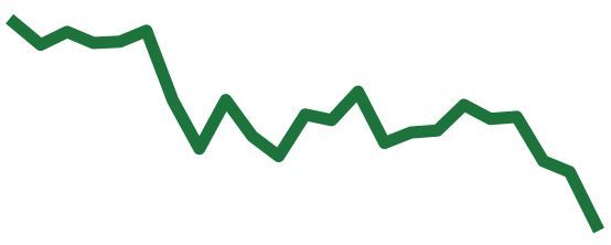
hard negative samples) and push apart their representations, L = Lpred + λLcl (8)4 Experiments 250
Ground truth
200
Traffic Flow
4.1 Experimental Setup GWN
150 GWN w/ STGCL
Datasets We evaluate the performance of STGCL on three 100
real-world traffic datasets: PEMS-BAY (Li et al. 2018), 50
PEMS-04 (Guo et al. 2019), and PEMS-08 (Guo et al. 2019). 02/24/2018 00:00-24:00
0
The datasets are collected by the Caltrans Performance Mea- 0 4 8 12 16 20 24
surement System (Chen et al. 2001). There are three kinds
of traffic measurements contained in the raw data, including Figure 5: Visualization of 60 minutes-ahead predictions on
traffic flow, average speed, and average occupancy. These a snapshot of the PEMS-04 test set.
traffic readings are aggregated into 5-minute windows, re-
sulting in 288 data points per day. We use the 12-step histor- 37 2 33
Contrastive GWN
ical data to predict the next 12 steps. Z-score normalization 33 Forecasting 3 30 GWN w/ STGCL
Contrastive Loss
Avg. Train MAE
Avg. Val. MAE
is applied to the input data. The adjacency matrix is con- 29 4 27
structed by road network distance with a thresholded Gaus-
25 5 24
sian kernel (Shuman et al. 2013). The datasets are divided
into three parts for training, validation, and test with a ratio 21 6 21
of 7:1:2 on PEMS-BAY, and 6:2:2 on PMES-04 and PEMS- 17
0 20 40 60 80 100
7 18
0 20 40 60 80 100
08. The dataset statistics are provided in Table 1. Epoch Epoch
Table 1: Dataset statistics. See more details in Appendix. Figure 6: The left part shows the training curve of forecast-
ing MAE and contrastive loss by using GWN w/ STGCL
Datasets #Nodes #Edges #Time steps on PEMS-04. The right part shows the validation MAE of
PEMS-BAY 325 2,369 52,116 GWN w/ STGCL against pure GWN on PEMS-04.
PEMS-04 307 340 16,992
PEMS-08 170 295 17,856
absolute percentage error (MAPE). More details about the
experimental settings can be found in Appendix.
Base Models We use four base models that belong to
the following two classes: CNN-based models (GWN, MT- 4.2 Performance Comparison
GNN) and RNN-based models (DCRNN, AGCRN).
Table 2 presents the test MAE results of the average val-
• GWN: Graph WaveNet combines adaptive adjacency ues over all predicted horizons and three specific horizons
matrix with graph convolution and uses dilated casual (15, 30, and 60 minutes). The complete table that include
convolution (Wu et al. 2019). MAE, RMSE, MAPE, and the specific settings for the re-
• MTGNN: A GNN framework designed for multivariate ported results are provided in Appendix. Our results show
time series forecasting. It proposes a graph learning mod- that STGCL achieves consistent improvements across all
ule and applies graph convolution with mix-hop propaga- base models on all datasets, which verifies the effectiveness
tion and dilated inception layer (Wu et al. 2020). of using contrastive loss and suggests that STGCL is model-
• DCRNN: Diffusion Convolution Recurrent Neural Net- agnostic, i.e., it can be applied to both CNN-based and
work, which integrates diffusion convolution into RNNs RNN-based model architectures. Note that particularly on
in an encoder-decoder manner (Li et al. 2018). the best performing models such as GWN and MTGNN, the
• AGCRN: This approach develops two adaptive modules improvements from STGCL are in many cases several times
to enhance graph convolution and combines them into the standard deviation, especially on PEMS-04 and PEMS-
RNNs (Bai et al. 2020). 08, suggesting that they are statistically significant. It is also
worth mentioning that some of the improvements derived
Implementation Details We use PyTorch to implement from STGCL are even larger than using an advanced model.
all the base models and our method. All the experiments in For instance, GWN obtains an average MAE of 19.33 on
this section are repeated 5 times with different seeds. We PEMS-04, while the MAE is reduced to 18.88 after apply-
basically employ the default settings of base models from ing STGCL, better than MTGNN (MAE=19.09). In addi-
their source code, such as model configurations, batch size, tion, the standard deviation of STGCL is generally smaller
optimizer, learning rate, and gradient clipping. The settings than that of the base model, which indicates that STGCL can
of STGCL follow the same as in base models’ implementa- provide additional stability.
tion, except that we don’t apply weight decay, as this will Another important observation in Table 2 is that STGCL
introduce another term in the loss function. The maximum achieves larger improvements for long-term predictions,
number of epochs in the experiments is fixed to 100. The e.g., at the 60-minute horizon with bold fonts. To investi-
temperature τ is set to 0.1 after tuning within the range of gate it, we use GWN as the base model and randomly select
{0.05, 0.1, 0.15, 0.2, 0.25}. We adopt three kinds of metrics a sensor (#200) from PEMS-04 for a case study. Figure 5 vi-
to evaluate the model performance, including mean absolute sualizes the 60 minutes-ahead prediction results against the
error (MAE), root mean squared error (RMSE), and mean ground truth on a snapshot of the test data. It can be seen thatTable 2: Test MAE results of the base models and our method on PEMS-BAY, PEMS-04, and PEMS-08. min: minutes.
PEMS-BAY PEMS-04 PEMS-08
Methods
Avg. 15 min 30 min 60 min Avg. 15 min 30 min 60 min Avg. 15 min 30 min 60 min
GWN 1.59±.01 1.31±.00 1.64±.01 1.97±.03 19.33±.11 18.20±.09 19.32±.13 21.10±.18 14.78±.03 13.80±.05 14.75±.04 16.39±.09
w/ STGCL 1.54±.00 1.29±.00 1.61±.00 1.88±.01 18.88±.04 17.93±.04 18.87±.04 20.40±.09 14.61±.03 13.67±.04 14.61±.03 16.09±.05
MTGNN 1.59±.01 1.34±.02 1.66±.01 1.94±.02 19.09±.04 18.32±.05 19.10±.05 20.39±.09 15.34±.09 14.36±.06 15.34±.10 16.91±.16
w/ STGCL 1.56±.01 1.32±.00 1.63±.01 1.89±.01 18.68±.04 17.99±.03 18.72±.05 19.88±.07 14.88±.04 14.04±.05 14.90±.05 16.23±.08
DCRNN 1.66±.05 1.34±.03 1.71±.05 2.09±.08 22.70±.21 19.99±.11 22.40±.19 27.15±.35 17.11±.25 15.23±.15 16.98±.25 20.27±.41
w/ STGCL 1.63±.00 1.32±.00 1.68±.00 2.05±.00 22.34±.13 19.82±.08 22.07±.12 26.51±.21 17.01±.20 15.19±.11 16.89±.19 20.09±.34
AGCRN 1.63±.01 1.37±.00 1.69±.01 1.99±.01 19.39±.03 18.53±.03 19.43±.06 20.72±.03 15.79±.06 14.58±.07 15.71±.07 17.82±.11
w/ STGCL 1.61±.01 1.35±.00 1.67±.01 1.96±.01 19.13±.05 18.31±.04 19.17±.06 20.39±.03 15.62±.07 14.51±.05 15.56±.06 17.51±.10
Table 3: Effects of λ on PEMS-04 and PEMS-08. Table 4: Effects of threshold rf on PEMS-04 and PEMS-08.
PEMS-04 PEMS-08 Filtering PEMS-04 PEMS-08
Lambda
GWN AGCRN GWN AGCRN threshold GWN AGCRN GWN AGCRN
0.01 18.91±0.14 19.33±0.09 14.71±0.02 15.82±0.06 0 min 19.00±0.07 19.26±0.04 14.67±0.03 15.73±0.06
0.05 18.91±0.06 19.30±0.11 14.61±0.03 15.67±0.04 30 min 18.93±0.03 19.13±0.05 14.63±0.02 15.70±0.13
0.1 18.91±0.06 19.19±0.04 14.64±0.06 15.62±0.07 60 min 18.88±0.04 19.16±0.04 14.61±0.03 15.62±0.07
0.5 18.88±0.04 19.16±0.04 14.69±0.06 15.76±0.05 90 min 18.93±0.07 19.28±0.03 14.65±0.04 15.76±0.08
1.0 18.95±0.11 19.29±0.11 14.72±0.05 15.89±0.06 120 min 18.94±0.09 19.34±0.11 14.68±0.07 15.75±0.10
GWN w/ STGCL outperforms the counterpart, especially at atively stable and do not have an obvious trend. The reason
the sudden change (see the red rectangle). A plausible ex- could be that masking a certain fraction of entries to zero dis-
planation to this is that STGCL has learned discriminative turbs input a lot, but the disturbance injected by other aug-
representations by receiving signals from contrastive task mentations is considered reasonable by the models. 4) Input
during training, hence it can successfully distinguish some masking with a 1% ratio achieves most of the best perfor-
distinct patterns (like sudden changes). mance across the applied models and datasets. We thereby
Besides, we plot the learning curves of the two losses suggest using this setting in other datasets for initiatives.
(Lpred and Lcl ) in Figure 6 (left-hand side) to further ver-
ify the learning of the dual tasks. The reason why the con- 4.4 Effects of Contrastive Loss
trastive loss is less than 0 is that the denominator of the con- We show the effects of loss term trade-off parameter λ in Ta-
trastive loss does not contain the numerator, thus their ratio ble 3 and the filtering threshold rf in Table 4. Input masking
can be greater than 1. While on the right-hand side of the with a 1% ratio is used as the default augmentation setting.
figure, we plot the trends of the validation MAE. It is clear The results show that tuning λ within {0.01, 0.05, 0.1, 0.5,
that STGCL achieves better performance and is more stable 1.0} is sufficient to find the best value and the PEMS-04
than the pure GWN model. Next, we select one CNN-based dataset prefers a larger λ than that on the PEMS-08 dataset.
model (GWN) and one RNN-based model (AGCRN) as rep- For the negative filtering operation, we show that the fil-
resentatives to show the effects of each component. tering threshold rf works best when set to 30 or 60 minutes,
which demonstrates the effectiveness of our simple solution.
4.3 Effects of Data Augmentation We also notice that when rf is set to 120 minutes, some re-
We show the effects of different augmentation methods by sults are worse than when rf is set to 0. The reason is that the
tuning the hyper-parameter related to that method in Fig- threshold of 120 minutes filters out too many negatives and
ure 7. We highlight the best performance achieved by each the contrastive task becomes too easy, hence the model may
model on each augmentation method in the figure. For in- not be able to learn useful discrimination knowledge. One
put smoothing, the fixed entries Eis is set to 20 after tuning insight we can draw from the experimental results is that by
within the range of {16, 18, 20, 22}. filtering out the hardest negative samples (the most semanti-
From the figures, we have the following observations: 1) cally similar samples), we can help the contrastive loss focus
all the proposed data augmentations can successfully im- on the true negative samples. On the other hand, filtering too
prove performance over the base models. 2) The best per- many negatives makes the contrastive task meaningless and
formance achieved by each augmentation method has little leads to performance degradation.
difference, though the semantics of each method is different Our negative filtering operation is also more efficient in
(e.g., temporal shifting and input smoothing are performed measuring the similarity of two time series sequences than
in the time and frequency domain, respectively). This indi- existing methods such as dynamic time warping (Berndt and
cates that STGCL is not sensitive to augmentation seman- Clifford 1994) or Pearson correlation coefficient. The reason
tics. 3) Input masking is significantly affected by the distur- is that our method only needs to compare the starting time
bance magnitude, while other augmentation methods are rel- of each sample and does not involve other computations.19.30 19.30 19.30 19.30
AGCRN 19.19
GWN
Avg. Test MAE
19.20 19.20 19.20 19.20
19.13 19.18
19.10 19.10 19.10 19.10 19.10
19.00 19.00 19.00 19.00
18.92 18.91 18.89
18.90 18.90 18.88 18.90 18.90
10% 15% 20% 25% 30% 1% 5% 10% 15% 20% 0.10 0.30 0.50 0.70 0.90 0.10 0.30 0.50 0.70 0.90
Edge masking ratio rem Input masking ratio rim Temporal shifting range rts Input smoothing range ris
(a) PEMS-04
15.80 15.80 15.80 15.80
15.66
Avg. Test MAE
15.70 AGCRN 15.70 15.70 15.70
GWN 15.62 15.68
15.60 15.60 15.60 15.60 15.66
14.70 15.00 14.70 14.66 14.70
14.61 14.63
14.61
14.60 14.60 14.60 14.60
10% 15% 20% 25% 30% 1% 5% 10% 15% 20% 0.10 0.30 0.50 0.70 0.90 0.10 0.30 0.50 0.70 0.90
Edge masking ratio rem Input masking ratio rim Temporal shifting range rts Input smoothing range ris
(b) PEMS-08
Figure 7: Effects of different augmentation methods on the PEMS-04 and PEMS-08 datasets.
5 Related Work multi-view contrasting by using a diffused graph as a global
5.1 Deep Learning for Spatio-Temporal Graphs view of the original graph, after which the MI is maximized
in a cross-view and cross-scale manner.
STG forecasting is a typical problem in smart city efforts, For same-scale contrasting, graph elements are contrast-
facilitating a wide range of applications, such as traffic fore- ing in an equal scale, such as node-node and graph-graph
casting and air quality prediction. Recently, spatio-temporal contrasting. Regarding the definition of positive/negative
graph neural networks have become the dominant class for pairs, the approaches can be further divided into context-
modeling STG. They either integrate graph convolutions based and augmentation-based. The context-based methods
with CNNs or RNNs to capture the spatial and temporal generally utilize random walks to obtain positive samples.
dependencies within STG. As a pioneering work, DCRNN Our work lies in the scope of augmentation-based meth-
(Li et al. 2018) considers traffic flow as a diffusion process ods, where the positive samples are generated by disturbance
and proposes a novel diffusion convolution to capture spa- on nodes or edges. A representative work GraphCL (You
tial dependencies. To improve training speed, GWN (Wu et al. 2020) adopts four graph augmentations to form posi-
et al. 2019) adopts a complete convolutional structure, which tive pairs and contrasts at graph level. GCA (Zhu et al. 2021)
combines graph convolution with dilated casual convolution works at the node level and performs augmentations that are
operation. It also proposes an adaptive adjacency matrix as adaptive to the graph structure and attributes.
a complement to the predefined one. In addition, GeoMAN
(Liang et al. 2018) and ASTGCN (Guo et al. 2019) intro-
duce attention mechanisms on both spatial and temporal di- 6 Conclusion and Future Work
mensions to capture the dynamics of spatio-temporal cor- This study explores the potential of utilizing contrastive
relations. The recent developments in this field show the learning techniques to improve STG forecasting perfor-
following trends: make the adjacency matrix fully learnable mance. In particular, we have presented STGCL, a novel
(Bai et al. 2020), and developing modules to jointly capture and model-agnostic framework that enhances the forecast-
spatial and temporal dependencies (Song et al. 2020). ing task with a supplementary contrastive task. Four STG-
specific augmentations that differ from the methods on the
5.2 Contrastive Learning on Graphs general graphs are devised to construct positive pairs. We
Recently, contrastive representation learning approaches on also propose a rule-based strategy to alleviate an inherent
graphs have attracted significant attention. According to the shortcoming of the unsupervised contrastive method, i.e., ig-
taxonomy from a recent survey (Liu et al. 2021), exist- noring the sample’s semantic similarity. The extensive ex-
ing methods can be divided into cross-scale contrasting and periments on four state-of-the-art models and three real-
same-scale contrasting. world datasets have demonstrated the superiority of STGCL.
Cross-scale contrasting refers to the scenario that the con- Besides, we have noticed that each component of STGCL
trastive elements are in different scales. For example, a rep- still has space to improve. In the future, we plan to leverage
resentative work named DGI (Velickovic et al. 2019) con- adaptive data augmentation techniques to identify the im-
trasts between the node and graph-level representations via portance of edges/nodes, thus treating them differently when
mutual information (MI) maximization, thus gaining bene- generating augmented views. Another direction is designing
fits from flowing global information to local representations. a learnable negative filtering method that can dynamically
MVGRL (Hassani and Khasahmadi 2020) further suggests a assign weights to hard negatives, rather in a rule-based way.References Shuman, D. I.; Narang, S. K.; Frossard, P.; Ortega, A.; and
Bai, L.; Yao, L.; Li, C.; Wang, X.; and Wang, C. 2020. Vandergheynst, P. 2013. The emerging field of signal pro-
Adaptive Graph Convolutional Recurrent Network for Traf- cessing on graphs: Extending high-dimensional data analy-
fic Forecasting. In Proceedings of Advances in Neural In- sis to networks and other irregular domains. IEEE signal
formation Processing Systems, volume 33, 17804–17815. processing magazine, 30: 83–98.
Berndt, D. J.; and Clifford, J. 1994. Using dynamic time Song, C.; Lin, Y.; Guo, S.; and Wan, H. 2020. Spatial-
warping to find patterns in time series. In KDD workshop, temporal synchronous graph convolutional networks: A new
volume 10, 359–370. framework for spatial-temporal network data forecasting. In
Proceedings of the AAAI Conference on Artificial Intelli-
Chen, C.; Petty, K.; Skabardonis, A.; Varaiya, P.; and Jia, Z. gence, volume 34, 914–921.
2001. Freeway performance measurement system: mining
Veličković, P.; Cucurull, G.; Casanova, A.; Romero, A.; Lio,
loop detector data. Transportation Research Record, 1748:
P.; and Bengio, Y. 2018. Graph attention networks. In Pro-
96–102.
ceedings of International Conference on Learning Repre-
Chen, T.; Kornblith, S.; Norouzi, M.; and Hinton, G. 2020. sentations.
A simple framework for contrastive learning of visual rep- Velickovic, P.; Fedus, W.; Hamilton, W. L.; Liò, P.; Ben-
resentations. In Proceedings of International conference on gio, Y.; and Hjelm, R. D. 2019. Deep Graph Infomax. In
machine learning, 1597–1607. Proceedings of International Conference on Learning Rep-
Guo, S.; Lin, Y.; Feng, N.; Song, C.; and Wan, H. 2019. At- resentations.
tention based spatial-temporal graph convolutional networks Wu, Z.; Pan, S.; Long, G.; Jiang, J.; Chang, X.; and Zhang,
for traffic flow forecasting. In Proceedings of the AAAI Con- C. 2020. Connecting the dots: Multivariate time series fore-
ference on Artificial Intelligence, volume 33, 922–929. casting with graph neural networks. In Proceedings of the
Hassani, K.; and Khasahmadi, A. H. 2020. Contrastive 26th ACM SIGKDD International Conference on Knowl-
multi-view representation learning on graphs. In Proceed- edge Discovery & Data Mining, 753–763.
ings of International Conference on Machine Learning, Wu, Z.; Pan, S.; Long, G.; Jiang, J.; and Zhang, C. 2019.
4116–4126. Graph wavenet for deep spatial-temporal graph modeling. In
Hu, Z.; Dong, Y.; Wang, K.; Chang, K.-W.; and Sun, Y. Proceedings of International Joint Conference on Artificial
2020. Gpt-gnn: Generative pre-training of graph neural net- Intelligence.
works. In Proceedings of the 26th ACM SIGKDD Interna- Yi, X.; Zheng, Y.; Zhang, J.; and Li, T. 2016. ST-MVL:
tional Conference on Knowledge Discovery & Data Mining, filling missing values in geo-sensory time series data. In
1857–1867. Proceedings of International Joint Conference on Artificial
Kipf, T. N.; and Welling, M. 2017. Semi-supervised classi- Intelligence.
fication with graph convolutional networks. In Proceedings You, Y.; Chen, T.; Sui, Y.; Chen, T.; Wang, Z.; and Shen, Y.
of International Conference on Learning Representations. 2020. Graph contrastive learning with augmentations. In
Li, M.; and Zhu, Z. 2021. Spatial-Temporal Fusion Graph Proceedings of Advances in Neural Information Processing
Neural Networks for Traffic Flow Forecasting. In Pro- Systems, volume 33.
ceedings of the AAAI Conference on Artificial Intelligence, Yu, F.; and Koltun, V. 2016. Multi-scale context aggrega-
4189–4196. tion by dilated convolutions. In Proceedings of International
Li, Y.; Yu, R.; Shahabi, C.; and Liu, Y. 2018. Diffusion Conference on Learning Representations.
convolutional recurrent neural network: Data-driven traffic Zeng, J.; and Xie, P. 2021. Contrastive self-supervised learn-
forecasting. In Proceedings of International Conference on ing for graph classification. In Proceedings of the AAAI Con-
Learning Representations. ference on Artificial Intelligence.
Liang, Y.; Ke, S.; Zhang, J.; Yi, X.; and Zheng, Y. 2018. Ge- Zhang, H.; Cisse, M.; Dauphin, Y. N.; and Lopez-Paz, D.
oman: Multi-level attention networks for geo-sensory time 2017. mixup: Beyond empirical risk minimization. In Pro-
series prediction. In Proceedings of International Joint Con- ceedings of International Conference on Learning Repre-
ference on Artificial Intelligence, volume 2018, 3428–3434. sentations.
Liu, Y.; Pan, S.; Jin, M.; Zhou, C.; Xia, F.; and Yu, P. S. 2021. Zhang, J.; Zheng, Y.; and Qi, D. 2017. Deep spatio-temporal
Graph self-supervised learning: A survey. arXiv preprint residual networks for citywide crowd flows prediction. In
arXiv:2103.00111. Proceedings of the AAAI Conference on Artificial Intelli-
Oord, A. v. d.; Li, Y.; and Vinyals, O. 2018. Representation gence.
learning with contrastive predictive coding. arXiv preprint Zhu, Y.; Xu, Y.; Yu, F.; Liu, Q.; Wu, S.; and Wang, L. 2021.
arXiv:1807.03748. Graph contrastive learning with adaptive augmentation. In
Proceedings of the Web Conference 2021, 2069–2080.
Pan, Z.; Liang, Y.; Wang, W.; Yu, Y.; Zheng, Y.; and Zhang,
J. 2019. Urban traffic prediction from spatio-temporal data
using deep meta learning. In Proceedings of the 25th ACM
SIGKDD International Conference on Knowledge Discov-
ery & Data Mining, 1720–1730.You can also read