Synthetic Portnet Generation with Controllable Complexity for Testing and Benchmarking - Benny Akesson
←
→
Page content transcription
If your browser does not render page correctly, please read the page content below
Synthetic Portnet Generation with
    Controllable Complexity for Testing and
                 Benchmarking

    Madiou Diallo1,2 , Benny Akesson1,2 , Debjyoti Bera1 , and Ronald Begeer1
                       1
                          ESI (TNO), Eindhoven, the Netherlands
               2
                   University of Amsterdam, Amsterdam, the Netherlands

        Abstract. There are many classes of Petri nets for describing commu-
        nicating systems. Some of these guarantee important properties, such as
        termination in the case of portnets. There are also many methods and
        tools available for their analysis and synthesis. However, when devel-
        oping new methods, or benchmarking against existing ones, it is often
        helpful to quickly generate large sets of random models satisfying certain
        properties and user-defined rules.
        This paper presents a heuristic-driven method for synthetic generation of
        random portnets based on refinement rules. The method considers three
        user-specified complexity parameters: the expected number input and
        output places, and the prevalence of non-determinism in the skeleton
        of the generated net. An implementation of this method is available
        as an open-source Python tool. Experiments demonstrate the relations
        between the three complexity parameters and investigate the boundaries
        of the proposed method.

1     Introduction
The theory of communicating systems have been extensively studied over the
past few decades [8, 16]. A lot of the results on their modeling and analysis are
being increasingly applied in context of component-based software development
in industry, such as in the development of medical devices [10], radars [1], and
lithography machines [18]. Such systems usually consist of many asynchronously
communicating components that cooperate to realize a set of functionality. It is
essential for safe and reliable operation that such systems are designed correctly
and that the interactions between components, specified by their interfaces, are
guaranteed to be free from problems, such as deadlocks, livelocks, or buffer over-
flows.
    Petri nets [14] are a popular formalism for modeling and analysis of asyn-
chronous communicating systems. In the context of service-oriented architectures
    Copyright c 2021 for this paper by its authors. Use permitted under Creative Com-
    mons License Attribution 4.0 International (CC BY 4.0).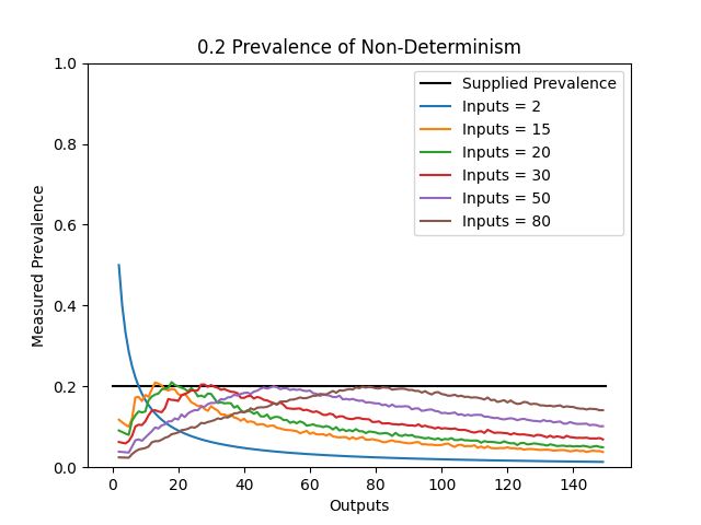
and distributed control systems, there exist a lot of work [16] around architec-
tural frameworks, interaction patterns, and classes of Petri nets guaranteeing
some sort of termination property [2, 3]. Next to that, there are also a lot of
methods and tools available for their analysis (structural or behavioral) and syn-
thesis, e.g. adapter generation [7,12,16]. Development of new methods and tools,
as well as benchmarking of existing ones, benefit from the ability to synthetically
generate large sets of random input models satisfying certain properties and con-
straints [17], e.g. the size and complexity of the generated net. Such synthetically
generated models reduce or even eliminate the time-consuming process of man-
ually creating large sets of input models to identify bugs or for benchmarking
against existing methods and their implementations.
     The need for synthetic generation of models with controllable characteristics
is recognized in the modelling community, and tools already exists for generating
task graphs [6], synchronous data-flow graphs [15], as well as Petri nets [17]. Sim-
ple place transition nets are not suitable for modeling component-based systems.
The class of open nets [9] is more appropriate, as it explicitly models communica-
tion aspects. Components communicate with each other over interfaces modeled
as portnets [3], which are a class of open nets with various structural constraints,
guaranteeing the freedom of deadlocks, livelocks and unbounded behaviour, even
in the presence of multiple clients. However, there is currently no method to
synthetically generate random portnets with controllable parameters, limiting
efficient development and benchmarking of methods and tools applicable to this
class of nets, e.g. [7, 11, 12] and the software interfaces they model [1, 10].
     This paper addresses this problem through four main contributions:

 1. Three complexity metrics for portnets are defined, the number of input and
    output places in net, as well as the prevalence of non-determinism within its
    skeleton (i.e. the net obtained after discarding the input and output places),
    and we discuss their inherent relation for nets generated from refinement
    rules.
 2. A heuristic method based on refinement rules for quick synthetic generation
    of random portnets that considers the three complexity metrics as input
    parameters is proposed.
 3. An implementation of the proposed method in an open-source Python tool.
 4. An experimental demonstration of the relations between the complexity pa-
    rameters, and an evaluation of how well the proposed method and tool satisfy
    them.

    The rest of this paper is organized as follows. Section 2 presents the necessary
preliminaries. Section 3 then introduces the three complexity parameters and
discuss their inherent relation, before Section 4 introduces the proposed method
for synthetic port net generation. Section 5 discusses the implementation of the
proposed method in a tool, which is then experimentally evaluated in Section 6.
Section 7 concludes the paper.
2     Preliminaries

This section introduces the preliminaries that our proposed method for synthetic
generation of random portnets builds on. Section 2.1 introduces relevant Petri
Net concepts after which Section 2.2 presents a set of refinement rules.

2.1   Petri Nets

A Petri net is a tuple N = (P, T, F ), where P is the set of places; T is the set of
transitions such that P ∩T = ∅ and F is the flow relation F ⊆ (P ×T )∪(T ×P ).
We refer to elements from P ∪ T as nodes and elements from F as arcs. We
define the preset of a node n as • n = {m|(m, n) ∈ F } and the postset as
m• = {n|(m, n) ∈ F }. A path ν in a Petri net N of length n ∈ N is a function
ν : 1, . . . , n → (P ∪ T ) such that (ν(i), ν(i + 1)) ∈ F for all 1 ≤ i < n. We denote
a path of length n by ν = hx1 , . . . , xni i, where xi = ν(i) for all q ≤ i ≤ n.
    A Petri net is a state machine (S-Net) if and only if the preset and postset
of all of its transitions are never greater than one. In a state machine, a place is
called a split if its postset is greater than one. Likewise, it is a join if its preset
is greater than one. A Petri net is a workflow net (WFN) if there exists exactly
one place with an empty preset, called the initial place, exactly one place with
an empty postset, called the final place, and all nodes are on a path from the
initial to the final place. A workflow net (WFN) that is also an S-Net is called
a state machine workflow net (S-WFN).
    An open Petri net (OPN) is an extension of classical Petri nets, ideal for
modeling asynchronous communicating systems. OPNs have a distinguished set
of interface places partitioned into a subset of input places, I, and output places,
O, representing the interfaces of the net. All places (including inputs and out-
puts) and transitions are pairwise disjoint. The net obtained by discarding the
interface places and their associated arcs of an OPN is called its skeleton. The
skeleton of an OPN defines its internal behavior. If the skeleton of an OPN is a
WFN then the OPN is called an open workflow net (OWN). If the skeleton of
an OPN is an S-WFN then the OPN is called a state machine open workflow net
(S-OWN). Two OPNs can be composed by fusing their shared interface places.
We say two OPNs are composable if and only if the set of input places of one
net is equal to the set of output places of the other net, and vice versa. Two
examples of server and client S-OWNs that have been composed are shown in
Figure 1. The interface places are visually distinguished by putting them inside a
black rectangle. Tokens in these places represent messages being communicated
between the server and the client.
    A portnet is an S-OWN with four constraints on the relation between tran-
sitions and interface places and the paths through it.

 1. A transition is connected to exactly one input place or output place. As a
    consequence, a transition is either representing a send or a receive operation.
 2. Each interface place is connected to exactly one transition.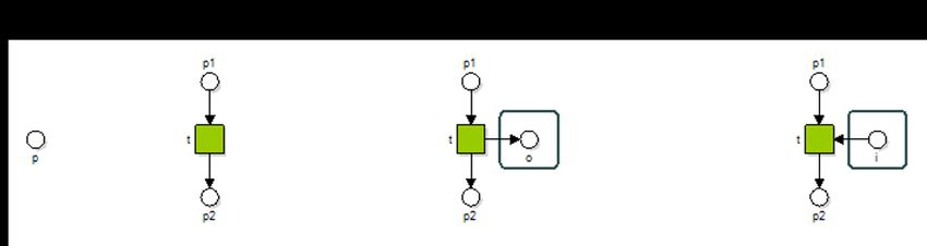
(a) Choice property violation (b) Leg property violation
Fig. 1: Two examples of server and client open nets that have been composed to
form closed nets. These nets are not portnets because of property violations.
3. A portnet must satisfy the choice property, which requires all transitions
belonging to the postset of a place to communicate in the same direction,
i.e. they must all either send or receive.
4. A portnet must satisfy the leg property. A path in a portnet is called a leg
if it is a path from a split to a join. The initial place is considered as a split
and the final place as a join. The leg property requires every leg in a portnet
to have at least one send transition and one receive transition.
The two servers (and clients) in Figure 1 are S-OWN, but not portnets. While
they both satisfy the first two constraints, the initial place in Figure 1a violates
the choice property. This causes a deadlock with tokens in interface places q1
and q2 if the server and client follow different paths. In contrast, the net in
Figure 1b satisfies the choice property, but the path hp1, t3, p2, t4, p1i violates
the leg property since it only has communication in one direction. This allows
the server to execute this path without synchronizing with the client, possibly
resulting in an unbounded number of tokens in interface places q2 and q3.
For a formal definition of all these concepts, please refer to [3]. The four
portnet constraints guarantee the weak termination property, which promises
freedom of deadlocks, livelocks and unbounded behavior. A portnet is called a
client (server) portnet if all transitions in the postset of the initial place are of
type send (receive). A server portnet can be composed with one or more client
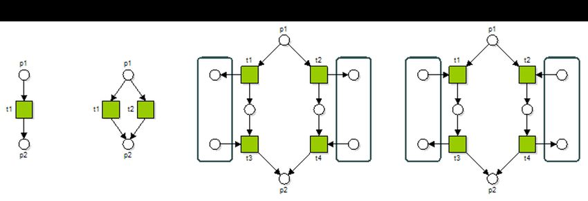
portnets if and only if they are composable and their skeletons are isomorphic.2.2 Refinement Rules The work in [3] presents refinement rules to construct portnets starting from a single place. The four refinement rules guarantee that the resulting net is always a portnet. For each of the four refinement rules, we distinguish two categories: base rules and modified rules. Base rules form the starting point for refinement. They are applied to a transition or place and generate a new structure within the portnet. In conjunction with a modified rule, the structure is altered in a way such that it adheres to the four portnet constraints. Specifically, the modified rules determine the direction of communication and ensure the leg and choice properties are satisfied. In the remainder of this paper, we denote a base rule as Rx and the corresponding modified rules as Rx0 /Rx”. We continue by briefly describing each of the four refinement rules. A graphical representation of each rule can be seen in Figure 2. R0: Default Place Refinement The default rule, R0, forms the base of the refinement rules. It refines a place p by expanding it into two new places, p1 and p2 connected by a transition, t. The modified rules R00 and R000 connect the added transition to an input place, i, or output place, o, to ensure that the portnet constraints are satisfied. Rule R0 is visualized in Figure 2a. R1: Transition Refinement Rule R1 is similar to R0, but refines a transition rather than a place. It refines a transition t by expanding it into t1 and t2 and connecting them through a place, p. The modified rules connect each transition to an input place, i, or an output place, o, to satisfy the structural constraints. Note that both transitions cannot connect to input places or output places, since this would violate the leg property. This rule is shown in Figure 2b. R2: Non-deterministic Transition Refinement The non-deterministic tran- sition refinement rule R2 expands a transition, t1 by duplicating it. The newly created transition t2 has the same preset and postset, p1 and p2, as shown in Figure 2c. Like with the previous rules, the modified rules ensure that the four portnet constraints are satisfied. This means ensuring that t1 and t2 communi- cate in the same direction to satisfy the choice property and that each of the two legs contains communication in both directions to satisfy the leg property. R3: Cyclic Place Refinement When refining a place, p, R3 introduces a cyclic structure with a transition, t, as shown in Figure 2d. Note that the base rule of R3 violates the leg property. Consequently, the modified rules further expand the resulting structures and satisfy the leg property by ensuring communication in both directions. Note that R3 introduces a split in the net when applied to a place that already has an outgoing arc. This is always the case in this paper, since the only place without an outgoing arc in a workflow net is the final place, and applying this rule to that place violates its definition.
(a) Default Place Refinement

                           (b) Transition Refinement

                   (c) Non-deterministic Transition Refinement

                          (d) Cyclic Place Refinement

Fig. 2: The four refinement rules from [3], each with two modified versions that
ensure portnet constraints are satisfied.
3 Complexity Parameters
This section introduces the three user-specified complexity parameters and dis-
cusses their inherent relation in portnets generated using the refinement rules.
Note that this relation is independent from our proposed generation method.
3.1 Definition of Complexity Parameters
First, we introduce a measure of non-determinism present in a portnet. Given
a portnet N = (P, I, O, T, F ), we define prevalence of non-determinism, or just
prevalence for short, as
| {(p, t) ∈ F | p ∈ P ∧ | p• |> 1} |
ρ(N ) = (1)
| {(p, t) ∈ F | p ∈ P } |
We will refer to the set of arcs defined in the numerator as non-deterministic
arcs, i.e., the set of all outgoing arcs from split places of the net. The remaining
set of outgoing arcs from places that are not included in this set are referred to
as deterministic arcs.
This work considers three complexity parameters, (Iexp , Oexp , P rexp ) as input,
where Iexp > 0 is the expected number of input places, Oexp > 0, is the expected
number of output places, and, P rexp ∈ [0.0, 1.0] is the expected prevalence of
non-determinism in the generated net. The number of input places and the
number of output places are simple and intuitive complexity parameters for open
nets. Prevalence captures the complexity of the control flow and can be used as
an alternative to cyclomatic complexity [13] or the more elaborate Control-Flow
Complexity (CFC) metric [5].
By the definition of a portnet (see Section 2.1), there must be at least one
input place and one output place to satisfy the leg property. Furthermore, each
transition in a portnet is connected to exactly one input or output place and
vice versa. The parameters Iexp and Oexp hence directly determine the number
of transitions in the synthesized net.
Figure 3 shows an example portnet with four input places and four output
places. Observe the three split places initial, p2, and p3. The sum of outgoing arcs
from these places is six. Since the total number of arcs from places to transitions
is eight, the prevalence in the net is 86 = 0.75.
3.2 Influence of Refinement Rules on Complexity
We proceed by discussing the relation between the defined complexity parame-
ters in portnets generated using refinement rules. Note that all refinement rules
add nodes and arcs to the net being refined. Table 1 summarizes the number of
nodes and arcs added by each rule.
From the table, we make three observations. First, R0 is the only rule that
can add a single interface place (i.e., either an input place or an output place).
All other rules add an equal number of input and output places. Consequently,Fig. 3: Example portnet with characteristics (Iexp = 4, Oexp = 4, P rexp = 0.75)
Table 1: Elements added to the generated portnet through the application of
each refinement rule.
Deterministic Non-Deterministic
Rule Inputs Outputs Transitions Places
Arcs Arcs
R0 0/1a 1/0 1 1 1 0
R1 1 1 1 1 1 0
R2 2 2 3 2 1 2
R3 1 1 2 1 1/0b 1/2
a
For R00 / R000 , respectively
b
When applied to non-deterministic (split) / deterministic places, respectively
one or more applications of a modified rule of R0 must be applied when the
number of expected input places and output places are different. We also see
in Table 1 that this rule only adds a deterministic arc. Unless the current net
(under construction) is already fully deterministic, P rcur = 0, it follows from
Equation (1) that the overall prevalence of non-determinism of the generated net
is reduced when the rule is applied. An implication of this is that the prevalence
of non-determinism is generally lower in random nets where the number of input
places and output places are not equal. We later demonstrate this experimentally
in Section 6.
Secondly, we note that only rules R2 and R3 introduce non-determinism, as
they introduce a split from the original path. For this reason, we refer to these
rules as the set of non-deterministic rules, while R0 and R1 comprise the set of
deterministic rules.
Thirdly, as previously mentioned in Section 2.2, a place is always a split place
after rule R3 has been applied to it. Figure 3 illustrates this. In this net, R3 has
just been applied on p2 and p3. Consequently, as there are then two outgoingarcs from both of those places they both become split places. Each application of
R3 has hence added one deterministic arc and two non-deterministic arcs, one of
which was previously deterministic. In total, the number of deterministic arcs is
hence unchanged, while the number of non-deterministic arcs increased by two.
When R3 is applied to a place that is already non-deterministic (split), e.g. to
p2 again, one deterministic and one non-deterministic arc is added. It follows
from Table 1 and Equation (1) that the prevalence of non-determinism in a net
is maximally increased when applying rule R3 to deterministic place.
4 Portnet Generation Method
This section presents our proposed heuristic method for generation of random
portnets. First, we discuss the order in which the refinement rules can be applied
in Section 4.1, before presenting our algorithm for selecting and applying them
to satisfy the user-specified complexity parameters in Section 4.2.
4.1 Allowed Ruleset
After introducing the refinement rules, the complexity parameters and their rela-
tions, we proceed by presenting the allowed ruleset. This ruleset determines how
the refinement rules from Section 2.2 can be applied in sequence on structures
within the portnet, starting from a single place. The output of one rule becomes
the input for the next. The applied ruleset hence ensures basic compatibility
between the rules, i.e. that a transition refinement cannot be applied to a net
comprising only a single place.
Figure 4 illustrates the allowed ruleset. Nodes in the figure represent appli-
cations of rules and the edges determine the rules that may subsequently be
applied. Any sequence of rules, starting from a single place pstart and ending at
any modified rule Rx0 is referred to as a refinement iteration. As seen in Fig-
ure 4, the single place pstart that serves as a starting point for the iteration can
be refined using either R0 or R3, since these are the only rules applicable to a
single place. This process then continues on the resultant of the refinement until
a modified rule causes termination. The resulting structure is the output of one
refinement iteration. As can be observed from the state machine, all refinement
iterations consist of one or more base-rules. However, each refinement iteration
comprises only one modified rule after which the iteration is complete.
4.2 Generation Algorithm
We now present our portnet generation algorithm. Given the three user-specified
complexity parameters as input, the algorithm generates a random portnet that
attempts to adhere to these parameters. The pseudo code of the algorithm is
shown in Algorithm 1. We continue by discussing this algorithm in more detail.
The algorithm starts from a portnet N comprising a single initial place
(Line 1). It then initializes three variables Icur , Ocur , and P rcur , which rep-
resent the remaining number of input places and output places to add to theR10
R00 R1
R0
R0” R1”
pstart
R3 R30 R2 R20
R3” R2”
Fig. 4: Valid sequences of rules within a refinement iteration.
portnet N , as well as its current prevalence (Line 2). For convenience, we encode
the set of deterministic and non-deterministic rules, respectively, as refinement
iterations. The refinement iterations in the set of deterministic rules contain all
sequences of refinement rules in the allowed ruleset that start from a single place
and terminate with the modified rules of R0 and R1, respectively (Line 3). Con-
versely, the refinement iterations in the set of non-deterministic rules contain
the sequences that terminate with the modified rules of R2 and R3, respectively
(Line 5).
While there are still more input or output places to add to the current net
(Line 8), new refinement iterations are selected and applied. Selection of a refine-
ment iteration starts by first computing the prevalence of the current portnet,
P rcur , using Equation (1) (Line 9). If the current prevalence is less than the
expected value provided by the user, the set of non-deterministic refinement it-
erations is used to increase it. However, this is only possible if there is at least
one input place and one output place left to add to ensure that at least one rule
(R3) in the set can be applied without exceeding the expected number of inputs
and outputs (Line 10). Otherwise, if the current prevalence is greater than or
equal to the expected value, or if there is not enough remaining inputs and out-
puts, the set of deterministic iterations is used instead (Line 11). This contains
rule R0, which can be applied for any number of remaining input and output
places. This simple mechanism steers the prevalence towards the expected value,
while being mindful of the expected number of inputs and outputs.
Once the appropriate set of refinement iterations has been chosen, a refine-
ment iteration is selected from the set along with a place to which it should
be applied (Line 12). This selection is random, but subject to the constraintthat a refinement iteration that contains R3 cannot be selected together with
the initial or final place. This is because such a refinement would violate the
definitions of those places, as an initial place must have an empty preset and
a final place an empty postset. The selected refinement iteration may also not
exceed the remaining number of input and output places. The number of added
input and output places is inferred by looking at the last rule in the sequence,
which is always a modified rule, for which the number of added input and output
places are shown in Table 1. Next, we subtract the number of input and output
places that the selected refinement iteration adds to the generated net (Lines 13
and 14).
Lastly, the refinement rules in the selected refinement iteration is applied, one
at a time (Lines 15-21). In case the refinement iteration contains a modified R3
rule that causes a choice property violation, the other modified rule is selected
instead to resolve the violation.
Algorithm 1 Synthetic Portnet Generation
Inputs: Expected number of inputs Iexp , outputs Oexp , and prevalence P rexp
Output: Portnet N approximating the inputs.
1: Let portnet N with exactly one place and this is the initial place.
2: Let Icur ← Iexp , Ocur ← Iexp , P rcur ← 0
3: Let detrules = {hR0, R00 i, hR0, R0”i, hR0, R1, R10 i, hR0, R1, R1”i}
4: . set of sequences of deterministic refinement rules
5: Let nondetRules = {hR0, R2, R20 i, hR0, R2, R2”i, hR3, R30 i, hR3, R3”i}
6: . set of sequences of non-deterministic refinement rules
7: Let ruleset be an empty sequence of refinement rules
8: while Icur and Ocur are not equal to zero do
9: P rcur ← ρ(N )
10: if P rcur < P rexp and Icur ≥ 1 and Ocur ≥ 1 then ruleset ← nondetrules
11: else ruleset ← detrules
12: Pick r ∈ ruleset and p ∈ PN , such that (p is not initial or final and r(0) 6= R3)
and (Icur and Ocur are greater than or equal to the inputs and outputs added to
the net introduced by r)
13: Subtract the number of inputs introduced by rule r from Icur
14: Subtract the number of outputs introduced by rule r from Ocur
15: while r is not empty sequence do
16: if r(0) = R30 or r(0) = R300 then
17: if refining place p with R30 causes a choice property violation then
18: r(0) ← R300
19: else r(0) ← R30
20: Refine place p of portnet N with rule r(0).
21: Remove rule r(0)5 Tool Implementation
The proposed method has been implemented in an open-source Python tool. The
source code of the project can be found on GitHub3 . The prototype tool was
built with modularity in mind and is therefore easily extendable. The addition
of new refinement rules or adding weights to the probabilities of rule selection is
hence straight-forward.
The tool is invoked on the command line along with the expected complexity
parameters, as shown in Figure 5. The basic format for invoking the tool is shown
below. For reproducibility, it is also possible to provide a seed for the random
number generator. If this is not provided, it is chosen at random.
python3 (inputs) (outputs) (prevalence of non-determinism)
The generated portnet is output in PNML4 format [4]. Since this work was
done in the context of software interfaces in cyber-physical systems [1], it is also
possible to generate a ComMA5 interface specification [10] with the same struc-
ture as the generated portnet. A manually made visualization of the generated
net is shown in Figure 6a. To give an intuitive feeling for the prevalence pa-
rameter, a second example with the same number of expected input and output
places, but a higher expected prevalence of non-determinism is shown in Fig-
ure 6b. Both generated nets contain the expected number of inputs and outputs.
The actual prevalence, P r, is closely approximated for the former net, while it
is exact for the latter.
Fig. 5: Command Line Portnet Generation (Iexp = 5, Oexp = 5, P rexp = 0.3)
3
github.com/Diallo/Synthetic-Interface-Generator
4
http://www.pnml.org/
5
https://esi.nl/research/output/tools/comma(a) Generated port- (b) Generated portnet with (Iexp = net with parameters 4, Oexp = 4, P rexp = 0.5|P r = 0.5) (Iexp = 4, Oexp = 4, P rexp = 0.3|P r = 0.25)
6   Experiments

This section experimentally demonstrates the inherent relation between the user-
specified complexity parameters, and evaluates the extent to which the proposed
method manages to satisfy them.
    For this experiment, portnets were generated by the tool for different combi-
nations of user-specified complexity parameters. The required number of input
and output places were taken from the set {2, 15, 20, 30, 50, 80} and the expected
prevalence of non-determinism from the set {0.2, 0.4, 0.6, 0.8}. In total, 40 port-
nets were generated for each combination of these parameters. The results of
the experiments are shown in Figure 7, where each subfigure corresponds to a
different value of expected prevalence of non-determinism. The six curves within
each subfigure denote the number of input places. Each subfigure hence shows
the average prevalence of non-determinism of the generated nets as a function
of the required number of output places, the other two parameters are fixed.

             (a) P rexp = 0.2                         (b) P rexp = 0.4

             (c) P rexp = 0.6                         (d) P rexp = 0.8

Fig. 7: Average observed prevalence of non-determinism as a function of the user-
specified complexity parameters for 40 generated portnets.
Four remarks can be made about the results. Firstly, we have verified that
the generated net always contains the expected number of input and output
places.
Secondly, in all subfigures, we see that when fixing the number of input
and output places to two, the generator tries to satisfy the expected prevalence
of non-determinism by selecting a non-deterministic rule. The generator tries
to match the parameter and creates a refinement iteration concluding with a
modified rule R2. The only alternative non-deterministic rule is R3, which may
not be applied to the initial or final place, as it would violate their definitions. The
application of rule R2 provides all required input and output places, immediately
causing the generation to stop no matter what the expected prevalence of non-
determinism was. The generated net has a prevalence of non-determinism of
P r= 0.5.
Thirdly, we see in Figures 7a and 7b that the expected prevalence of non-
determinism is closely approximated when the number of input and output places
are equal. This is the essence of what the proposed generation method is trying
to achieve. We also see that the prevalence of non-determinism monotonically re-
duces as the absolute difference between the number of input places and output
places increases. This experimentally demonstrates the inherent relation between
the complexity parameters when randomly using the refinement rules. As pre-
viously mentioned in Section 2.2, this happens because the only way to account
for the difference between the number of input and output places is to apply the
deterministic rule R0, which only adds a deterministic arcs and hence generally
reduces the prevalence of non-determinism.
Our fourth and final observation can be seen within Figures 7c and 7d. The
figures show that the average prevalence of non-determinism in the generated
nets does not quite reach 0.6 on average, no matter if the expected prevalence
is 0.6 or 0.8. This stems from the random rule selection strategy used by our
method. For high values of expected prevalence, the method tries to match the
parameter value by randomly selecting among the non-deterministic rules, i.e.
between R2 and R3, which impact the prevalence of the generated net differently.
Note that the prevalence may be higher than the observed average for individual
nets, but that it converges towards the average for an increasing number of input
and output places, since the probability that only rule R3 is selected and applied
to deterministic places becomes increasingly improbable when construction is
done randomly.
7 Conclusions
Synthetic generation of models with user-controllable characteristics helps reduc-
ing development time of new analysis and synthesis methods through extensive
testing with large sets of inputs, allowing bugs to be discovered. It is also useful
for systematic benchmarking of existing methods and tools, e.g. to determine
their performance for a particular application. Methods and tools for generationof a variety of formalisms exist, but not for portnets, a variant of Petri nets, that
are useful for modelling interfaces of software components.
This paper presents a method for synthetic generation of random portnets
with three user-controlled complexity parameters, the number of input and out-
put places and the prevalence of non-determinism in the skeleton of the net.
It also presents the implementation of the proposed method in an open-source
tool. The tool outputs the generated net as a PNML file, and as an interface
specification in the ComMA language with the same structure as the generated
net.
Experiments demonstrate the relation between the complexity parameters in
portnets generated by refinement rules. Experimental evaluation also shows that
the proposed method always generates portnets with the expected number and
input and output ports, and that an expected prevalence of non-determinism of
up to around 0.6 can be satisfied on average, although higher prevalence is pos-
sible for individual nets. The limit on prevalence of non-determinism stems from
the random rule selection and application approach used by the method. Relax-
ing this limitation at cost of increased computation time, e.g. by formulating the
generation algorithm as an optimization problem, is left as future work.
Acknowledgement
The research is carried out as part of the DYNAMICS project under the respon-
sibility of ESI (TNO) with Thales Nederland B.V. as the carrying industrial
partner. The DYNAMICS research is supported by the Netherlands Organisa-
tion for Applied Scientific Research TNO.
References
1. B. Akesson, J. Sleuters, S. Weiss, and R. Begeer. Towards continuous evolution
through automatic detection and correction of service incompatibilities. ModComp,
2019.
2. D. Bera, K. M. van Hee, and J. M. van der Werf. Designing weakly terminating
ROS systems. In International Conference on Application and Theory of Petri
Nets and Concurrency, pages 328–347. Springer, 2012.
3. D. Bera, K. M. Van Hee, M. Van Osch, J. M. E. van der Werf, et al. A component
framework where port compatibility implies weak termination. In PNSE, pages
152–166, 2011.
4. J. Billington, S. Christensen, K. Van Hee, E. Kindler, O. Kummer, L. Petrucci,
R. Post, C. Stehno, and M. Weber. The petri net markup language: concepts,
technology, and tools. In International Conference on Application and Theory of
Petri Nets, pages 483–505. Springer, 2003.
5. J. Cardoso. Process control-flow complexity metric: An empirical validation. In
2006 IEEE International Conference on Services Computing (SCC’06), pages 167–
173. IEEE, 2006.
6. R. P. Dick, D. L. Rhodes, and W. Wolf. TGFF: task graphs for free. In
Proceedings of the Sixth International Workshop on Hardware/Software Code-
sign.(CODES/CASHE’98), pages 97–101. IEEE, 1998.7. C. Gierds, A. J. Mooij, and K. Wolf. Reducing adapter synthesis to controller
synthesis. IEEE Transactions on Services Computing, 5(1):72–85, 2010.
8. C. A. R. Hoare. Communicating sequential processes. Communications of the
ACM, 21(8):666–677, 1978.
9. E. Kindler. A compositional partial order semantics for petri net components. In
International Conference on Application and Theory of Petri Nets, pages 235–252.
Springer, 1997.
10. I. Kurtev, M. Schuts, J. Hooman, and D.-J. Swagerman. Integrating interface
modeling and analysis in an industrial setting. In MODELSWARD, pages 345–
352, 2017.
11. N. Lohmann and D. Weinberg. Wendy: A tool to synthesize partners for services.
Fundamenta Informaticae, 113(3-4):295–311, 2011.
12. P. Massuthe and D. Weinberg. Fiona a tool to analyze interacting open nets. 2008.
13. T. J. McCabe. A complexity measure. IEEE Transactions on software Engineering,
(4):308–320, 1976.
14. T. Murata. Petri nets: Properties, analysis and applications. Proceedings of the
IEEE, 77(4):541–580, 1989.
15. S. Stuijk, M. Geilen, and T. Basten. SDF3: SDF For Free. In Sixth International
Conference on Application of Concurrency to System Design (ACSD’06), pages
276–278, 2006.
16. W. M. van der Aalst, A. J. Mooij, C. Stahl, and K. Wolf. Service interaction:
Patterns, formalization, and analysis. In International School on Formal Methods
for the Design of Computer, Communication and Software Systems, pages 42–88.
Springer, 2009.
17. K. M. Van Hee and Z. Liu. Generating benchmarks by random stepwise refinement
of petri nets. In Recent Advances in Petri Nets and Concurrency, RAPNeC 2010-
Workshops of the 31st International Conference on Application and Theory of Petri
Nets and Other Models of Concurrency, PETRI NETS 2010 and the 10th int. conf.
ACSD 2010, pages 403–417. CEUR-WS. org, 2012.
18. N. Yang, K. Aslam, R. Schiffelers, L. Lensink, D. Hendriks, L. Cleophas, and
A. Serebrenik. Improving model inference in industry by combining active and
passive learning. In 2019 IEEE 26th International Conference on Software Analy-
sis, Evolution and Reengineering (SANER), pages 253–263. IEEE, 2019.You can also read