The Relativistic Jet Dichotomy and the End of the Blazar Sequence

MNRAS 000, 1–20 (2021) Preprint 27 April 2021 Compiled using MNRAS LATEX style file v3.0

 The Relativistic Jet Dichotomy and the End of the Blazar Sequence
 Mary Keenan,1 Eileen T. Meyer,1★ Markos Georganopoulos,1,2 Karthik Reddy1 , Omar J. French1
 1 Department of Physics, University of Maryland Baltimore County, Baltimore, MD 21250, USA
 2 NASA Goddard Space Flight Center, Code 663, Greenbelt, MD 20771, USA

 Accepted 2021 April 19. Received 2021 April 16; in original form 27 July 2020
arXiv:2007.12661v2 [astro-ph.GA] 26 Apr 2021

 ABSTRACT
 Our understanding of the unification of jetted AGN has evolved greatly as jet samples have increased in size. Here, based on
 the largest-ever sample of over 2000 well-sampled jet spectral energy distributions, we examine the synchrotron peak frequency
 – peak luminosity plane, and find little evidence for the anti-correlation known as the blazar sequence. Instead, we find strong
 evidence for a dichotomy in jets, between those associated with efficient or ‘quasar-mode’ accretion (strong/type II jets) and
 those associated with inefficient accretion (weak/type I jets). Type II jets include those hosted by high-excitation radio galaxies,
 flat-spectrum radio quasars (FSRQ), and most low-frequency-peaked BL Lac objects. Type I jets include those hosted by low-
 excitation radio galaxies and blazars with synchrotron peak frequency above 1015 Hz (nearly all BL Lac objects). We have
 derived estimates of the total jet power for over 1000 of our sources from low-frequency radio observations, and find that the jet
 dichotomy does not correspond to a division in jet power. Rather, type II jets are produced at all observed jet powers, down to
 the lowest levels in our sample, while type I jets range from very low to moderately high jet powers, with a clear upper bound at
 ∼ 1043 erg s−1 . The range of jet power in each class matches exactly what is expected for efficient (i.e., a few to 100% Eddington)
 or inefficient (< 0.5% Eddington) accretion onto black holes ranging in mass from 107 − 109.5 .
 Key words: galaxies: active; galaxies: jets; catalogs; BL Lacertae objects: general

 1 INTRODUCTION Historically, a large number of sub-classes of radio-loud AGN have
 been defined, usually based on observational properties in the band in
 Radio-Loud Active Galactic Nuclei (RL AGN) exhibit highly colli-
 which they were discovered – e.g. steep-spectrum radio quasars, op-
 mated relativistic jets of non-thermal plasma originating very near
 tically violent variable sources, X-ray selected BL Lacertae objects,
 the central super-massive black hole (of 106 − 1010 ) and propa-
 broad-line radio galaxies, and many more (see Urry & Padovani
 gating out to kpc - Mpc scales (see, e.g. Blandford et al. 2019, for a
 1995). Part of the extreme variety of appearance is clearly due to
 recent review). They can have a major impact on their host galaxy and
 differences in viewing angle, as the radiation from the jet comes to
 surrounding environment, heating the intercluster medium (McNa-
 dominate the spectral energy distribution (SED) when oriented at
 mara & Nulsen 2007; Chang et al. 2012) and halting or (more rarely)
 small angles due to Doppler boosting, which can enhance the ap-
 initiating star formation (Cattaneo et al. 2009; Shin et al. 2019).
 parent luminosity of the source by factors of hundreds to thousands,
 For several decades it has been known that strong radio emission
 obscuring the host galaxy and other spectral components (Blandford
 from a small fraction of AGN signals the presence of a relativistic
 & Königl 1979; Georganopoulos & Marscher 1998; Giommi et al.
 jet (e.g. Wilson & Colbert 1995), but it is still unknown why only
 2012a). Putting aside the myriad and overlapping historical classes,
 some AGN produce them. While all AGN host an actively accret-
 observationally the divide to first order is between sources classified
 ing super-massive black hole (Rawlings & Saunders 1991), there are
 as radio galaxies (sources with jets pointed > 10 − 15 degrees away)
 only a few properties which describe it: mass, spin, accretion rate
 and blazars, where the jet is aligned to within a few degrees to the
 and mode, and spin orientation. Each of these (along with environ-
 line-of-sight (Padovani & Urry 1990, 1992). The exact dividing line
 ment) has been posited as a possible determiner of being jetted versus
 between the two types is not very well-defined since it is difficult
 non-jetted, with no clear consensus (e.g. Tchekhovskoy et al. 2010;
 to estimate the exact viewing angle of a source, and classifications
 Garofalo et al. 2010; Chiaberge & Marconi 2011; Narayan & Mc-
 are often somewhat arbitrary in the transition zone (e.g. Archer et al.
 Clintock 2012; Chiaberge et al. 2015; Garofalo et al. 2020). Within
 2020).
 the subset of jetted AGN, these same properties are also considered
 possible determinants of the morphological divide in radio jets first A long-standing open question is what drives the wide range of
 noted by Fanaroff & Riley in the 1970s (e.g. Ghisellini & Celotti phenomenology in jetted AGN that is unrelated to viewing angle.
 2001; Maraschi & Tavecchio 2003; Marchesini et al. 2004; Garofalo Based on some of the earliest high-resolution radio surveys, Fanaroff
 et al. 2010; Ghisellini et al. 2014). & Riley (1974) observed a clear division in radio morphology and
 power, between lower-power ‘plume-like’ jets that fade with distance
 (FR type I), and powerful and highly collimated jets ending in bright
 ★ meyer@umbc.edu hotspots (FR II). While FR I jets are on average less powerful than FR

 © 2021 The Authors

2 M. Keenan et al.
II jets, there is substantial overlap, and deeper surveys have revealed the key parameter being the radio luminosity (or equivalently, the to-
that low-power jets can be either FR I or II (Capetti et al. 2017b; tal jet power). While the blazar sequence result has been challenged
Mingo et al. 2019). It is possible that the FR I/II morphological di- by observations of outliers and evidence of selection effects (e.g.
vide is related to the way that these jets are formed, i.e., through Giommi et al. 2002; Padovani et al. 2003; Nieppola et al. 2006a;
either the Blandford-Znajek (BZ, Blandford & Znajek 1977) process Padovani et al. 2012a; Giommi et al. 2012b; Raiteri & Capetti 2016;
which taps the spin energy of the black hole, or the Blandford-Payne Cerruti et al. 2017), it is still frequently adopted as a description of
(BP, Blandford & Payne 1982) process which extracts rotational en- blazars as a population (e.g. Ackermann et al. 2012).
ergy through the accretion disk. Recent observations of the black In studies of blazars it is frequently invoked (including in Fossati
hole shadow in M87, which hosts an FR I jet, as an example, ap- et al. 1998, and elsewhere) that most blazars are observed at small
pear consistent with the BZ process(e.g. Event Horizon Telescope angles with respect to the line of sight, and that the viewing angle is
Collaboration et al. 2019). The difference could also be in part en- of minor importance in the phenomenology. However, this is not the
vironmental; while FR I and FR II jets have been found to reside in case as noted by e.g., Georganopoulos & Marscher (1998) and Ghis-
similar types of galaxies (i.e. luminous early-type galaxies with large ellini & Tavecchio (2008). The need to consider orientation angle as
black hole masses, Capetti et al. 2017a,b), FR I jets are more often well as the importance of using an estimate of jet power not confused
found in denser environments, such as clusters (Wing & Blanton by relativistic beaming was the motivation for the re-examination of
2011; Croston et al. 2019). the blazar sequence in Meyer et al. 2011, hereafter M11. In that work,
 Jetted AGN, as in the larger class of AGN generally, can also the following scenario was tested: could the total jet power be the
be divided based on their optical spectra into high-excitation or low- primary parameter governing jet properties, as mass is for the stel-
excitation radio galaxies (HERG or LERG, respectively) based on the lar main sequence? It was also expected that with deeper surveys, a
prominence of several of their spectral lines (Best & Heckman 2012). ‘blazar envelope’ would develop beneath the original blazar sequence
The division is thought to be the result of differences in accretion (itself formed from the most aligned sources) due to the presence of
mode, with HERGs occurring in systems with radiatively efficient more misaligned jets with lesser Doppler boosting. The main finding
and therefore more luminous accretion disks (e.g. Shakura & Sunyaev in M11 was that while more misaligned jets did fill in an envelope
1973) while LERGs are the result of radiatively inefficient disks (e.g. below the blazar sequence, there were also signs of a dichotomy, lead-
Narayan & Yi 1995). More powerful radio sources are thought to ing to the classification of ‘strong’ and ‘weak’ jets.2 The strong jets
have more luminous accretion disks, which are able to activate more included powerful BL Lacs with ‘low’ synchrotron peak frequencies
line emission from the BLR, resulting in a higher excitation state. The (< 1015 Hz) and practically all FSRQ and FR IIs, while the weak jets
correspondence of power and spectral type in early studies of blazars included BL Lacs at higher peak frequencies (> 1015 Hz) and FR I
lead to the suggestion that the low-power and line-less blazars known radio galaxies. There was also some suggestion that ‘sequence-like’
as BL Lac objects (BL Lacs) might correspond to FR I radio galaxies behavior, where peak frequency was driven by jet power, might exist
(Padovani & Urry 1990) while high-power and broad-lined blazars within the strong and weak classes separately (Georganopoulos et al.
(now known generally as flat-spectrum radio quasars or FSRQ) might 2011; Meyer et al. 2012).
correspond to FR II sources (Padovani & Urry 1992). The early small Nearly 10 years have passed since the work of M11 and the number
samples of FR I and FR II radio galaxies also had a strong overlap of surveys and amount of available data has increased significantly.
with LERGs and HERGs respectively (Laing et al. 1994; Best & A number of publications have also noted the existence of ‘high-
Heckman 2012). More recent studies with larger and deeper surveys frequency, high-luminosity’ peaked blazars that appear inconsistent
shows much less correspondence between the FR morphological with the blazar sequence/envelope (Padovani et al. 2003, 2012b;
classes and spectral types (Miraghaei & Best 2017). Nonetheless, an Cerruti et al. 2017). In this paper, our aim is to re-examine blazar
idea of a "zeroth order" unification scheme where BL Lacs and FR Is phenomenology and in particular the evidence for a dichotomy in the
are LERGs and FSRQ and FR II are HERGs, has generally prevailed. jet population and its link to accretion. The general approach we have
 In blazars, the SED exhibits a characteristic ‘double-peaked’ spec- taken in this study is similar to M11, in that our aim is to collect the
trum, where the first broad peak (occurring between 1012 to 1018 largest possible sample of well-characterized jet SEDs, in order to get
Hz) is due to Doppler-boosted synchrotron emission, and the sec- the most complete picture of the phenomenology of the population.
ond (peaking between 1018 and 1027 Hz) is due to inverse Compton We have opted for this approach because it is better suited to revealing
emission, where either synchrotron or external photons are upscat- the characteristics of the full population, and because looking at the
tered by the relativistic particles in the jet (e.g. Sikora et al. 1994). largest possible sample is the best way to answer questions of which
Somewhat in contrast to the idea of a dichotomy of jetted AGN, parts of the parameter space are filled or empty. While there are
even early studies of blazars found a broad continuum in source advantages to using only statistically complete samples, there are
characteristics, such as synchrotron peak frequency and broad-band also major disadvantages – namely, that such samples are small,
spectral indices (Giommi & Padovani 1994; Sambruna et al. 1996). and almost none have well-constrained broad-band SEDs for the
In what has become one of the most cited early works on blazar entire sample as we require here. In the next section we describe the
populations, Fossati et al. (1998) discovered an anti-correlation be- extensive data collection efforts that have lead to the characterization
tween the synchrotron peak luminosity ( peak )1 and the synchrotron of thousands of jet SEDs. In Section 3 we present our new results
peak frequency ( peak ). Based on a sample of 48 X-ray selected and and discuss the implications, and finally summarize our conclusions
84 radio-selected blazars, this observed anti-correlation has become in Section 4.
known as the blazar sequence (by analogy to the stellar main se- In this paper we have adopted a standard Λ-cosmology, with
quence). The blazar sequence put in order the significant range in Ω = 0.308, ΩΛ = 0.692, and 0 = 67.8 km s-1 Mpc-1 (Planck
synchrotron peak frequencies (which range from sub-mm to hard Collaboration et al. 2016). Spectral indices are defined such that
X-rays) and implied that jets are essentially monoparametric, with

1 or equivalently, the 5 GHz radio luminosity 2 The equivalent classes are renamed ‘type II’ and ‘type I’ in this paper.

MNRAS 000, 1–20 (2021)

3
 ∝ − unless otherwise noted. Quantities written as luminosities 2.2.2 Very Large Array
( ) are references to powers ( implied).
 We have analyzed 434 archival observations from the pre-upgrade
 Very Large Array (VLA) and 26 observations from the upgraded Karl
 G. Jansky Very Large Array (JVLA) which were not previously pub-
 lished. Observations were reduced using the Common Astronomy
2 METHODS Software Applications (CASA) package (McMullin et al. 2007). De-
We first describe our initial sample of jetted sources in Section 2.1, tails of these observations can be found in Table 3, which lists the
followed by the extensive data collection efforts we have undertaken source name in column 1, band in column 2, frequency of observa-
to build multi-wavelength SEDs in Section 2.2. In Section 2.3 we tion in column 3, project code in column 4 and observation date in
describe our method of estimating the jet power from radio observa- column 5. The RMS of the final image in Jy/beam is listed in column
tions, and in Section 2.4 we describe our method of broad-band SED 6, beam size in column 7, and core flux in Jy in column 8.
fitting, leading to the final samples (Sections 2.5−2.7). For the historical VLA data, we followed a standard data reduction
 in CASA. For most observations, 3C 286, 3C 48, or 3C 147 served
 as the flux calibrator and the source itself as the phase calibrator.
 For JVLA observations, we used the CASA pipeline to obtain the
2.1 Initial Sample Selection initial calibrated measurement set. Images were produced using the
The initial sample of jetted AGN was compiled from the catalogs of CLEAN deconvolution algorithm as implemented in CASA, with
jetted sources listed in Table 1, where we give the catalog name, com- Briggs weighting and robust parameter of 0.5. For JVLA data, we
mon abbreviation, total number of sources in that sample ( init ), the used nterms=2 in the deconvolution to account for spectral curva-
total from that sample included in our ‘well-sampled’ (TEX/UEX) ture over the wide observing band. In general, the calibration was
catalog ( final ) as well as the number of unique sources contributed improved through several rounds of (non-cumulative) phase-only
to the latter ( unique ), and the sample reference. Column 7 gives a self-calibration followed by a single round of amplitude and phase
unique letter code which is used in the later catalog tables to identify self-calibration, with rare exceptions where the source was not strong
which samples an individual source appears in. The total sample com- enough to self-calibrate. In the final images, the sources generally ap-
prises 6856 sources after accounting for duplicates. Many sources in peared as point sources, or else there was a clear point-source ‘core’
this list have very poorly sampled SEDs, often with little to no data easily visible against background extended emission. The core flux
beyond the radio. We have attempted to gather as much archival pho- was measured using the Gaussian fit feature in CASA.
tometric and/or imaging data as possible at all wavelengths for this
initial sample, and have also conducted observing campaigns in the
radio and sub-mm in order to maximize the subset of the sample with 2.2.3 Atacama Large Millimeter/submillimeter Array
well-sampled SEDs.
 We analyzed 116 archival observations from the Atacama Large
 Millimeter/submillimeter Array (ALMA) for this project. We also
 analyzed 16, 25, and 12 new observations from our projects
2.2 Data Collection 2015.1.00932.S, 2016.1.01481.S, and 2017.1.01572.S, respectively.
 The details of the observations are given in Table 4, which lists the
In addition to the published catalogs and newly reduced data de-
 source name in column 1, band in column 2, frequency of observation
scribed below, we also utilized observations from our Sub-milliter
 in column 3, project code in column 4, observation date in column
Array (SMA) projects 2018A-S027 and 2018B-S003, as well as
 5, the RMS of the final image in Jy/beam in column 6, beam size in
data from the VLA Low-band Ionosphere and Transient Experiment
 arcseconds in column 7, and core flux in Jy in column 8. To produce
(VLITE) which is managed by the Naval Research Lab3 .
 the initial calibrated measurement set, we used the CASA pipeline
 versions listed in column 6 to run the provided scriptForPI.py,
 which gives a science-ready measurement set. We then produced
2.2.1 Catalogs and Published Observations images using the CLEAN algorithm with Briggs weighting, robust
 parameter of 0.5 and nterms=2. Imaging was improved by applying
The main source of published photometry measurements was the
 several rounds of phase-only self-calibration and a single round of
NASA Extragalactic Database4 (NED). As the intent is to fit the
 amplitude and phase self-calibration to the measurement set. We then
SED of the non-thermal jet or radio lobes, all data from NED was
 measured the core flux and beam size using the Gaussian fit feature
automatically filtered to exclude emission line and host galaxy fluxes
 in CASA.
and the SED for each source was inspected by eye prior to fitting for
outliers. We also take flux measurements from various surveys and
other publications not included in NED (30 total). These sources are
listed in Table 2, with the sample name in column 1, the abbreviation 2.2.4 Hubble Space Telescope Observations
of the sample in column 2 and reference in column 3. The source The SED of radio galaxies is usually dominated by non-jet sources
names in each catalog were matched to our initial sample using the beyond the radio – e.g., the host galaxy, infrared dust emission, and
SIMBAD5 astronomical database and CDS XMatch.6 potentially the accretion disk. In order to accurately fit the non-
 thermal jet spectrum in radio galaxies, we used published core jet
 fluxes isolated in high-resolution imaging by The Hubble Space Tele-
3 https://www.nrl.navy.mil/rsd/7210/7213/vlite scope and Chandra X-ray Observatory (Chiaberge et al. 2002; Capetti
4 https://ned.ipac.caltech.edu/ et al. 2000; Trussoni et al. 2003; Varano et al. 2004; Chiaberge et al.
5 http://simbad.u-strasbg.fr/simbad/sim-fid 1999; Hardcastle et al. 2003; Massaro et al. 2018, 2015). In addi-
6 http://cdsxmatch.u-strasbg.fr/ tion we utilized archival HST observations available in the Hubble

 MNRAS 000, 1–20 (2021)

4 M. Keenan et al.

Table 1. Radio-Loud AGN Samples
 Sample Abbr. init final unique Reference Ref. Let.
 (1) (2) (3) (4) (5) (6) (7)

 1 Jansky Blazar Sample 1Jy 34 34 0 Stickel et al. (1991) a
 2 Jansky Survey of Flat-Spectrum Sources 2Jy 232 129 5 Wall & Peacock (1985) b
 2-degree field (2dF) QSO survey 2QZ 26 1 0 Londish et al. (2002, 2007) c
 Third Cambridge Catalogue of Radio Sources 3CRR 173 68 2 Laing et al. (1983) d
 The 3rd Catalog of Hard Fermi-LAT Sources 3FHL 1553 446 1 Ajello et al. (2017) e
 The 3rd Catalog of AGN Detected by the Fermi/LAT 3LAC 1894 838 100 Ackermann et al. (2015) f
 Molonglo Equatorial Radio Galaxies ... 178 49 8 Best et al. (1999) g
 The Candidate Gamma-Ray Blazar Survey CGRaBs 1625 1154 467 Healey et al. (2008) h
 Cosmic Lens All-Sky Survey CLASS 232 79 23 Caccianiga & Marcha (2004) i
 Deep X-Ray Radio Blazar Survey DXRBS 283 151 47 Landt et al. (2001) j
 Einstein Slew Survey Sample of BL Lac Objects ... 66 14 0 Perlman et al. (1996) k
 Hamburg-RASS Bright X-ray AGN Sample HRX 172 42 2 Beckmann et al. (2003) l
 The MOJAVE Sample of VLBI Monitored Jets ... 512 456 21 Lister et al. (2018)2 m
 Metsahovi Radio Observatory BL Lacertae sample ... 393 168 3 Nieppola et al. (2006b) n
 Parkes Quarter-Jansky Flat-Spectrum Sample ... 878 524 155 Jackson et al. (2002) o
 Radio-Emitting X-ray Source Survey REX 143 32 9 Caccianiga et al. (1999) p
 Radio-Optical-X-ray Catalog ROXA 801 234 101 Turriziani et al. (2007) q
 RASS - Green Bank BL Lac sample RGB 127 72 1 Laurent-Muehleisen et al. (1999) r
 Einstein Medium-Sensitivity Survey of BL Lacs EMSS 52 6 0 Rector et al. (2000) s
 RASS - SDSS Flat-Spectrum Sample ... 501 96 21 Plotkin et al. (2008) t
 Sedentary Survey of High-Peak BL Lacs ... 150 27 1 Giommi et al. (1999b) u
 Ultra Steep Spectrum Radio Sources ... 668 2 0 De Breuck et al. (2000) v
 The X-Jet Online Database ... 117 96 10 2 w
 1 http://www.physics.purdue.edu/astro/MOJAVE/allsources.html
 2 https://hea-www.harvard.edu/XJET/

Table 2. Published Data Sources
 Name Abbr. Reference
 (1) (2) (3)

 AllWISE Catalog of Mid-IR AGNs ... Secrest et al. (2016)
 ALMA Calibrator Continuum Observations Catalog ALMACAL Bonato et al. (2018)
 The Chandra Source Catalog ... Evans et al. (2010)
 The First Brazil-ICRANet Gamma-ray Blazar Catalogue 1BIGB Arsioli et al. (2018)
 Fermi Large Area Telescope Third Source Catalog 3FGL Acero et al. (2015)
 The GAIA Mission GAIA Prusti et al. (2016)
 Galaxy And Mass Assembly GAMA Liske et al. (2015)
 The Galactic and Extra-Galactic All-sky MWA Survey GLEAM Hurley-Walker et al. (2017)
 The GMRT 150 MHz all-sky radio survey TGSS Intema et al. (2017)
 The Herschel Astrophysical Terahertz Large Area Survey H-ATLAS Valiante et al. (2017)
 The LOFAR Two-metre Sky Survey LoTSS Shimwell et al. (2017)
 Planck 2013 results ... Ade et al. (2014)
 The Spitzer Mid-Infrared Active Galactic Nucleus Survey ... Lacy et al. (2013)
 SWIFT BAT 105-month survey ... Oh et al. (2018)
 SWIFT X-ray telescope point source catalogue 1SXPS Evans et al. (2013)
 The Third Catalog of Hard Fermi-LAT Sources 3FHL Ajello et al. (2017)
 The Very Large Array Low-frequency Sky Survey Redux VLSSr Lane et al. (2014)
 Kharb et al. (2010); Antonucci (1985);
 Published Radio Maps ... Landt & Bignall (2008); Murphy et al. (1993)
 Cassaro et al. (1999)
 Chiaberge et al. (2002); Capetti et al. (2000);
 Trussoni et al. (2003); Varano et al. (2004)
 Published Nuclear Fluxes ...
 Chiaberge et al. (1999); Hardcastle et al. (2003)
 Massaro et al. (2018, 2015)

Legacy Archive (HLA) for (otherwise well-sampled) radio galax- lected by hand). The best-fit Sérsic model was then subtracted from
ies without published nuclear/core optical fluxes. The HLA provides the unmasked image and the core emission was measured, where we
science-ready images, and a total of 8 observations were analyzed us- assume that the excess flux in the central core region is attributed
ing the astropy module in Python. For each image, the host galaxy to the jet. The resulting fluxes are given in Table 5, which lists the
was fit with a 2D Sérsic model after masking the core region (se- source name in column 1, observation date in column 2, instrument

MNRAS 000, 1–20 (2021)

5

Table 3. VLA Observations
 Source Band Frequency Project Code Observation Date RMS Beam Size Core Flux
 — — GHz — YYYY-MM-DD Jy/beam arcsec Jy
 (1) (2) (3) (4) (5) (6) (7) (8)

 1Jy 0748+126 C 4.86 AM0672 2000-11-07 1.35e-04 0.54 x 0.40 1.36e+00
 1Jy 0748+126 L 1.43 AM0672 2000-11-05 8.36e-04 1.63 x 1.32 1.39e+00
 3C 189 L 1.43 AL0604 2004-10-25 1.04e-04 1.44 x 1.24 1.32e-01
 PKS 0754+10 L 1.56 AB0310 1984-12-24 7.25e-03 1.53 x 1.47 1.70e+00
 3C 191 C 4.75 AK0180 1987-07-26 6.40e-05 0.47 x 0.41 5.70e-02

Table 3 is published in its entirety in the machine-readable format. A portion is shown here for guidance regarding its form and content.

Table 4. ALMA Observations
 Source Band Frequency Project Code Observation Date RMS Beam Size Core Flux
 — — GHz — YYYY-MM-DD Jy/beam arcsec Jy
 (1) (2) (3) (4) (5) (6) (7) (8)

 1Jy 0742+10 3 95.99 2016.1.01567.S 2016-11-06 2.47e-04 0.70 x 0.63 2.52e-01
 3C 189 6 221.00 2015.1.00324.S 2016-06-18 1.96e-04 1.04 x 0.49 6.62e-02
 1Jy 0834-20 3 89.06 2015.1.00856.S 2016-03-15 1.13e-04 2.11 x 1.60 6.25e-01
 4C 29.30 6 233.00 2017.1.01572.S 2017-12-31 4.48e-04 6.80 x 6.05 4.00e-03
 3C 212 3 97.50 2019.1.01709.S 2019-10-14 4.37e-05 1.18 x 1.07 7.52e-02

Table 4 is published in its entirety in the machine-readable format. A portion is shown here for guidance regarding its form and content.

Table 5. HST Archival Data
 Name Date Inst./Filter Freq.y Flux
 – – – Hz Jy 35
 (1) (2) (3) (4) (5)

 3C 208 1994-04-04 WFPC2/F702W 4.28e14 1.31e-04
 3C 287 1994-03-05 WFPC2/F702W 4.28e14 2.44e-04 34 Lobe (Isotropic)
 log Lν (erg s−1 Hz−1 )

 3C 196 1994-04-16 WFPC2/F702W 4.28e14 1.83e-04
 ●
 ●
 3C 336 1994-09-12 WFPC2/F702W 4.28e14 1.35e-04
 ●
 3C 438 1994-12-15 WFPC2/F702W 4.28e14 < 2.13e-05 ● ●●
 ●
 ●
 3C 192 1997-01-13 WFPC2/F555W 5.40e14 1.49e-04 33 ● ●●
 ●● ●
 ●
 ● ●● ● ●
 3C 41 1994-07-29 WFPC2/F555W 5.40e14 3.01e-06 ●● ● ●
 ●
 ●
 3C 427.1 1994-03-23 WFPC2/F702W 4.28e14 1.03e-06 Core (Beamed)

 32

and filter in column 3, frequency of observation in column 4 and
nuclear flux in column 5.
 31
 7 8 9 10 11 12
2.3 Jet Power log ν ( Hz−1 )
In most jetted AGN, the low-frequency SED generally consists of
two components: a steep component due to the extended (isotropic) Figure 1. The low-frequency SED of blazar TXS 1700+685 consists of a steep
emission which dominates at low frequencies and a flat component component due to isotropically emitting lobe emission, and the flat component
due to the beamed point source core of the jet which dominates due to the point source core. Here the spectrum is clearly best-fit with an added
at high frequencies (Figure 1). The steep component is due to the (double) power-law. The dotted black lines show the two components, while
 the solid black line shows the total fit. All flux measurements are shown as
isotropically emitting slowed plasma in the radio lobes. In this study,
 blue circles. The red star shows our estimate of ext taken at 300 MHz.
 ext is the observed luminosity of the steep component measured at
300 MHz. It has been shown that ext correlates with estimates of the
lifetime-integrated jet power (e.g. Cavagnolo et al. 2010; Godfrey &
Shabala 2013; Ineson et al. 2017; Bîrzan et al. 2020). In comparison, able dispersion around the scaling relations referenced above, and it
the radio core luminosity is not a good indicator of the true jet power, is almost certainly not reliable for individual sources (Hardcastle &
as it is enhanced by orders of magnitude from the intrinsic value due Krause 2013). However, it is the only estimate of jet power which
to Doppler boosting, and in general there is a strong degeneracy be- we can easily obtain for a large sample (over a thousand sources
tween angle, speed, and the intrinsic luminosity. The extended radio as noted below), and with appropriate caution it should be suitable
emission is not a perfect measure of jet power, as there is consider- for broad characterization of large samples. In this analysis we have

 MNRAS 000, 1–20 (2021)

6 M. Keenan et al.
assumed that contributions from extended jets or hotspots to ext are
minimal; this has been verified through careful checking of several
dozen sources with these features.
 One method to measure ext involves decomposing the spectrum
by looking for a break in the spectral index, as depicted in Figure 1.
The individual components are well-described by power laws over
the frequency ranges in which they dominate, and the total spectrum
can be fit with an added power law. For each source, we initially took
all data below 1013 Hz and compared single and added power-law
fits to the data. As these are nested models, with the added power
law having two additional degrees of freedom (the normalization and
index of the second power law), a 2 test with 2 degrees of freedom
was used. We accepted the added power law for a significance level
 > 0.95, indicating that both components were reliably detected
and measured. If rejected, then we conclude that only one component
(well-fit with a single power law) is present. In cases where the core
spectrum begins to show curvature at high frequencies, we reduced
the maximum frequency (from 1013 Hz) to an appropriate value so
that the core could be well-described by a power law.
 The spectral decomposition method is most easily utilized in mod-
erately misaligned sources. In aligned sources, the core emission can Figure 2. Example SEDs and model fits from our sample of jets. All panels
dominate down to the very lowest radio frequencies observed. In these show the observations used in the fitting routine in blue, extended emission
cases the two components can still be separately fit using measure- in green, and data not used in the fitting in gray. The solid lines denote the
ments from deep, high-resolution radio maps, where the extended resulting SED fits, and the dotted line shows the fits to the extended emission.
emission can be imaged and measured directly. Several prior works Panel (a) shows an example of the parametric SED model of M11. Panel (b)
(listed in Table 2) have used this method; we also derived extended includes a thermal component due to the hot accretion disk. Panel (c) shows
flux measurements from our own radio maps (187 observations). The an example of a high-energy peaked source, fit with a power law model with
 an exponential cutoff. This source also only has an upper limit on the extended
300-MHz flux can then be estimated either through a fit to two or
 emission, extrapolated from the lowest-frequency data point. Panel (d) shows
more extended flux measurements or by extrapolating from a single a radio galaxy, for which only clearly identified non-thermal jet fluxes were
point to 300 MHz with a spectral index of 0.7 (e.g., M11). In some used.
(rare) cases, only an extended component is detected by the com-
bined fitting (meaning the source is very misaligned and the core
de-boosted so that the extended emission dominates the total flux), to the model when appropriate, as shown in panel (b) of Figure 2. In
and high-resolution radio maps were used to measure the core flux cases with a high-peaking synchrotron spectrum ( peak > 1015 Hz),
directly. the SED was sometimes better represented with either a power law
 Once the core and lobe spectral fits were determined, we used model with an exponential cutoff, shown in panel (c) of Figure 2, or
them to obtain the quantities of interest: the extended flux at 300 a two-sided parabolic fit. In this panel, we also show an example of
MHz ( ext ), the (beamed) core flux at 1.4 GHz ( ), and the ra- a source in which no extended emission is detected either in maps or
dio core dominance ( c ), which we defined as the log of the ratio of in decomposing the spectrum. The upper limit on ext is found by
the core to lobe luminosity at 1.4 GHz. We also computed the cross- extrapolating from the lowest-frequency data point as shown by the
ing frequency, cross , which is the frequency at which the spectrum dashed line.
transitions from extended-dominated to core-dominated (i.e. where Unlike in blazars, the SEDs of radio galaxies are not dominated
the fits intersect, as depicted in Figure 1). by the jet, and thus emission from the host galaxy, molecular torus,
 In sources where the extended radio emission was not detected, and/or accretion disk will be clearly visible and typical dominate
an upper limit on ext was estimated by taking the lowest frequency from far-IR to UV. For radio galaxies, or any source with apparent
measurement for the core and extrapolating that to 300 MHz, assum- non-jet contamination, we only used known nuclear fluxes for the
ing a lobe spectral index of = 0.7. jet SED fitting – either derived by us as described in Section 2.2.4
 or from catalogs, or using fluxes from NED which were explicitly
 labeled ‘core,’ ‘nuclear,’ etc. An example is in panel (d) of Figure
2.4 SED Fitting
 2, where the gray points show non-jet emission (open gray circles);
For sources identified as blazars (or otherwise clearly dominated by these data points are excluded from the fit.
the non-thermal jet), the synchrotron portion of the spectrum was fit In sources identified as radio galaxies where there was insufficient
with the parametric SED model from M11 in order to estimate peak data density to fit the SED with the parametric model but published
and peak . An example is shown in panel (a) of Figure 2, where the nuclear fluxes were available in the radio, optical/IR, and X-ray,
fluxes used in the fit are shown as blue data points and the fit as a black we used a multivariate kernel density estimator (KDE) to estimate
line. If there was extended emission present, as determined by the the peak frequency, as described in M11. A joint distribution of
previously described radio spectral decomposition, only data above C , peak , the radio-optical spectral index ro , and the optical-x-ray
 cross was used in the fit, and data identified as from the extended spectral index ox was calculated using data for all sources well-fit
radio emission is shown in green. In cases where there the thermal by the parametric SED model. The KDE was then used to determine
emission from the accretion disk is visible (i.e., a ‘big blue bump’ the most likely value of peak given the other values for the more
or BBB), a disk component was added to the model. All SEDs are sparsely sampled radio galaxy SEDs. The value of peak was then
visually examined for this additional component, which was added estimated from core , based on the correlation between these two

MNRAS 000, 1–20 (2021)

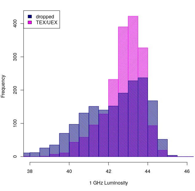
7
observables: 2.6 Black Hole Mass Measurements
 log peak = 0.597 × (log core − 40) + 44.156(erg/s). The analysis presented here relies on estimates of the central black
 hole mass for the jets in our sample. There are many different methods
A figure showing the correlation and fit is given in online Supple-
 of measuring the black hole mass ( BH ) in AGN. Reverberation
mental Figure B1.
 mapping, generally considered the most reliable method, uses the
 time delay between variations in the optical continuum and broad
 lines to give an estimate of the radius of the broad line region (BLR;
 Bentz 2015). The black hole mass is then derived from this time
 delay and the velocity of the gas in the BLR (as measured from the
2.5 The TEX and UEX Jet Samples width of the lines, Blandford & McKee 1982). Other methods take
 advantage of the observed correlations between BH and the galaxy
From the initial sample of nearly 7000 sources, we have selected
 bulge luminosity (which is an indicator of stellar mass, e.g. Marconi
those where the full SED had sufficient spectral coverage to reliably
 & Hunt 2003) as well as the correlation with the velocity dispersion
fit the synchrotron peak and return a value for the peak frequency
 of the stars in the galaxy (Ferrarese & Merritt 2000). Single-epoch
and luminosity. All SEDs were assessed visually for goodness of
 spectroscopy takes advantage of scaling relations between and
fit, without any a priori knowledge about their identity or type, sim-
 emission line luminosities (which are typically from large surveys,
ply based on being well-fit with an appropriate amount of spectral
 such as the Sloan Digital Sky Survey). This method only requires
coverage, following the same procedure as in M11. Generally, those
 a single observation to estimate , making it perhaps the most
that were eliminated lacked coverage over significant portions of the
 accessible method for large samples of AGN (e.g. Koss et al. 2017).
spectrum (e.g., no optical and/or X-ray) or could be reasonably fit
 We have attempted to exhaust the literature to compile BH mea-
by two or more very different SED shapes (often in these cases the
 surements for as many sources in the final sample as possible. Esti-
X-ray spectral index is unknown – see Appendix).
 mates of BH are available for 227 sources in the TEX sample (274
 A little more than one-third of the initial sample, or 2124 sources,
 sources for the combined TEX + UEX samples). In cases where there
remained after assessing the reliability of the broadband SED fit. Of
 are multiple reported values of BH , we take the average.
these, 1045 sources have estimates of the extended radio luminosity,
and we call this sample the "Trusted Extended" (TEX) sample, as in
M11. The TEX sample contains 575 FSRQs, 246 BL Lacs, 21 FR 2.7 Apparent Jet Speed Measurements
Is, and 41 FR IIs, and 162 sources of unknown object type. Another
1079 sources with good broadband SEDs only have upper limits With Very Long Baseline Interferometry (VLBI), it is possible to re-
on ext . We call this the "Unknown Extended" (UEX) sample as in solve small features in the flow near the base of the jet (e.g., Boccardi
M11. It contains 688 FSRQs, 242 BL Lacs, 0 FR Is, 1 FR IIs, and et al. 2017), which can be traced between observations to measure
148 sources of unknown type. All object types are based on either their proper motions, or apparent angular speeds ( ), which are typ-
the literature reference giving published nuclear fluxes (for radio ically on the order of mas/yr (e.g., Lister et al. 2019a; Jorstad et al.
galaxies, listed in Table 2) or from SIMBAD. All redshifts ( ) are 2017; Piner & Edwards 2018). When converted into the apparent
taken from SIMBAD and/or NED. In the TEX sample 103 sources speed ( app ) in units of the speed of light, sources are found to have
(169 in the UEX sample) have no redshift information available on superluminal speeds, up to about 80c, implying highly relativistic
SIMBAD/NED. In these cases a value of = 0.3 is assumed (≈ 10% flows. We have compiled a large catalog of all jets with proper motion
of the TEX sample, 16% of the UEX sample). This value was chosen measurements from published sources. Proper-motions monitoring
as it is roughly the transition from a nearby source to high-redshift programs often yield detections of multiple parsec-scale components
source (e.g. Bîrzan et al. 2020); however, none of our conclusions with different speeds (e.g. Lister et al. 2016). This could be due to
depend on this assumption, and we exclude these sources from plots an accelerating flow, differences in the flow speed over time, slight
with quantities (i.e., luminosities) that are strongly affected by the changes in the orientation angle, or variation in the angle of ejection
unknown redshift. A further discusson of these sources and their relative to the main jet direction (e.g. Lister et al. 2019a). These
properties and location in the peak − peak plane appears in the values typically tend to cluster around a characteristic speed. Dif-
Appendix. ferences can be on the order of the maximum speed (Lister et al.
 The properties of the TEX sample are given in Tables 6 and 7. 2013), although differences this large are rare. For this study, where
These include measurements of the black hole mass ( ) and multiple app values exist for a jet, we adopted the largest observed
apparent jet speed ( app ) which are described in the next sections. value. These are given in Tables 7 and B1 along with the appropri-
The radio properties of the TEX sample are given in Table 6, which ate reference. In all, 400 (289, 111) sources in the combined (TEX,
includes the source name in column 1, RA in column 2, DEC in UEX) catalog have a VLBI proper-motion measurement.
column 3, redshift in column 4, the 300-MHz extended luminosity
( ext ) in column 5, the 1.4 GHz core luminosity ( core ) in column
6, cross in column 7, the radio core dominance ( ) in column 8, 3 RESULTS AND DISCUSSION
apparent jet speed ( app ) in column 9 and the reference for app in
 3.1 Jet Power and the synchrotron peak − peak plane
column 10. Additional properties of the TEX sample are given in
Table 7, which includes the source name in column 1, object type Plots of peak versus peak are shown in Figure 3 for the TEX sample
(BLL, FSRQ, etc) in column 2, peak in column 3, peak in column (excluding those with missing redshift information), binned on ext .
4, BH in column 5 and the reference for BH in column 6. Column In all panels, BL Lac and FR I jets are shown as large circles with
7 gives the original sample ID with a letter code corresponding to black outlines, FSRQ and FR II are plotted as triangles, and sources
Table 1. of unknown type as small circles. All radio galaxies are enclosed in
 The properties of the UEX sample are available in online Supple- a red circle.
mental Table B1. With now nearly ten times the number of sources as in the original

 MNRAS 000, 1–20 (2021)

8 M. Keenan et al.

 48 0 ◦(1) log ergLext/s >43 0 ◦(1) 43 > log ergLext/s >42
 (2)◦ (2)◦
 46
log Lpeak(erg/s)

 0 0

 44
 42 BLL (13) BLL (62)
 FSRQ (233) FSRQ (250)
 45 ◦
 FR I (1) 45 ◦
 FR I (1)
 40 FR II (15)
 Unk (22)
 FR II (14)
 Unk (50)
 48 0 ◦(1) 42 > log ergLext/s >41 0 ◦(1) log ergLext/s

9

Table 6. TEX Radio Properties
 Source Name RA DEC Redshift ext core cross app Ref.
 – J2000 J2000 – erg/s erg/s Hz – c –
 (1) (2) (3) (4) (5) (6) (7) (8) (9) (10)

 WB 2359+1439 00 01 32.83 +14 56 08.13 0.3988 42.06 41.38 10.056 -0.88 ...
 PKS 2359-221 00 02 11.98 -21 53 09.86 ... 41.58 42.05 8.471 0.45 ...
 B3 0003+380 00 05 57.18 +38 20 15.15 0.2290 40.82 41.87 8.303 1.12 5.0950 c
 1Jy 0003-06 00 06 13.89 -06 23 35.34 0.3467 41.68 42.80 8.262 1.29 11.6540 t
 PKS 0007+10 00 10 31.01 +10 58 29.51 0.0900 39.96 40.22 9.207 -0.09 1.6560 o

 Table 6 is published in its entirety in the machine-readable format. A portion is shown here for guidance regarding its form and content. ext , core , and cross
are log10 values. The letters in column (10) denote the following references for app measurements: (a) Britzen et al. (2008) (b) Piner et al. (2007) (c) Lister
et al. (2016) (d) Lister et al. (2019a) (e) Vermeulen & Cohen (1994) (f) Piner & Edwards (2018) (g) Lister et al. (2009) (h) Piner et al. (2012) (i) Lister et al.
(2013) (j)Kellermann et al. (2004) (k) Jorstad et al. (2001) (l) Sudou & Iguchi (2011) (m) Jorstad et al. (2017) (n) Homan et al. (2001) (o) Frey et al. (2015) (p)
Piner et al. (2001) (q) Savolainen et al. (2006) (r) An et al. (2017) (s) Karamanavis et al. (2016) (t) Jorstad et al. (2005) (u) Jiang et al. (2002) (v) Gentile et al.
(2007) (w) Edwards & Piner (2002) (x) Lu et al. (2012) (y) Britzen et al. (2010) (z) Boccardi et al. (2016) (aa) Piner & Edwards (2004)

Table 7. TEX Broadband Properties
 Source Name Type peak peak BH Ref. Sample IDs
 – – erg/s Hz – –
 (1) (2) (3) (4) (5) (6) (7)

 PKS 0000-006 BLL 44.65 13.98 ... t
 IVS B0001-120 BLL 44.53 12.70 ... f,h
 PKS 0002-170 FSRQ 45.37 14.13 ... h,o
 NGC 315 FRII 41.76 12.42 9.0 p,n,i h,m,w
 TXS 0110+495 FSRQ 45.05 13.92 8.3 p e,f,h

 Table 7 is published in its entirety in the machine-readable format. A portion is shown here for guidance regarding its form and content. All measurements in
this table other than redshift are log10 values. The letters in column (6) denote the following references for measurements: (a) Barth et al. (2003) (b)
Bentz & Katz (2015) (c) Brotherton et al. (2016) (d) Chen et al. (2009) (e) Koss et al. (2017) (f) Kozłowski (2017) (g) Lewis & Eracleous (2006) (h) Liu et al.
(2006) (i) McKernan et al. (2010) (j) Pian et al. (2005) (k) Plotkin et al. (2011) (l) Ricci et al. (2017) (m) Savić et al. (2018) (n) van den Bosch (2016) (o) Wang
et al. (2004) (p) Woo & Urry (2002) (q) Woo et al. (2005) (r) Wu et al. (2002) (s) Wu et al. (2004) (t) Xie et al. (2005)

II" jets (quivalent to the "strong" jets of M11), and define the ‘strong at a certain power, but rather that type II jets are possible at any jet
zone’ as that bounded by peak > 1045 erg/s and peak < 1015 Hz. We power. This also matches recent discoveries of large numbers of FR
propose type I jets as those with intrinsically low-excitation optical II radio galaxies at low powers (Capetti et al. 2017b; Mingo et al.
spectra associated with low-efficiency accretion. In compliment to the 2019; Kozieł-Wierzbowska et al. 2020).
strong zone, we define a ‘weak zone’ of peak > 1015 Hz (see online The third observation is that for type I jets (those with peak > 1015
supplemental Figure B2); as this selects a population that is almost Hz) there appears to be an upper bound on the allowed jet power, as
entirely lineless BL Lac objects. Assuming that jets do de-beam like noted by the lack of these sources in the first panel of Figure 3 (with
the example paths shown, this definition of zones should avoid the ext > 1043 erg/s). As we will argue in Section 3.6, type I sources
mixture of jet types in the misaligned population at the bottom left likely correspond to inefficient accretion systems, and thus this upper
of the peak − peak plane. As we will show, the characteristics of bound could naturally arise from the observed upper limits on black
the jets in these two zones differ greatly. hole mass (109 − 1010 ) and the upper bound on the Eddington
 With the zones defined, we make three important observations. ratio (e.g., about 0.5% of Eddington) for the inefficient mode. The
First, that there are a substantial population of BL Lacs in the strong most powerful type I jets will be hosted by systems at these limits.
zone. The BL Lacs at low power and lower peak may be misaligned In comparison, the efficiently accreting systems that host type II jets,
versions of the more aligned BL Lacs in the weak zone proper (i.e, with the same range of black hole masses, will be able to reach jet
they are in the transition between blazars and radio galaxies). How- powers at least one order of magnitude higher.
ever, at the highest powers (i.e. BL Lacs shown as red circles at top
left of Figure 3), it is unlikely these are misaligned jets, as we would
expect to see the aligned counterparts (e.g. there are no high- peak
 3.2 The End of the Blazar Sequence
sources at these jet powers). We will return to the possibility that
many of the low-peak-frequency BL Lacs in the strong-jet zone are In Figure 4 we display peak versus peak for the combined UEX and
actually misidentified FSRQ (and argue that these should be consid- TEX samples (excluding those with missing redshift information).
ered type II jets) in section 3.5. Here BL Lacs and FR I are shown as large black circles, FSRQ and
 The second observation is that there are a sizable number of FSRQs FR II as red triangles, and unknown types as small blue points. Radio
with very low jet powers, seen as the blue filled triangles with ext < galaxies are further enclosed in circles, red for FR IIs and gray for FR
1041 erg/s at lower right in Figure 3. If broad-lined sources are Is. The theoretical de-beaming curves overlaid on the figure will be
always type II jets, this suggests that type I/II jets are not divided discussed in the next section. It is immediately obvious that with the

 MNRAS 000, 1–20 (2021)

10 M. Keenan et al.

 48
 0 ◦ (A) Strong Track
 (B) Weak Tracks
 47 0◦
 (C)
 ◦
 0
 46 0◦
 (E)
 45 (D)
log Lpeak(erg/s)

 0◦

 44
 43
 42 3C 264
 BLL
 45 ◦
 FSRQ
 41 FR I
 45 ◦
 Radio Galaxy Zone FR II
 40 Unk
 39
 11 12 13 14 15 16 17 18 19 20
 log νpeak(Hz)
Figure 4. Synchrotron peak luminosity ( peak ) versus peak frequency ( peak ) for the TEX and UEX samples combined, excluding those with missing redshift
information. Here BL Lacs and FR Is are plotted as black filled circles, and FSRQ and FR IIs as light red triangles. Radio galaxies are also circled in gray (FR
I) or red (FR II). The source 3C 264 is labeled as it is a topic of discussion in the main text. Paths (A), (B), (C), and (D) show theoretical de-beaming paths, as
discussed in the main text.

UEX sample included, there is a greater number of sources (nearly luminosity through an incorrectly assumed redshift.7 . We further
all BL Lacs) at high peak and high peak than in Figure 3. In the find that none of the UEX sources have an upper limit on log ext
combined sample there are 30 sources with peak > 1015 Hz and above 1043 erg/s. Thus a possible explanation for the high- peak ,
 peak > 1046 erg/s while in the TEX there are only 11. A handful high- peak sources preferentially appearing in the UEX sample is
of sources in or near this region have previously been described (e.g. that these are highly aligned type I jets with relatively low ext .
Padovani et al. 2003; Nieppola et al. 2006a; Padovani et al. 2012b; In such cases, the core spectrum will dominate down to very low
Giommi et al. 2012b; Cerruti et al. 2017), and our results appear to radio frequencies making an estimate of ext difficult given the large
agree with previous work showing that there is no ‘forbidden zone’ dynamic range between the highly beamed core and low-luminosity
at upper right in the peak − peak plane. extended emission (this is further supported by the range of radio
 core dominance discussed in Section 3.4).
 In previous work, some of the authors of this paper suggested
 Sources with high peak and high peak appear contrary to the
 that although the type I/II (weak/strong) jet divide and jet velocity
original blazar sequence, which implied an anti-correlation between
 gradients alters the original idea of the blazar sequence, there may
power and peak frequency, and more importantly, suggested that
 still be ‘sequence-like’ behavior within the two sub-populations, such
jets are mono-parametric. A deeper investigation of these particular
sources in our catalog is deferred to future work, but we can make
some observations from the data available. First, we can note that 7 Plots of 
 peak versus peak with a color scale on redshift for the full sample,
none of the forbidden-zone sources in our sample lack redshifts, and with a color scale on ext for the UEX sample (excluding those with miss-
and so their presence in this zone is not due to over-estimating the ing redshift information), are given in online supplemental Figures A4 and B3

MNRAS 000, 1–20 (2021)

11
 90 Abdo et al. 2009; Foschini et al. 2017). It is possible that the ‘down-
 80 Strong Zone Jets, log ergLext/s >43 43 > log ergLext/s >42
 νpeak =1013.22 ±0.03 Hz νpeak =1013.27 ±0.02 Hz sized’ low-power type II jets in general come from smaller black
 70
Number of Sources

 60 holes (see Section 3.6). As shown in Figure 5, we see that type II
 50 jets have a remarkably consistent distribution of synchroton peak
 40 frequencies over 4 orders of magnitude in jet power, as every bin has
 30 an average value of approximately peak = 1013.3 Hz (the average
 20 values and errors are obtained from a Gaussian fit, with exact values
 10 noted in the figure). Ghisellini et al. (2017), in a study of blazars
 300 detected by Fermi/LAT, similarly found that FSRQ do not appear to
 42 > log ergLext/s >41 log ergLext/s 43 43 > log ergLext/s >42
 L
 and show how the jet moves through the plane as it is misaligned
 νpeak =1015.62 ±0.19 Hz down to 45◦ . Track A shows the expected path for a single-velocity
Number of Sources

 20
 flow, as described for Figure 3, while tracks B, C, D, and E show
 15 example de-beaming paths for jets with velocity gradients using the
 10 decelerating flow model of Georganopoulos & Kazanas (2003) with
 different parameters. In all cases, the jet has a characteristic initial
 5 and final Lorentz factor (Γinit , Γfin ), and the deceleration occurs over
 0 a certain length scale ( decel , see Georganopoulos & Kazanas 2003,
 25 42 > log ergext/s >41 log ergLext/s 1015 Hz), binned on ext (as shown in the upper right corner). The shown here for reference. The parameters of track (B) have been cho-
 average values are shown as dashed vertical lines, with errors displayed as
 sen to explain the high- peak , high- peak sources that contradict the
 the horizontal bars. The average values of peak for these sources are found to
 original blazar sequence. If our interpretation is correct, we should
 remain constant with increasing ext . Note: there are no sources in the highest
 ext bin. see signs that these high-frequency, high-luminosity sources are very
 well aligned (see Section 3.4).
 The parameters of track (D) were chosen for the curve to pass
 that location in the peak − peak plane would be determined by jet near the few sources with relatively high peak and low peak , one of
 power (Georganopoulos et al. 2011; Meyer et al. 2012). The most which is the well-known source 3C 264, which hosts a superluminal
 straightforward test of this is to simply look at how type I and II jets optical jet (Meyer et al. 2015, labeled in Figure 4). The general lack
 behave in terms of the synchrotron peak frequency as a function of of sources in this region is important evidence for velocity gradients
 ext . in type I jets, since ‘simple’ (single-velocity flow) de-beaming of
 As previously noted, the FSRQs in our sample range from the the high-peak-frequeency BL Lacs should lead to a population of
 highest-power sources down to very low ext which appear to radio galaxies in this region. Although 3C 264 is nominally a radio
 match recent observations of low-luminosity sources with FR II galaxy, it is close to the ‘transition zone’ between radio galaxies and
 morphologies (Mingo et al. 2019) as well as the jets from smaller blazars with an orientation angle at or below 10 degrees (Archer et al.
 (106 − 107 ) black holes seen in narrow-line Seyfert galaxies (e.g. 2020). Thus it seems more likely that 3C 264 is a slightly misaligned

 MNRAS 000, 1–20 (2021)

12 M. Keenan et al.
 Track Γinit Γfin decel
 – – – cm 44
 B 26 3 1 × 1017
 C 15 3 5 × 1016
 D 6 3 2 × 1016 42

 log Lcore,1.4GHz(erg/s)
 E 10 3 1 × 1017
Table 8. The parameters describing the decelerating flow tracks in Figure 4.
 40
 Aligned
low-power analog to the higher-power jets that live above it in the OI = 1
 peak − peak plane. The source is well-studied enough for inclusion 38
likely only because it is very nearby ( = 0.02; =91 Mpc) and has
a prominent optical jet. It is found in both the 3C and 4C surveys; a Misaligned FSRQ
 logLext >44

 OI = 0 FR I
 44 >logLext >43.5
theoretical source at the same radio luminosity would drop out of the 36 43.5 >logLext >42.5
 FR II
 42.5 >logLext >41.5
3C survey beyond ≈ 0.03, and from the 4C survey beyond ≈ 0.08. Unk
 logLext 43.5) and lowest 40
 0.1
( ext < 41.5) power sources shows a decided shift (see histograms 39
in online Figure B4). The bulk of highest-power sources peak around 11 12 13 14 15 16 17 18 19 0.0
 c ∼ 0 and almost none have c > 1). The lowest-power sources logνpeak(Hz)
peak at c ∼0.5-1 and extend up to much higher values (core dom- Figure 8. The peak − peak plane with color scale based on the new ori-
inance of 2 or 3 is not unusual). The apparent ceiling on maximum entation indicator (OI) where a value of 1 corresponds to a highly aligned
 c for high-power jets is unlikely to be a selection effect against jet and a value of 0 to a misaligned jet. As expected, there is a noticeable
aligned sources: indeed, given a flux-limited sample high-power, gradient from aligned to misaligned as peak luminosity decreases. Their are
highly aligned sources will be over, not under-represented, due to indications that sources with intermediate synchrotron peak frequencies are
beaming effects. more misaligned. The original blazar sequence of Fossati et al., (1998) is
 In Figure 7, we plot c versus the core luminosity at 1.4 GHz denoted by the connected black diamonds.
( core ), with color representing ext for the TEX sample (excluding
those with missing redshift information). A thick black line is drawn
 on the jet power, with low-power sources having higher when
across the plot in the region of the most aligned sources. Here again
 fully aligned. For example, a very high-power jet (red sources in
we note that the maximum radio core dominance appears to depend
 Figure 7) with ≈ 0.5 could be nearly fully aligned, while a very
 low-power source (blue sources in Figure 7) with the same is well
8 Here we note the common usage of "low-peak", "intermediate-peak" and
 away from the most aligned sources of that power and in fact closer
"high-peak" BL Lacs, or LBLs, IBLs, and HBLs. The exact dividing line to the region of low-power radio galaxies (circled sources).
between classes varies slightly in the literature, but we adopt 1014.5 Hz < To roughly parameterize orientation, we assigned a value from 0
 peak < 1015.5 Hz for IBLs with HBLs and LBLs above and below this range, to 1 for each source relative to where the source lies with respect to
respectively. the parallel black lines drawn in Figure 7; we call this the "orientation

MNRAS 000, 1–20 (2021)

13
 48 70.0
indicator" (OI). An OI of 0 represents a source which is closer to
 LBL IBL HBL
the plane of the sky (i.e. at 90 degrees) and a value of 1 represents a
 47
source which is pointed along the line of sight. To better discriminate
between the bulk of sources, the lines are not absolutely outside the 46
entire population; outliers (sources outside of the black lines) were 10.0
simply truncated to a value of either 0 or 1 as appropriate. The 45

 log Lpeak(erg/s)
equation giving the OI value (before truncation) is 44

 βapp(c)
 OI = 0.077 core + 0.201 − 2.615
 43
where core is the power measured at 1.4 GHz and is the log
 42 1.0
ratio of the core to extended at 1.4 GHz.
 A binned version of the peak − peak plane for the TEX sample, 41
with a color scale corresponding to OI is shown in Figure 8. This
plot was created by separating the plane into 2D bins over peak 40
and peak , and taking the average value for the OI in each bin. Red 39
indicates that most of the sources which lie in that respective bin 11 12 13 14 15 16 17 18 19 0.1
are well-aligned, while blue indicates misaligned, according to the logνpeak(Hz)
scale shown at right. We find that the along the original blazar se-
quence (denoted by the connected black diamonds), most sources Figure 9. The peak − peak plane for all sources with measured app where
are well-aligned (red), as expected. We also find that for the type II we have taken an average over 2D bins in the plane. Red indicates fast speeds,
(strong zone) jets, sources become gradually more misaligned (blue) while blue indicates slow, as given by the (log) color scale at right. As
as peak decreases. The sources in the weak zone more complicated, expected, there is a noticeable gradient from aligned to misaligned among
likely due to a combination of the smaller sample size as well as sources at the left of the plane. We find that the maximum speed also de-
the mixed population at intermediate frequencies (the possibility of creases along the original blazar sequence (as indicated by the connected
‘intrinsic’ IBLs as mentioned earlier). However it does seem that black diamonds).
sources in the IBL region are more misaligned than those at the
highest peak frequencies. It is not clear if these more misaligned jets
are counterparts to the HBLs to the right in the plane or perhaps rare, and for a jet population over a range of orientations with similar
misaligned version of the high-frequency, high-luminosity sources intrinsic speeds, we would expect more aligned jets to have faster
which are largely absent from the TEX sample, as discussed previ- observed app .
ously. In general, the most misaligned sources are found in the lower VLBI studies have also shown that low-power jets have lower
left region of the peak − peak plane where radio galaxies reside, observed values of app (e.g., Kharb et al. 2010), so we also expect
as expected. Our results support the general picture where structured to see lower values of app in the type-I (weak jet) region of the
(weak/type I) jets follow largely horizontal movement through the peak − peak plane, relative to the type II (strong) zone, as well
 peak − peak plane. as the decrease in app with increasing orientation angle. Figure 9
 shows a binned average map (made in similar fashion to Figure 8)
 As a final comment on Figure 7, the fact that is highest in
 of the peak − peak plane with a color scale according to average
well-aligned, low-power jets may mean that these sources are less
 app , using all sources with measured app from the literature (400
likely to have detections of their extended radio emission. To detect
 total). While there are fewer high- peak sources with measured app ,
faint extended emission around a highly dominant core of 100-1000
 we find that jet speeds are lower in the region of type I blazars and
times the extended flux would require radio imaging which is highly
 radio galaxies, as expected.
sensitive and with high dynamic range, which is challenging. This
may explain why in general there are fewer low-power sources with
known ext compared to the most powerful FSRQ. More particularly,
 3.5 LBLs are type II Jets
it may explain the population of high-frequency, high-luminosity
sources in the UEX sample which seem to be largely missing from the Previous authors have suggested that some low-peaking BL Lacs
TEX sample, as previously discussed in Section 3.2. Future studies (LBLs, peak . 1015 Hz) are actually mis-identified FSRQ, where
with deep, high-dynamic-range radio imaging of these sources can the broad optical emission lines are present but overwhelmed by the
confirm this. We also note that our definition of OI is far from rigorous non-thermal jet emission (e.g. Georganopoulos & Marscher 1998;
and could be affected by selection effects, and the use of it here is Ghisellini et al. 2011a). This is supported by the observation that
meant to be more illustrative than conclusive. It is left to future work some BL Lac objects (including BL Lac itself) show broad lines
with more statistically complete samples to examine this in more when the jet is in a low state (e.g. Vermeulen et al. 1995; Corbett
detail. et al. 1996; Ghisellini et al. 2011b; D’Elia et al. 2015), while others
 Another way to look at orientation is through measurements of have features consistent with type II jets such as hotspots (Kollgaard
the apparent jet speed ( app , parameterized in units of ), which is et al. 1992; Murphy et al. 1993; Kharb et al. 2010) or the presence of
derived from observations of proper motions and has been measured a ‘big blue bump’ accretion disk signature in their broad-band SEDs.
for a large numbers of jets using very long-baseline radio interfer- In our SED fitting, a BBB component was added to an SED model fit
ometry (VLBI, e.g., Lister et al. 2019b). As app is a function of the when an obvious blue/UV bump was present in the data (regardless
bulk Lorentz factor (Γ) and the orientation , it can be used to put of any other source characteristics). The goal was mainly to improve
constraints on both. In particular, the maximum angle that a jet can the synchrotron peak fit by eliminating data from another emission
have can be found by letting the true jet speed equal unity. Although source, but it is also useful to see where jets with a BBB component
at very small orientation angles the apparent jet speed drops to zero fall in the peak − peak plane. In Figure 10 we plot peak vs. peak
because of extreme foreshortening, such highly aligned sources are again for the full UEX+TEX sample, and highlight those sources

 MNRAS 000, 1–20 (2021)