The Sensorium competition on predicting large-scale mouse primary visual cortex activity
←
→
Page content transcription
If your browser does not render page correctly, please read the page content below
The Sensorium competition on predicting
large-scale mouse primary visual cortex
activity
Konstantin F. Willeke1-3,*, , Paul G. Fahey4,5,*, , Mohammad Bashiri1-3 , Laura Pede3 , Max F. Burg1,3,6 , Christoph Blessing3 ,
Santiago A. Cadena1,3,6 , Zhiwei Ding4,5 , Konstantin-Klemens Lurz1-3 , Kayla Ponder4,5 , Taliah Muhammad4,5 , Saumil S.
Patel4,5 , Alexander S. Ecker3,7 , Andreas S. Tolias4,5,8 , and Fabian H. Sinz2-5
1
International Max Planck Research School for Intelligent Systems, University of Tübingen, Germany
arXiv:2206.08666v1 [q-bio.NC] 17 Jun 2022
2
Institute for Bioinformatics and Medical Informatics, University of Tübingen, Germany
3
Institute of Computer Science and Campus Institute Data Science, University of Göttingen, Germany
4
Department of Neuroscience, Baylor College of Medicine, Houston, TX, USA
5
Center for Neuroscience and Artificial Intelligence, Baylor College of Medicine, Houston, TX, USA
6
Institute for Theoretical Physics, University of Tübingen, Germany
7
Max Planck Institute for Dynamics and Self-Organization, Göttingen, Germany
8
Electrical and Computer Engineering, Rice University, Houston, USA
*,
Equal contributions
The neural underpinning of the biological visual system is Introduction
challenging to study experimentally, in particular as the neu-
ronal activity becomes increasingly nonlinear with respect Understanding how the visual system processes visual in-
to visual input. Artificial neural networks (ANNs) can serve a formation is a long standing goal in neuroscience. Neural
variety of goals for improving our understanding of this com- system identification approaches this problem in a quanti-
plex system, not only serving as predictive digital twins of tative, testable, and reproducible way by building accurate
sensory cortex for novel hypothesis generation in silico, but predictive models of neural population activity in response
also incorporating bio-inspired architectural motifs to pro- to arbitrary input. If successful, these models can serve as
gressively bridge the gap between biological and machine phenomenological digital twins for the visual cortex, allow-
vision. The mouse has recently emerged as a popular model
ing computational neuroscientists to derive new hypothe-
system to study visual information processing, but no stan-
ses about biological vision in silico, and enabling systems
dardized large-scale benchmark to identify state-of-the-art
models of the mouse visual system has been established. neuroscientists to test them in vivo (Bashivan et al., 2019;
To fill this gap, we propose the SENSORIUM benchmark com- Franke et al., 2021; Ponce et al., 2019; Walker et al., 2019).
petition. We collected a large-scale dataset from mouse pri- In addition, highly predictive models are also relevant to
mary visual cortex containing the responses of more than machine learning researchers who use them to bridge the
28,000 neurons across seven mice stimulated with thou- gap between biological and machine vision (Li et al., 2019,
sands of natural images, together with simultaneous behav- 2022; Safarani et al., 2021; Sinz et al., 2019).
ioral measurements that include running speed, pupil dila-
The work on predictive models of neural responses to vi-
tion, and eye movements. The benchmark challenge will
sual inputs has a long history that includes simple linear-
rank models based on predictive performance for neuronal
responses on a held-out test set, and includes two tracks for nonlinear (LN) models (Heeger, 1992a,b; Jones & Palmer,
model input limited to either stimulus only (SENSORIUM) or 1987), energy models (Adelson & Bergen, 1985), more
stimulus plus behavior (SENSORIUM+). We provide a start- general subunit/LN-LN models (Rust et al., 2005; Schwartz
ing kit to lower the barrier for entry, including tutorials, pre- et al., 2006; Touryan et al., 2005; Vintch et al., 2015), and
trained baseline models, and APIs with one line commands multi-layer neural network models (Lau et al., 2002; Lehky
for data loading and submission. We would like to see this et al., 1992; Prenger et al., 2004; Zipser & Andersen, 1988).
as a starting point for regular challenges and data releases, The deep learning revolution set new standards in predic-
and as a standard tool for measuring progress in large-scale tion performance by leveraging task-optimized deep con-
neural system identification models of the mouse visual sys- volutional neural networks (CNNs) (Cadena et al., 2019;
tem and beyond.
Cadieu et al., 2014; Yamins et al., 2014) and CNN-based ar-
chitectures incorporating a shared encoding learned end-to-
Correspondence: konstantin-friedrich.willeke@uni-tuebingen.de; end for thousands of neurons (Antolík et al., 2016; Bashiri
paul.fahey@bcm.edu; sinz@cs.uni-goettingen.de et al., 2021; Batty et al., 2016; Burg et al., 2021; Cadena
et al., 2019; Cowley & Pillow, 2020; Ecker et al., 2018;
Franke et al., 2021; Kindel et al., 2017; Klindt et al., 2017;
Lurz et al., 2020; McIntosh et al., 2016; Sinz et al., 2018;
Walker et al., 2019; Zhang et al., 2018).
Keywords. mouse visual cortex, system identification, neu- The core idea of a neural system identification approach to
ral prediction, natural images improve our understanding of an underlying sensory area is
Willeke*, Fahey* et al. | June 20, 2022 | 1–13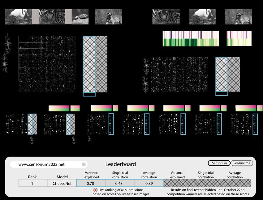
Fig. 1. A schematic illustration of the SENSORIUM competition. We will provide large-scale datasets of neuronal activity in the primary visual cortex of mice.
Participants of the competition will train models on pairs of natural image stimuli and recorded neuronal activity, in search for the best neural predictive model.

that models that explain more of the stimulus-driven variabil-                          ence (de Vries et al., 2019) are often not designed for a
ity may capture nonlinearities that previous low-parametric                             machine learning competition (consisting of only 118 nat-
models have missed (Carandini et al., 2005). Subsequent                                 ural images in addition to parametric stimuli and natural
analysis of high performing models, paired with ongoing                                 movies), and lacking benchmark infrastructure for measur-
in vivo verification, can eventually yield more complete                                ing predictive performance against a withheld test set.
principles of brain computation. This motivates continually                             To fill this gap, we created the SENSORIUM benchmark
improving our models to explain as much as possible of                                  competition to facilitate the search for the best predictive
the stimulus-driven variability and analyze these models to                             model for mouse visual cortex. We collected a large-scale
decipher principles of brain computations.                                              dataset from mouse primary visual cortex containing the
Standardized large-scale benchmarks are one approach                                    responses of more than 28,000 neurons across seven mice
to stimulate constructive competition between models com-                               stimulated with thousands of natural images, together with
pared on equal ground, leading to numerous seemingly                                    simultaneous behavioral measurements that include run-
small and incremental improvements that accumulate to                                   ning speed, pupil dilation, and eye movements. Benchmark
substantial progress. In machine learning and computer                                  metrics will rank models based on predictive performance
vision, benchmarks have been an important driver of in-                                 for neuronal responses on a held-out test set, and includes
novation in the last ten years. For instance, benchmarks                                two tracks for model input limited to either stimulus only
such as the ImageNetChallenge (Russakovsky et al., 2015)                                (SENSORIUM) or stimulus plus behavior (SENSORIUM+).
have helped jump start the revolution in artificial intelligence                        We also provide a starting kit to lower the barrier for en-
through deep learning.                                                                  try, including tutorials, pre-trained baseline models based
Similarly, neuroscience can benefit from more large-scale                               on published architectures (Klindt et al., 2017; Lurz et al.,
benchmarks to drive innovation and identify state-of-the-art                            2020), and APIs with one line commands for data loading
models. This is especially true in the mouse visual cortex,                             and submission. Our goal is to continue with regular chal-
which has recently emerged as a popular model system                                    lenges and data releases, as a standard tool for measuring
to study visual information processing, due to the wide                                 progress in large-scale neural system identification models
range of available genetic and light imaging techniques for                             of the mouse visual hierarchy and beyond.
interrogating large-scale neural activity.
Existing neuroscience benchmarks vary substantially in the
                                                                                        The SENSORIUM Competition
type of data, model organism, or goals of the contest (Cichy
et al., 2021; de Vries et al., 2019; Pei et al., 2021; Schrimpf                         The goal of the SENSORIUM 2022 competition is to identify
et al., 2018). For example, the Brain-Score benchmark                                   the best models for predicting a large number of sensory
(Schrimpf et al., 2018) ranks task -pretrained models that                              neural responses to arbitrary natural stimuli. The start of
best match areas across primate visual ventral stream and                               the competition is accompanied by the public release of a
other behavioral data, but rather than providing neuronal                               training dataset for refining model performance (for more
training data, participants are expected to design objec-                               details, see Data and Fig. 2), including two animals for
tives, learning procedures, network architectures, and input                            which a competition test set has been withheld.
data that result in representations that are predictive of                              For the held-out competition test set, the recorded neu-
the withheld neural data. The Algonauts challenge (Cichy                                ronal responses will not be (and have never been) publicly
et al., 2021) competition ranks neural predictive models of                             released. The test set images are divided into two exclu-
human brain activity recorded with fMRI in visual cortex in                             sive groups: live and final test. Performance metrics (see
response to natural images and videos. Additionally, large                              Metrics) computed on the live test images will be used to
data releases such as the extensively annotated dataset                                 maintain a public leaderboard on our website throughout
in mouse visual cortex from Allen Institute for Brain Sci-                              the submission period, while the performance metrics on

2                                                                                                                           Willeke*, Fahey* et al.   |   SENSORIUM 2022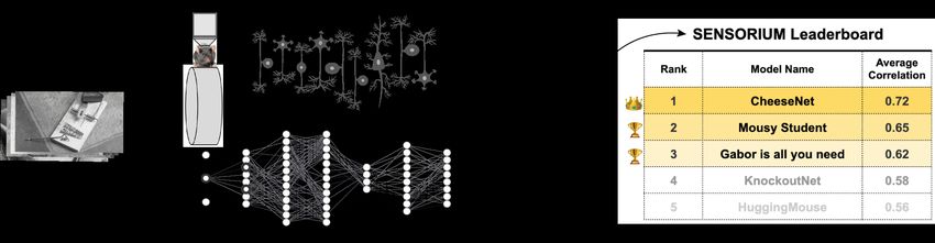
Fig. 2. Overview of the data and the competition structure. a, Detailed view of the data format of a single recording used for the SENSORIUM track. The
data consists of training images (N≈5000) and the associated scalar neuronal activity of each neuron. Furthermore, there are two test sets, the live and final sets,
consisting of 100 images, shown 10 times each to the animal. The neuronal responses to both test sets are withheld. b, SENSORIUM+ track. Same as in (a) but for
this track, the behavioral variables are also provided. c, overview of the seven recordings in our dataset. The pre-training recordings are not part of the competition
evaluation, but they can be used to improve model performance. The live test set images are also contained in the pre-training recordings (see blue frame in all
panels), along with the neuronal responses. Thus, we refer to this set as the public test set. In summary: the live and public test set have the same images, but
different neurons. d, the live test set scores are displayed on the live leaderboard. The final test set scores will be validated and revealed after the submissions close.

the final test images will be used to identify the winning                                   includes the natural image stimuli but not the behavioral
entries, and will only be revealed after the submission pe-                                  variables (Fig. 2a). Thus, the focus of this challenge is
riod has ended (Fig. 2d). By separating the live test and                                    the stimulus-driven responses, treating other correlates of
final test set performance metrics, we are able to provide                                   neural variability, such as behavioral state, as noise. This
feedback on performance on the live test set to participants                                 track resembles most of the current efforts in the commu-
wishing to submit updated predictions over the course of                                     nity (Schrimpf et al., 2018) to identify stimulus-response
the competition (up to the limit of one submission per day),                                 functions without any additional information about the brain
while protecting the validity of the final test set from overfit-                            and behavioral state.
ting over multiple submissions.                                                              SENSORIUM+ In the second challenge, participants will
The competition has two tracks, SENSORIUM and                                                predict neuronal activity of 7,538 neurons in response to
SENSORIUM+ , predicting two datasets with the same stim-                                     200 unique natural images of our competition live test and
uli, but from two different animals and with differing model                                 final test image sets. In this case, the data provided in-
inputs, as detailed in the following.                                                        cludes both the natural image stimuli and the accompanying
SENSORIUM. In the first challenge, participants have to                                      behavioral variables (Fig. 2b, see Sec. below). As a signifi-
predict neuronal activity of 7,776 neurons in response to                                    cant part of response variability correlates with the animal’s
200 unique natural images of our competition live test and                                   behavior and internal brain state (Niell & Stryker, 2010;
final test image sets. The data provided for the test set                                    Reimer et al., 2014; Stringer et al., 2019), their inclusion

Willeke*, Fahey* et al.   |   SENSORIUM 2022                                                                                                                                  3
in the modeling process can result in models that capture        these images as live test set. Furthermore, the competition
single trial neural responses more accurately (Bashiri et al.,   recordings contain 10 repetitions of 100 additional natural
2021; Franke et al., 2021).                                      test images that were randomly intermixed during the ex-
                                                                 periment. These test images are only present in the two
Data                                                             competition recordings. The responses to these images will
                                                                 also be withheld and used to determine the winner of the
The competition dataset was designed with the goal of            competition after submissions are closed (Fig. 2a,b). We
comparing neural predictive models that capture neuronal         refer to these images as our final test set. By providing both
responses r ∈ Rn of n neurons as a function fθ (x) of either     live and final test scoring, participants receive the benefit
only natural image stimuli x ∈ Rh×w (image height,width),        of iterative feedback while avoiding overfitting on the final
or as a function fθ (x, b) of both natural image stimuli and     scoring metrics.
behavioral variables b ∈ Rk . We provide k = 5 variables:        In our first competition track (SENSORIUM, Fig. 2a), we
locomotion speed, pupil size, instantaneous change of pupil      withhold the behavioral variables, such that only the natu-
size (second order central difference), and horizontal and       ral images can be used to predict the neuronal responses.
vertical eye position. See Fig. 2 for an overview of the         For the other competition track (SENSORIUM+, Fig. 2b), as
dataset.                                                         well as the five pre-training recordings recordings, we are
Natural images. We sampled natural images from Im-               releasing all the behavioral variables. For the pre-training
ageNet (Russakovsky et al., 2015). The images were               recordings, we are also releasing the order of the presented
cropped to fit a monitor with 16:9 aspect ratio, converted to    images as shown to the animal, but we withhold this infor-
gray scale, and presented to mice for 500 ms, preceded by        mation in the competition datasets, to discourage partic-
a blank screen period between 300 and 500 ms (Fig. 2a,b)         ipants from learning neuronal response trends over time.
Neuronal responses. We recorded the response of exci-            Lastly, we are releasing the anatomical locations of the
tatory neurons in layer 2/3 of the right primary visual cortex   recorded neurons for all datasets.
in awake, head-fixed, behaving mice using calcium imaging.       The complete corpus of data is available to download 1 .
Neuronal activity was extracted and accumulated between
50 and 550 ms after each stimulus onset using a boxcar
window.                                                          Performance Metrics
Behavioral variables. During imaging, mice were head-            Across the two benchmark tracks, three metrics of pre-
mounted over a cylindrical treadmill, and an eye camera          dictive accuracy will be automatically and independently
captured changes in the pupil position and dilation. Behav-      computed for the 100 live test set images and 100 final test
ioral variables were similarly extracted and accumulated         set images, for which the ground-truth neuronal responses
between 50 and 550 ms after each stimulus onset using a          are withheld. Due to their nature, not all three metrics will
boxcar window.                                                   be computed for both tracks of the competition and only
Dataset. Our complete corpus of data comprises seven             one of the three metrics on the final test set will be used for
recordings in seven animals (Fig. 2c), which in total contain    independently ranking the submissions to the two bench-
the neuronal activity of more than 28,000 neurons to a total     mark tracks. See Materials and Methods for further details
of 25,200 unique images, with 6,000–7,000 image presen-          and formulae.
tations per recording. We report a conservative estimate of      Correlation to Average We calculate the correlation to
the number of neurons present in the data, due to dense          average ρav of 100 model predictions to the withheld, ob-
recording planes in our calcium imaging setup, which leads       served mean neural response across 10 repeated presen-
to single neurons producing multiple segmented units by          tations of the same stimulus. This metric will be computed
appearing in multiple recording planes. Fig. 2c shows the        for both the SENSORIUM and SENSORIUM+ tracks to fa-
uncorrected number with a total of 54,569 units.                 cilitate comparison. Correlation to average on the final
Five of the seven recordings, which we refer to as pre-          test set will serve as the ultimate ranking score in the
training recordings (Fig. 2c, right), are provided solely for    SENSORIUM track to determine competition winners.
training and model generalization. The pre-training record-      Fraction of Explainable Variance Explained (FEVE)
ings are not included in the competition performance met-        While the Correlation to average is a common metric, it is
rics. They contain 5,000 single presentations of natural         insensitive to affine transformations of either the neuronal
images which are randomly intermixed with 10 repetitions         response or predictions. Thus, we also compute FEVE to
of 100 natural images, and all corresponding neuronal re-        measure how well the model accounts for stimulus-driven
sponses. The 100 repeated images and responses serve             (i.e. explainable) variations in neuronal response (Cadena
as a public test set for each recording.                         et al., 2019). This metric computes the ratio between the
In the two remaining recordings, our competition record-         variance explained by the model and the explainable vari-
ings (Fig. 2c, left), the mice were also presented with 5,000    ance in the neural responses. The explainable variance
single presentations of training stimuli as well as the pub-     accounts for only the stimulus-driven variance and ignores
lic test images. However, during the contest, we withhold        the trial-to-trial variability in responses (see Materials and
the responses to the public test images and use them for
the live leaderboard during the contest. We thus refer to           1 http://sensorium2022.net/

4                                                                                           Willeke*, Fahey* et al.   |   SENSORIUM 2022
Baseline performance on held out test data
Live test set Final test set
Single Trial Correlation Single Trial Correlation
Competition track FEVE FEVE
Correlation to Average Correlation to Average
CNN Baseline .274 .513 .433 .287 .528 .439
SENSORIUM
LN Baseline .197 .363 .222 .207 .377 .232
CNN Baseline .374 .571 - .384 .578 -
SENSORIUM+
LN Baseline .257 .373 - .266 .385 -
Table 1. Performance of the baseline models on both tracks of the competition. For the start of our competition, we are providing baseline scores for two models in each
competition track. The main score which will determine the winner of the competition is written in boldface. Note that the fraction of explainable variance explained (FEVE) is
calculated on a subset of neurons with an explainable variance larger than 15% (See section Materials and Methods for details). Furthermore, FEVE can not be computed
for the SENSORIUM+ track (see Materials and Methods).
Methods for details). This metric will be computed for full dataset 2 . The following material is included:
SENSORIUM but not SENSORIUM+ , due to the lack of
repeated trials with the exactly same behavior fluctuations • Code to download our complete corpus of data and
necessary to estimate the noise ceiling with FEVE. For to load it for model fitting.
numerical stability, we compute the FEVE only for neurons
• A visual guide to the properties of the dataset, to give
with an explainable variance larger than 15% (See section
neuroscientists as well as non-experts an overview
Materials and Methods for details).
of the scale and all properties of the data.
Single Trial Correlation Lastly, to measure how well mod-
els account for trial-to-trial variations we compute the single • Code to re-train the baselines, as well as checkpoints
trial correlation ρst between predictions and single trial neu- to load our pre-trained baselines.
ronal responses, without averaging across repeats. This
metric will be computed for both the SENSORIUM and • Ready-to-use code to generate a submission file to
SENSORIUM+ tracks to facilitate comparison. Single trial enter the competition.
correlation on the final test set will serve as the ultimate
By facilitating ease of use, we hope that our competition
ranking score in the SENSORIUM+ track to determine com-
will be of use to both computational neuroscientists and
petition winners.
machine learning practitioners alike to apply their knowl-
edge and model-building skills on an interesting biological
problem.
Baseline
To establish baselines for our competition, we trained simple
Discussion
linear-nonlinear models (LN Baseline) as well as a state-of-
the-art convolutional neural network (CNN Baseline, Lurz Here, we introduce the SENSORIUM competition to find
et al. (2020)) models for both competitions. The resulting the best predictive model for the mouse primary visual
model performances can be found in Table 1. We trained a cortex, with the accompanying release of a large-scale
single model (based on one random seed) for each com- dataset of more than 28,000 neurons across seven mice
petition track and model type. We trained each model on and their activity in response to natural stimuli. We hope
the training set of the respective competition track only, not that this competition and public benchmark infrastructure
utilizing the pre-training scans to facilitate reproducibility. will serve as a catalyst for both computational neuroscien-
An example of how to utilize the pre-training scans can be tists and machine learning practitioners to advance the field
found in our “starting kit”. Further improvement in predic- of neuro-predictive modeling. Our broader goal is to con-
tive performance can be made by using model ensembles, tinue to populate the underlying benchmark infrastructure
which can lead to a performance gain of 5-10%. For further with additional future iterations of dataset releases, regular
details on the model architecture and training procedure, challenges, and additional metrics.
refer to the Materials and Methods section. As is the case for benchmarks in general, by converging
in this first iteration on a specific dataset, task, and evalu-
ation metric in order to facilitate constructive comparison,
Additional Resources SENSORIUM 2022 also becomes limited to the scope of
those choices. In particular, we opted for simplicity for the
We are releasing our “starting kit” that contains the com-
plete code to fit our baseline models as well as explore the 2 https://github.com/sinzlab/sensorium
Willeke*, Fahey* et al. | SENSORIUM 2022 5first competition hosted on our platform in order to appeal to under-emphasize the contribution of the stimulus-driven
a broader audience across the computational neuroscience component. In addition, upper bounds are often challeng-
and machine learning communities. A priori, it is not clear ing to define for these metrics.
how well the best performing models of this competition More broadly, a potential concern about predictive modeling
would transfer to a broader or more naturalistic setting – in general is that the models with the highest predictive per-
for example, predicting freely moving animals’ neural ac- formance generally lack interpretability of how they achieve
tivity to arbitrary naturalistic videos in an ethologically rele- their performance due to their complexity, which limits scien-
vant color spectrum. Having established our benchmarking tific insight. However, we think that the converse is equally
framework, we plan to alleviate the constraints imposed problematic: a simpler model that is interpretable but poorly
by the data by extending future challenges in a number of predicts neural activity, in particular to natural stimuli, would
dimensions, such as: also be unhelpful. We believe that a fruitful avenue for
gaining insight into the brain’s functional processing is to
• including cortical layers beyond L2/3 and other areas
iteratively combine both approaches: developing new mod-
in mouse visual cortex beyond V1
els to push the state-of-the-art predictive performance and
• replacing static image stimuli with dynamic movie at the same time extracting knowledge by simplifying com-
stimuli in order to better capture the temporal evolu- plex models or by analyzing models post-hoc. For exam-
tion of representation and/or simulation ple, Burg et al. (2021) simplified the state-of-the-art model
by Cadena et al. (2019) showing that divisive normaliza-
• replacing grayscale visual stimuli with coverage of tion accounts for most but not all of its performance; and
both UV- and green-sensitive cone photoreceptors Ustyuzhaninov et al. (2022) simplified and analyzed the rep-
resentations learned by a high-performing complex model
• increasing the number of animals and recordings revealing a combinatorial code of non-linear computations
in the test set beyond one per track to emphasize in mouse V1.
generalization across animals and brain states
Additionally, high performing predictive models may also
• moving beyond passive viewing of visual stimuli benefit computational neuroscientists by serving as digital
by incorporating decision making into the stimulus twins, creating an in silico environment in which hypotheses
paradigm may be developed and refined before returning to the in
vivo system for validation (Bashivan et al., 2019; Franke
• including different or multiple sensory domains (e.g., et al., 2021; Ponce et al., 2019; Walker et al., 2019). This
auditory, olfactory, somatosensory, etc) and motor approach can not only enable exhaustive experiments that
areas are otherwise technically infeasible in vivo, but also limit
cost and ethical burden by decreasing the number of ani-
• recording neural responses with different techniques
mals required to pursue scientific questions.
(e.g., electrophysiology) that emphasize different pop-
Taken together, we believe that predictive models have be-
ulation sizes and spatiotemporal resolution
come an important tool for neuroscience research. In our
• recording neural responses in different animal mod- view, systematically benchmarking and improving these
els, such as non-human primates. models along with the development of accurate metrics will
be of great benefit to neuroscience as a whole. We there-
• inverting model architecture to reconstruct visual in- fore invite the research community to join the benchmarking
put from neural responses. effort by participating in the challenge, and by contributing
new datasets and metrics to our benchmarking system. We
Similarly, selection of appropriate metrics for model per-
would like to cast the challenge of understanding informa-
formance is also challenging as, despite considerable
tion processing in the brain as a joint endeavor in which
progress in this domain (Haefner & Cumming, 2008;
we engage together as a whole community, iteratively re-
Pospisil & Bair, 2020; Schoppe et al., 2016), there is not
defining what is the state-of-the-art in predicting neural
yet a consensus metric for evaluating predictive models of
activity and leveraging models to pursue the question of
the brain. Ideally, such a metric would appropriately handle
how the brain makes sense of the world.
different sources of variability present in neural responses
and have a calibrated upper bound (i.e., where perfect pre-
diction of the stimulus-driven component receives a perfect Acknowledgments. KKL is funded by the German Federal
score). Metrics such as the fraction of explainable variance Ministry of Education and Research through the Tübin-
explained (FEVE, Cadena et al. (2019)) partially address gen AI Center (FKZ: 01IS18039A). FHS is supported by
this issue, but focus on the mean and variance are not ap- the Carl-Zeiss-Stiftung and acknowledges the support of
plicable in settings when no two trials with identical inputs the DFG Cluster of Excellence “Machine Learning – New
exist, for example when the input includes uncontrolled Perspectives for Science”, EXC 2064/1, project number
behavioral variables. On the other hand, likelihood-based 390727645. This work was supported by an AWS Machine
metrics can reflect the entire conditional response distribu- Learning research award to FHS. MB and SAC were sup-
tion, but can be sensitive to the choice of noise model and ported by the International Max Planck Research School
6 Willeke*, Fahey* et al. | SENSORIUM 2022for Intelligent Systems. This project has received funding was increased exponentially as a function of depth from the
from the European Research Council (ERC) under the Eu- surface according to:
ropean Union’s Horizon Europe research and innovation
programme (Grant agreement No. 101041669). P = P0 × e(z/Lz ) (1)
This research was supported by National Institutes of
Here P is the laser power used at target depth z, P0 is the
Health (NIH) via National Eye Insitute (NEI) grant RO1-
power used at the surface (not exceeding 19 mW), and Lz
EY026927, NEI grant T32-EY002520, National Institute of
is the depth constant (220 µm). The greatest laser output of
Mental Health (NIMH) and National Institute of Neurological
55 mW was used at approximately 245 µm from the surface,
Disorders and Stroke (NINDS) grant U19-MH114830, and
with most scans not requiring more than 40 mW at similar
NINDS grant U01-NS113294. This research was also sup-
depths.
ported by National Science Foundation (NSF) NeuroNex
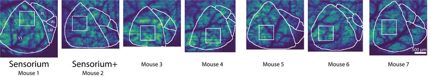
grant 1707400. The content is solely the responsibility of The craniotomy window was leveled with regards to the ob-
the authors and does not necessarily represent the official jective with six degrees of freedom. Pixel-wise responses
views of the NIH, NEI, NIMH, NINDS, or NSF. from an ROI spanning the cortical window (>3000 x 3000
µm, 0.2 px/µm, between 200-220 µm from surface, >3.9
This research was also supported by the Intelligence Ad-
Hz) to drifting bar stimuli were used to generate a sign
vanced Research Projects Activity (IARPA) via Department
map for delineating visual areas (Garrett et al., 2014). Area
of Interior/Interior Business Center (DoI/IBC) contract no.
boundaries on the sign map were manually annotated. Our
D16PC00003, and with funding from the Defense Advanced
target imaging site was a 630 x 630 x 45 um volume (an-
Research Projects Agency (DARPA), Contract No. N66001-
teroposterior x mediolateral x radial depth) in L2/3, within
19-C-4020. The US Government is authorized to reproduce
the boundaries of primary visual cortex (VISp, Supp.Fig. 1).
and distribute reprints for governmental purposes notwith-
The released scans contained 10 planes, with 5 µm inter-
standing any copyright annotation thereon. The views and
plane distance in depth, and were collected at 7.98 Hz.
conclusions contained herein are those of the authors and
Each plane is 630 × 630 µm (252 × 252 pixels, 0.4 px/µm).
should not be interpreted as necessarily representing the of-
The most superficial plane in each volume ranged from
ficial policies or endorsements, either expressed or implied,
approximately 190 - 220 µm from the surface. This high
of IARPA, DoI/IBC, DARPA, or the US Government.
spatial sampling in z results in the nearest plane no more
AUTHOR CONTRIBUTIONS that 2.5 µm from the theoretical best imaging plane for
KFW: Conceptualization, Methodology, Data curation, Validation, Software, Formal each neuron, but also results in redundant masks for many
Analysis, Analysis design, Writing - Original Draft & Editing, Visualization, Project
administration; PGF: Conceptualization, Methodology, Data acquisition, Data cu- neurons in adjacent planes.
ration, Visualization, Writing - Original Draft & Editing; MB: Conceptualization, Movie of the animal’s eye and face was captured throughout
Methodology, Software, Analysis design, Writing - Original Draft & Editing; LP: Con-
ceptualization, Software, Writing - Original Draft & Editing; MFB: Conceptualiza- the experiment. A hot mirror (Thorlabs FM02) positioned
tion, Software, Writing - Original Draft & Editing; CB: Software, Analysis design ; between the animal’s left eye and the stimulus monitor was
SAC:Conceptualization, Methodology, Software, Analysis design, Writing - Original
Draft & Editing; ZD: Data acquisition, Data curation; KKL:Methodology, Software, used to reflect an IR image onto a camera (Genie Nano
Writing - Original Draft & Editing; KP: Data acquisition, Data curation; TM: Data ac- C1920M, Teledyne Dalsa) without obscuring the visual stim-
quisition, Data curation; SSP: Data acquisition; AE: Conceptualization, Supervision,
Writing - Review & Editing, Funding acquisition; AST: Supervision, Data acquisition, ulus. The position of the mirror and camera were manually
Writing - Review & Editing, Funding acquisition; FHS: Conceptualization, Supervi- calibrated per session and focused on the pupil. Field
sion, Writing - Review & Editing, Funding acquisition;
of view was manually cropped for each session. For five
pre-training scans, the field of view contained the superior,
frontal, and inferior portions of the facial silhouette as well
Materials and Methods
as the left eye in its entirety, ranging from 664-906 pixels
Neurophysiological experiments. All procedures were height x 1014-1113 pixels width at 20 Hz. In two remaining
approved by the Institutional Animal Care and Use Com- competition scans, the field of view contained only the left
mittee of Baylor College of Medicine. Seven mice (Mus eye in its entirety, 282-300 pixels height x 378-444 pixels
musculus, 5 females, 2 males) expressing GCaMP6s in width at 20 Hz. Frame times were time stamped in the be-
excitatory neurons via Slc17a7-Cre and Ai162 transgenic havioral clock for alignment to the stimulus and scan frame
lines (recommended and generously shared by Hongkui times. Video was compressed using Labview’s MJPEG
Zeng at Allen Institute for Brain Science; JAX stock 023527 codec with quality constant of 600 and stored in an AVI file.
and 031562, respectively) were anesthetized and a 4 mm Light diffusing from the laser during scanning through the
craniotomy was made over the visual cortex of the right pupil was used to capture pupil diameter and eye move-
hemisphere as described previously (Froudarakis et al., ments. A DeepLabCut model (Mathis et al., 2018) was
2014; Reimer et al., 2014). trained on 17 manually labeled samples from 11 animals to
Mice were head-mounted above a cylindrical treadmill label each frame of the compressed eye video (intraframe
and calcium imaging was performed using Chameleon Ti- only H.264 compression, CRF:17) with 8 eyelid points and
Sapphire laser (Coherent) tuned to 920 nm and a large 8 pupil points at cardinal and intercardinal positions. Pupil
field of view mesoscope (Sofroniew et al., 2016) equipped points with likelihood >0.9 (all 8 in 92-98% of frames) were
with a custom objective (excitation NA 0.6, collection NA fit with the smallest enclosing circle, and the radius and
1.0, 21 mm focal length). Laser power after the objective center of this circle was extracted. Frames with < 3 pupil
Willeke*, Fahey* et al. | SENSORIUM 2022 7points with likelihood >0.9 ( 5.5 standard deviations from shown and repeated 10 times each (total 7000 trials). Each the mean in any of the three parameters (center x, center image was presented for 500 ms, preceded by a blank y, radius,
constrained non-negative matrix factorization, then decon-       Gaussian readout (Lurz et al., 2020), which simplifies the
volved to extract estimates of spiking activity, within the      regression problem considerably. The Gaussian read-
CAIMAN pipeline (Giovannucci et al., 2019). Cells were           out learns the parameters of a 2D Gaussian distribution
further selected by a classifier trained to separate somata      N (µn , Σn ). The mean µn in the readout feature space
versus artifacts based on segmented cell masks, resulting        thus represents the center of a neuron’s receptive field in
in exclusion of 9.1% of masks.                                   image space, whereas Σn refers to the uncertainty of the
Functional and behavioral signals were upsampled to 100          receptive field position. During training, a location of height
Hz by nearest neighbor interpolation, then all points within     and width in the core output tensor in each training step
a boxcar window from 50 - 550 ms after stimulus onset            is sampled, for every image and neuron. Given a large
were averaged to produce the trial value. The mirror mo-         enough initial Σn to ensure gradient flow, the uncertainty
tor coordinates of the centroid of each mask was used to         about the readout location Σn is decreasing during training,
assign anatomical coordinates relative to each other and         showing that the estimates of the mean location µn be-
the experimenter’s estimate of the pial surface. Notably,        comes more and more reliable. At inference time (i.e. when
centroid positional coordinates do not carry information         evaluating our model), we set the readout to be determinis-
about position relative to the area boundaries, or relative      tic and to use the fixed position µn . In parallel to learning
to neurons in other scans. Multiple masks corresponding          the position, we learned the weights of the weight tensor of
to the intersection of a single neuron’s light footprint with    the linear regression of size c per neuron. To learn the posi-
multiple imaging planes were detected by iteratively as-         tions µn , we made use of the retinotopic organization of V1
signing edges between units with anatomical coordinates          by coupling the recorded cortical 2d-coordinates pn ∈ R2
within 80 µm euclidean distance and with correlation over        of each neuron with the estimation of the receptive field
0.9 between the full duration deconvolved traces after low       position µn of the readout. We achieved this by learning
pass filtering with a Hann window and downsampling to            the common function µn = f (pn ), a randomly initialized
1 Hz. The total number of unique neurons per scan was            linear fully connected MLP of size 2-30-2, shared by all
estimated by the number of unconnected components in             neurons.
the resulting graph per scan.
                                                                 Shifter network We employed a free viewing paradigm
                                                                 when presenting the visual stimuli to the head-fixed mice.
Model architecture. Our best performing model of the
                                                                 Thus, the RF positions of the neurons with respect to the
mouse primary visual cortex is a convolutional neural net-
                                                                 presented images had considerable trial to trial variability
work (CNN) model, which is split into two parts: the core
                                                                 following any eye movements. We informed our model
and the readout (Cadena et al., 2019; Franke et al., 2021;
                                                                 of the trial dependent shift of the neurons receptive fields
Lurz et al., 2020; Sinz et al., 2018). First, the core com-
                                                                 due to eye movement by shifting µn , the model neuron’s
putes latent features from the inputs. Then, the readout is
                                                                 receptive field center, using the estimated eye position (see
learned per neuron and maps the output of the rich core
                                                                 section Neurophysiological experiments above for details
feature space to the neuronal responses via regularized
                                                                 of estimating the pupil center). We passed the estimated
regression. This architecture reflects the inductive bias of
                                                                 pupil center through a MLP, called shifter network, a three
a shared feature space across neurons. In this view, each
                                                                 layer fully connected network with n = 5 hidden features,
neuron represents a linear combination of features realized
                                                                 followed by a tanh nonlinearity, that calculates the shift in
at a certain position in the visual field, known as as the
                                                                 ∆x and ∆y of the neurons receptive field in each trial. We
receptive field.
                                                                 then added this shift to the µn of each neuron.
Representation/Core      We based our work on the models
                                                                 Input of behavioral parameters    During each presentation
of Lurz et al. (2020) and Franke et al. (2021), which are able
                                                                 of a natural image, the pupil size, instantaneous change
to predict the responses of a large population of mouse V1
                                                                 of pupil size, and the running speed of the mouse was
neurons with high accuracy. In brief, we modeled the core
                                                                 recorded. For the SENSORIUM+ track, we have used these
as a four-layer CNN, with 64 feature channels per layer. In
                                                                 behavioral parameters to improve the model’s predictivity.
each layer, a 2d-convolution is followed by batch normaliza-
                                                                 Because these behavioral parameters have nonlinear mod-
tion and an ELU nonlinearity (Clevert et al., 2015; Ioffe &
                                                                 ulatory effects, we decided to appended them as separate
Szegedy, 2015). Except for the first layer, all convolutions
                                                                 images to the input images as new channels (Franke et al.,
are depth-separable (Chollet, 2017). The latent features
                                                                 2021), such that each new channel simply consisted of the
that the core computed for a given input are then forwarded
                                                                 scalar for the respective behavioral parameter recorded
to the readout.
                                                                 in a particular trial, transformed into stimulus dimension.
Readout   To get the scalar neuronal firing rate for each        This enabled the model to predict neural responses as a
neuron, we computed a linear regression between the core         function of both visual input and behavior.
output tensor of dimensions x ∈ Rw×h×c (width, height,
channels) and the linear weight tensor w ∈ Rc×w×h , fol-         Model training. We first split the unique training images
lowed by an ELU offset by one (ELU+1), to keep the re-           into the training and validation set, using a split of 90% to
sponse positive. We made use of the recently proposed            10%, respectively. Subsequently, we isotropically down-

Willeke*, Fahey* et al.   |   SENSORIUM 2022                                                                                  9
sampled all images to a resolution of 36 × 64 px (h × w), re- Both metrics are restricted in that they are point estimates,
sulting in a resolution of 0.53 pixels per degree visual angle. and as such do not measure the correctness of the entire
Furthermore, we normalized Input images as well behav- probability distribution that the model has learned. Instead,
ioral traces and standardized the target neuronal activities, they only measure the correctness of the first moment of
using the statistics of the training trials of each record- this distribution, i.e. the mean.
ing. Then, we trained our networks with the training set by Correlation to Average Given a neuron’s response rij to
1 Pm (i) − r (i) log r̂ (i) ,
minimizing the Poisson loss m i=1 r̂ image i and repeat j and predictions oi , the correlation is
where m denotes the number of neurons, r̂ the predicted computed between the predicted responses and the aver-
neuronal response and r the observed response. After age neuronal response ri to the ith test image (averaged
each epoch, i.e. full pass through the training set, we cal- across repeated presentations of the same stimulus):
culated the correlation between predicted and measured
neuronal responses on the validation set and averaged P
(r̄i − r̄)(oi − ō)
it across all neurons. If the correlation failed to increase ρav = corr(rav , oav ) = pP i , (3)
2 2
P
during for five consecutive epochs, we stopped the training i i − r̄)
(r̄ i (oi − ō)
and restored the model to its state after the best performing PJ
epoch. Then, we either decreased the learning rate by where r̄i = J1 j=1 rij is the average response across J
a factor of 0.3 or stopped training altogether, if the num- repeats, r̄ is the average response across all repeats and
ber of learning-rate decay steps was reached (n=4 decay images, and ō is the average prediction across all repeats
steps). We optimized the network’s parameters using the and images.
Adam optimizer (Kingma & Ba, 2015). Furthermore, we Fraction Explainable Variance Explained For N = I · J
performed an exhaustive hyper-parameter selection using is the total number of trials from I images and J repeats
Bayesian search on a held-out dataset. All parameters and per image:
hyper-parameters regarding model architecture and train-
1
− oi )2 − σε2
P
ing procedure can be found in our sensorium repository N i,j (rij
FEVE = 1 − , (4)
(see Code Availability). Var[r] − σε2
where Var[r] is the total response variance computed
LN model. Our LN model has the same architecture as
across all N trials and σε2 = Ei [Varj [r|x]] is the observation
our CNN model, but with all non-linearities removed except
noise variance computed as the average variance across
the final ELU+1 nonlinearity, thus turning the CNN model
responses to repeated presentations of the stimulus x. As
effectively into a fully linear model followed by a single
the bounds of FEVE are [−∞, 1], neurons with low explain-
output non-linearity. We performed a search for the best
able variance can have a substantially negative FEVE value
architectural parameters on a held-out dataset and arrived
and thus bias the population average. We therefore restrict
at a model with three layers, and otherwise unchanged
the calculation of the FEVE to all units with an explainable
parameters as compared to the CNN model. The addition
variance larger than 15%, in line with previous literature
of the shifter network, behavioral parameters, as well as the
(Cadena et al., 2019).
whole training procedure, was identical to the CNN model.
Single Trial Correlation To measure how well models ac-
Metrics. We chose to evaluate the models via two metrics count for trial-to-trial variations we compute correlation ρst
that are commonly used in neuroscience but differ in their between predictions and single trial neuronal responses,
properties and focus: Correlation and Fraction of Explain- without averaging across repeats.
able Variance Explained (FEVE).
Since correlation is invariant to shift and scale of the pre- P
− r̄)(oij − ō)
i,j (rij
dictions, it does not reward a correct prediction of the ab- ρst = corr(rst , ost ) = qP , (5)
2 2
P
solute value of the neural response but rather the neuron’s i,j (rij − r̄) i,j (oij − ō)
relative response changes. It is bound to [−1, 1] and thus
easily interpretable. However, without accounting for the where r̄ is the average response across all repeats and
unexplainable noise in neural responses, the upper bound images, and ō is the average prediction across all repeats
of 1 cannot be reached, which can be misleading. and images.
FEVE, on the other hand, does correct for the unexplain-
able noise and provides provides an estimate for the upper Code and data availability. Our competition website
bound of stimulus-driven activity. This measure is equiva- can be reached under http://sensorium2022.
lent to variance explained (R2 ) corrected for observation net/. There, the complete datasets are available
noise. However, since its bounds are [−∞, 1], models can for download. Our coding framework uses gen-
be arbitrarily bad. If the model predicts the constant mean eral tools like PyTorch, Numpy, scikit-image, mat-
of the target responses, FEVE will evaluate to 0. In the case plotlib, seaborn, DataJoint, Jupyter, Docker, CAIMAN,
of single-trial model evaluation in the SENSORIUM+ track, DeepLabCut, Psychtoolbox, Scanimage, and Kuber-
FEVE is not possible to compute, as it requires stimulus netes. We also used the following custom libraries
trial repeats to estimate the unexplainable variability. and code: neuralpredictors (https://github.
10 Willeke*, Fahey* et al. | SENSORIUM 2022com/sinzlab/neuralpredictors) for torch-based Heeger, D. J. (1992b). Normalization of cell responses in cat striate cortex. Vis. Neurosci., 9(2),
181–197.
custom functions for model implementation, nnfabrik Ioffe, S., & Szegedy, C. (2015). Batch normalization: accelerating deep network training by reduc-
(https://github.com/sinzlab/nnfabrik) for au- ing internal covariate shift. In Proceedings of the 32nd International Conference on Machine
Learning, ICML’15, (pp. 448–456). JMLR.org.
tomatic model training pipelines, and sensorium for utili- Jones, J. P., & Palmer, L. A. (1987). The two-dimensional spatial structure of simple receptive
ties (https://github.com/sinzlab/sensorium). fields in cat striate cortex. J. Neurophysiol., 58(6), 1187–1211.
Kindel, W. F., Christensen, E. D., & Zylberberg, J. (2017). Using deep learning to reveal the neural
code for images in primary visual cortex.
References Kingma, D. P., & Ba, J. (2015). Adam: A method for stochastic optimization. In Y. Bengio, &
Y. LeCun (Eds.) 3rd International Conference on Learning Representations, ICLR 2015, San
Adelson, E. H., & Bergen, J. R. (1985). Spatiotemporal energy models for the perception of Diego, CA, USA, May 7-9, 2015, Conference Track Proceedings.
motion. J. Opt. Soc. Am., 2(2), 284–299. Kleiner, M. B., Brainard, D. H., Pelli, D. G., Ingling, A., & Broussard, C. (2007). What’s new in
Antolík, J., Hofer, S. B., Bednar, J. A., & Mrsic-flogel, T. D. (2016). Model constrained by visual psychtoolbox-3. Perception, 36, 1–16.
hierarchy improves prediction of neural responses to natural scenes. PLoS Comput. Biol., (pp. Klindt, D. A., Ecker, A. S., Euler, T., & Bethge, M. (2017). Neural system identification for large
1–22). populations separating “what” and “where”. In Advances in Neural Information Processing
Bashiri, M., Walker, E., Lurz, K.-K., Jagadish, A., Muhammad, T., Ding, Z., Ding, Z., Tolias, A., & Systems, (pp. 4–6).
Sinz, F. (2021). A flow-based latent state generative model of neural population responses to Lau, B., Stanley, G. B., & Dan, Y. (2002). Computational subunits of visual cortical neurons
natural images. Adv. Neural Inf. Process. Syst., 34. revealed by artificial neural networks. Proceedings of the National Academy of Sciences,
Bashivan, P., Kar, K., & DiCarlo, J. J. (2019). Neural population control via deep image synthesis. 99(13), 8974–8979.
Science (New York, N.Y.), 364(6439). Lehky, S., Sejnowski, T., & Desimone, R. (1992). Predicting responses of nonlinear neurons in
Batty, E., Merel, J., Brackbill, N., Heitman, A., Sher, A., Litke, A., Chichilnisky, E. J., & Paninski, L. monkey striate cortex to complex patterns. The Journal of Neuroscience, 12(9), 3568–3581.
(2016). Multilayer network models of primate retinal ganglion cells. URL https://doi.org/10.1523/jneurosci.12-09-03568.1992
Brainard, D. H. (1997). The psychophysics toolbox. Spat. Vis., 10(4), 433–436. Li, Z., Brendel, W., Walker, E. Y., Cobos, E., Muhammad, T., Reimer, J., Bethge, M., Sinz, F. H.,
Burg, M. F., Cadena, S. A., Denfield, G. H., Walker, E. Y., Tolias, A. S., Bethge, M., & Ecker, Pitkow, X., & Tolias, A. S. (2019). Learning from brains how to regularize machines.
A. S. (2021). Learning divisive normalization in primary visual cortex. PLOS Computational Li, Z., Caro, J. O., Rusak, E., Brendel, W., Bethge, M., Anselmi, F., Patel, A. B., Tolias, A. S.,
Biology, 17(6), e1009028. & Pitkow, X. (2022). Robust deep learning object recognition models rely on low frequency
Cadena, S. A., Denfield, G. H., Walker, E. Y., Gatys, L. A., Tolias, A. S., Bethge, M., & Ecker, A. S. information in natural images.
(2019). Deep convolutional models improve predictions of macaque v1 responses to natural Lurz, K.-K., Bashiri, M., Willeke, K., Jagadish, A. K., Wang, E., Walker, E. Y., Cadena, S. A.,
images. PLOS Computational Biology, 15(4), e1006897. Muhammad, T., Cobos, E., Tolias, A. S., Ecker, A. S., & Sinz, F. H. (2020). Generalization in
Cadieu, C. F., Hong, H., Yamins, D. L. K., Pinto, N., Ardila, D., Solomon, E. A., Majaj, N. J., & data-driven models of primary visual cortex. In Proceedings of the International Conference
DiCarlo, J. J. (2014). Deep neural networks rival the representation of primate IT cortex for for Learning Representations (ICLR), (p. 2020.10.05.326256).
core visual object recognition. PLoS Comput. Biol., 10(12), e1003963. Mathis, A., Mamidanna, P., Cury, K. M., Abe, T., Murthy, V. N., Mathis, M. W., & Bethge, M. (2018).
Carandini, M., Demb, J. B., Mante, V., Tolhurst, D. J., Dan, Y., Olshausen, B. A., Gallant, J. L., & DeepLabCut: markerless pose estimation of user-defined body parts with deep learning. Nat.
Rust, N. C. (2005). Do we know what the early visual system does? J. Neurosci., 25(46), Neurosci., 21(9), 1281–1289.
10577–10597. McIntosh, L. T., Maheswaranathan, N., Nayebi, A., Ganguli, S., & Baccus, S. A. (2016). Deep
Chollet, F. (2017). Xception: Deep learning with depthwise separable convolutions. In learning models of the retinal response to natural scenes. Adv. Neural Inf. Process. Syst.,
Proceedings - 30th IEEE Conference on Computer Vision and Pattern Recognition, CVPR 29(Nips), 1369–1377.
2017. Niell, C. M., & Stryker, M. P. (2010). Modulation of visual responses by behavioral state in mouse
Cichy, R. M., Dwivedi, K., Lahner, B., Lascelles, A., Iamshchinina, P., Graumann, M., Andonian, visual cortex. Neuron, 65(4), 472–479.
A., Murty, N. A. R., Kay, K., Roig, G., & Oliva, A. (2021). The algonauts project 2021 challenge: Pei, F., Ye, J., Zoltowski, D., Wu, A., Chowdhury, R. H., Sohn, H., O’Doherty, J. E., Shenoy, K. V.,
How the human brain makes sense of a world in motion. Kaufman, M. T., Churchland, M., Jazayeri, M., Miller, L. E., Pillow, J., Park, I. M., Dyer, E. L.,
URL https://arxiv.org/abs/2104.13714 & Pandarinath, C. (2021). Neural latents benchmark ’21: Evaluating latent variable models of
Clevert, D.-A., Unterthiner, T., & Hochreiter, S. (2015). Fast and accurate deep network learning neural population activity.
by exponential linear units (ELUs). URL https://arxiv.org/abs/2109.04463
Cowley, B., & Pillow, J. (2020). High-contrast "gaudy" images improve the training of deep neural Pelli, D. G. (1997). The VideoToolbox software for visual psychophysics: transforming numbers
network models of visual cortex. In H. Larochelle, M. Ranzato, R. Hadsell, M. Balcan, & H. Lin into movies. Spat. Vis., 10(4), 437–442.
(Eds.) Advances in Neural Information Processing Systems 33, (pp. 21591–21603). Curran Ponce, C. R., Xiao, W., Schade, P. F., Hartmann, T. S., Kreiman, G., & Livingstone, M. S. (2019).
Associates, Inc. Evolving images for visual neurons using a deep generative network reveals coding principles
de Vries, S. E. J., Lecoq, J. A., Buice, M. A., Groblewski, P. A., Ocker, G. K., Oliver, M., Feng, D., and neuronal preferences. Cell, 177(4), 999–1009.e10.
Cain, N., Ledochowitsch, P., Millman, D., Roll, K., Garrett, M., Keenan, T., Kuan, L., Mihalas, Pospisil, D. A., & Bair, W. (2020). The unbiased estimation of the fraction of variance explained
S., Olsen, S., Thompson, C., Wakeman, W., Waters, J., Williams, D., Barber, C., Berbesque, by a model.
N., Blanchard, B., Bowles, N., Caldejon, S. D., Casal, L., Cho, A., Cross, S., Dang, C., Dol- Prenger, R., Wu, M. C.-K., David, S. V., & Gallant, J. L. (2004). Nonlinear V1 responses to natural
beare, T., Edwards, M., Galbraith, J., Gaudreault, N., Gilbert, T. L., Griffin, F., Hargrave, P., scenes revealed by neural network analysis. Neural Netw., 17(5-6), 663–679.
Howard, R., Huang, L., Jewell, S., Keller, N., Knoblich, U., Larkin, J. D., Larsen, R., Lau, Reimer, J., Froudarakis, E., Cadwell, C. R., Yatsenko, D., Denfield, G. H., & Tolias, A. S. (2014).
C., Lee, E., Lee, F., Leon, A., Li, L., Long, F., Luviano, J., Mace, K., Nguyen, T., Perkins, Pupil fluctuations track fast switching of cortical states during quiet wakefulness. Neuron,
J., Robertson, M., Seid, S., Shea-Brown, E., Shi, J., Sjoquist, N., Slaughterbeck, C., Sulli- 84(2), 355–362.
van, D., Valenza, R., White, C., Williford, A., Witten, D. M., Zhuang, J., Zeng, H., Farrell, C., Russakovsky, O., Deng, J., Su, H., Krause, J., Satheesh, S., Ma, S., Huang, Z., Karpathy, A.,
Ng, L., Bernard, A., Phillips, J. W., Reid, R. C., & Koch, C. (2019). A large-scale standard- Khosla, A., Bernstein, M., Berg, A. C., & Fei-Fei, L. (2015). ImageNet large scale visual
ized physiological survey reveals functional organization of the mouse visual cortex. Nature recognition challenge. Int. J. Comput. Vis., 115(3), 211–252.
Neuroscience, 23(1), 138–151. Rust, N. C., Schwartz, O., Movshon, J. A., & Simoncelli, E. P. (2005). Spatiotemporal elements of
URL https://doi.org/10.1038/s41593-019-0550-9 macaque v1 receptive fields. Neuron, 46(6), 945–956.
Ecker, A. S., Sinz, F. H., Froudarakis, E., Fahey, P. G., Cadena, S. A., Walker, E. Y., Cobos, E., Safarani, S., Nix, A., Willeke, K., Cadena, S., Restivo, K., Denfield, G., Tolias, A., & Sinz, F. (2021).
Reimer, J., Tolias, A. S., & Bethge, M. (2018). A rotation-equivariant convolutional neural Towards robust vision by multi-task learning on monkey visual cortex. Adv. Neural Inf. Process.
network model of primary visual cortex. Syst., 34, 739–751.
Franke, K., Willeke, K. F., Ponder, K., Galdamez, M., Muhammad, T., Patel, S., Froudarakis, E., Schoppe, O., Harper, N. S., Willmore, B. D. B., King, A. J., & Schnupp, J. W. H. (2016). Measuring
Reimer, J., Sinz, F., & Tolias, A. S. (2021). Behavioral state tunes mouse vision to ethological the performance of neural models. Frontiers in Computational Neuroscience, 10.
features through pupil dilation. bioRxiv. URL https://doi.org/10.3389/fncom.2016.00010
URL https://www.biorxiv.org/content/early/2021/10/13/2021.09.03. Schrimpf, M., Kubilius, J., Hong, H., Majaj, N. J., Rajalingham, R., Issa, E. B., Kar, K., Bashivan,
458870 P., Prescott-Roy, J., Geiger, F., Schmidt, K., Yamins, D. L. K., & DiCarlo, J. J. (2018). Brain-
Froudarakis, E., Berens, P., Ecker, A. S., Cotton, R. J., Sinz, F. H., Yatsenko, D., Saggau, P., score: Which artificial neural network for object recognition is most brain-like?
Bethge, M., & Tolias, A. S. (2014). Population code in mouse V1 facilitates readout of natural URL https://doi.org/10.1101/407007
scenes through increased sparseness. Nat. Neurosci., 17(6), 851–857. Schwartz, O., Pillow, J. W., Rust, N. C., & Simoncelli, E. P. (2006). Spike-triggered neural charac-
Garrett, M. E., Nauhaus, I., Marshel, J. H., & Callaway, E. M. (2014). Topography and areal terization. J. Vis., 6(4), 484–507.
organization of mouse visual cortex. J. Neurosci., 34(37), 12587–12600. Sinz, F., Ecker, A. S., Fahey, P., Walker, E., Cobos, E., Froudarakis, E., Yatsenko, D., Pitkow,
Giovannucci, A., Friedrich, J., Gunn, P., Kalfon, J., Brown, B. L., Koay, S. A., Taxidis, J., Najafi, F., X., Reimer, J., & Tolias, A. (2018). Stimulus domain transfer in recurrent models for large
Gauthier, J. L., Zhou, P., Khakh, B. S., Tank, D. W., Chklovskii, D. B., & Pnevmatikakis, E. A. scale cortical population prediction on video. In Advances in Neural Information Processing
(2019). CaImAn: An open source tool for scalable calcium imaging data analysis. Elife, 8, Systems 31.
e38173. Sinz, F. H., Pitkow, X., Reimer, J., Bethge, M., & Tolias, A. S. (2019). Engineering a less artificial
Haefner, R., & Cumming, B. (2008). An improved estimator of variance explained in the presence intelligence. Neuron, 103(6), 967–979.
of noise. In D. Koller, D. Schuurmans, Y. Bengio, & L. Bottou (Eds.) Advances in Neural URL https://doi.org/10.1016/j.neuron.2019.08.034
Information Processing Systems, vol. 21. Curran Associates, Inc. Sofroniew, N. J., Flickinger, D., King, J., & Svoboda, K. (2016). A large field of view two-photon
URL https://proceedings.neurips.cc/paper/2008/file/ mesoscope with subcellular resolution for in vivo imaging. Elife, 5, e14472.
2ab56412b1163ee131e1246da0955bd1-Paper.pdf Stringer, C., Pachitariu, M., Steinmetz, N., Reddy, C. B., Carandini, M., & Harris, K. D. (2019).
Heeger, D. J. (1992a). Half-squaring in responses of cat striate cells. Vis. Neurosci., 9(5), 427– Spontaneous behaviors drive multidimensional, brainwide activity. Science, 364(6437).
443. Touryan, J., Felsen, G., & Dan, Y. (2005). Spatial structure of complex cell receptive fields mea-
Willeke*, Fahey* et al. | SENSORIUM 2022 11You can also read