On age of air climatologies and trends - The impact of sulfur hexafluoride (SF6) sinks
←
→
Page content transcription
If your browser does not render page correctly, please read the page content below
Research article
Atmos. Chem. Phys., 22, 1175–1193, 2022
https://doi.org/10.5194/acp-22-1175-2022
© Author(s) 2022. This work is distributed under
the Creative Commons Attribution 4.0 License.

                  The impact of sulfur hexafluoride (SF6 ) sinks
                     on age of air climatologies and trends
           Sheena Loeffel1 , Roland Eichinger2,1,5 , Hella Garny1,2 , Thomas Reddmann3 , Frauke Fritsch1,2 ,
                                Stefan Versick4 , Gabriele Stiller3 , and Florian Haenel3
                 1 Institut für Physik der Atmosphäre, Deutsches Zentrum für Luft- und Raumfahrt (DLR),
                                                   Oberpfaffenhofen, Germany
                        2 Institut für Meteorologie, Ludwig Maximilians Universität, Munich, Germany
         3 Institute for Meteorology and Climate Research, Karlsruhe Institute of Technology, Karlsruhe, Germany
              4 Steinbuch Centre for Computing (SCC), Karlsruhe Institute of Technology, Karlsruhe, Germany
               5 Department of Atmospheric Physics, Faculty of Mathematics and Physics, Charles University,

                                                     Prague, Czech Republic
                                 Correspondence: Sheena Loeffel (sheena.loeffel@dlr.de)

                                  Received: 24 March 2021 – Discussion started: 23 April 2021
                     Revised: 19 November 2021 – Accepted: 22 November 2021 – Published: 24 January 2022

      Abstract. Mean age of air (AoA) is a common diagnostic for the strength of the stratospheric overturning cir-
      culation in both climate models and observations. AoA climatologies and AoA trends over the recent decades of
      model simulations and proxies derived from observations of long-lived tracers do not agree. Satellite observa-
      tions show much older air than climate models, and while most models compute a clear decrease in AoA over the
      last decades, a 30-year time series from measurements shows a statistically nonsignificant positive trend in the
      Northern Hemisphere extratropical middle stratosphere. Measurement-based AoA derivations are often founded
      on observations of the trace gas sulfur hexafluoride (SF6 ), a fairly long-lived gas with a near-linear increase in
      emissions during recent decades. However, SF6 has chemical sinks in the mesosphere that are not considered in
      most model studies. In this study, we explicitly compute the chemical SF6 sinks based on chemical processes
      in the global chemistry climate model EMAC (ECHAM/MESSy Atmospheric Chemistry). We show that good
      agreement between stratospheric AoA in EMAC and MIPAS (Michelson Interferometer for Passive Atmospheric
      Sounding) is reached through the inclusion of chemical SF6 sinks, as these sinks lead to a strong increase in the
      stratospheric AoA and, therefore, to a better agreement with MIPAS satellite observations. Remaining larger dif-
      ferences at high latitudes are addressed, and possible reasons for these differences are discussed. Subsequently,
      we demonstrate that the AoA trends are also strongly influenced by the chemical SF6 sinks. Under consideration
      of the SF6 sinks, the AoA trends over the recent decades reverse sign from negative to positive. We conduct sen-
      sitivity simulations which reveal that this sign reversal does not result from trends in the stratospheric circulation
      strength nor from changes in the strength of the SF6 sinks. We illustrate that even a constant SF6 destruction rate
      causes a positive trend in the derived AoA, as the amount of depleted SF6 scales with increasing SF6 abundance
      itself. In our simulations, this effect overcompensates for the impact of the accelerating stratospheric circulation
      which naturally decreases AoA. Although various sources of uncertainties cannot be quantified in detail in this
      study, our results suggest that the inclusion of SF6 depletion in models has the potential to reconcile the AoA
      trends of models and observations. We conclude the study with a first approach towards a correction to account
      for SF6 loss and deduce that a linear correction might be applicable to values of AoA of up to 4 years.

Published by Copernicus Publications on behalf of the European Geosciences Union.
1176                                                                         S. Loeffel et al.: The impact of SF6 sinks on AoA

1   Introduction                                                    pling of in situ observations can be the reason for the above-
                                                                    mentioned trend discrepancies. Birner and Bönisch (2011)
The Brewer–Dobson circulation (BDC) describes the strato-           as well as Bönisch et al. (2011) argued that differences in
spheric transport circulation, consisting of the mean over-         the changes between the deep and the shallow BDC branch
turning circulation of air ascending in the tropical pipe, mov-     can possibly explain these. Ploeger et al. (2015) showed that
ing poleward and descending in the extratropics (Brewer,            the residual circulation transit time cannot explain the AoA
1949; Dobson and Massey, 1956), as well as isentropic mix-          trends and that the integrated effect of mixing (which is cou-
ing. A good measure to diagnose this transport circulation is       pled to residual circulation changes; see Garny et al., 2014)
the age of stratospheric air (AoA), which is defined as the         is crucial. Moreover, Stiller et al. (2017) could explain a
mean transport time of an air parcel from its entry into the        hemispheric asymmetry by a shift of subtropical transport
stratosphere (or from the surface) to any point therein (Hall       barriers. In a study based on a chemistry transport model,
and Plumb, 1994; Waugh and Hall, 2002). In general circu-           Kouznetsov et al. (2020) showed that changes in SF6 -derived
lation models (GCMs), AoA is commonly represented by an             apparent AoA over 1 decade are highly influenced by the SF6
inert tracer with a strictly linear temporally increasing sur-      sink and can even turn positive. However, a comprehensive
face mixing ratio and is calculated as the corresponding time       understanding of the magnitude of the individual effects on
lag between the local mixing ratio and the mixing ratio at a        the AoA trend depending on altitude and latitude is still miss-
reference point (Hall and Plumb, 1994). The same method             ing.
can be applied to real long-lived tracers with a linear trend in        SF6 sinks lead to an older apparent AoA (see, e.g., Waugh
tropospheric concentration, and AoA has been derived, for           and Hall, 2002, and Kouznetsov et al., 2020) as well as
example, from balloon-borne in situ measurements of sul-            shorter lifetimes. Leedham Elvidge et al. (2018) evaluated
fur hexafluoride (SF6 ) (Andrews et al., 2001; Engel et al.,        AoA from several tracers including SF6 and found clear dif-
2009, 2017). This trace gas is particularly suitable for these      ferences between them, indicating a shorter SF6 lifetime than
studies, as it is stable in the troposphere and stratosphere and    previously assumed. The strongest chemical SF6 removal re-
its tropospheric concentrations have increased nearly linearly      actions take place in the mesosphere; the most important re-
over recent decades. Along with observations of other trace         moval processes are electron attachment and UV photoly-
gases, these measurements form a long-term dataset of obser-        sis, but these processes have not yet been precisely quan-
vationally based AoA restricted to the Northern Hemisphere          tified. Ravishankara et al. (1993) estimated an SF6 lifetime
midlatitudes that covers more than 40 years. A near-global          of 3200 years, and Reddmann et al. (2001) found a lifetime
dataset of AoA covering 10 years from 2002 to 2012 was de-          of between 400 and 10000 years, depending on the assumed
rived in Stiller et al. (2012), Haenel et al. (2015), and Stiller   loss reactions and electron density. A more recent model
et al. (2017), who retrieved SF6 distributions from MIPAS           study by Kovács et al. (2017), who used the Whole Atmo-
(Michelson Interferometer for Passive Atmospheric Sound-            sphere Community Climate Model (WACCM) to determine
ing) satellite observations, but these cover a much shorter         the atmospheric lifetime of SF6 , reported a mean SF6 life-
time period.                                                        time of 1278 years, and Ray et al. (2017) provided a range
   Observations and model simulations of AoA often dis-             between 580 and 1400 years based on in situ measurements
agree. AoA derived from observations is mainly older than           in the stratospheric polar vortex. The most recent model
simulated AoA (see, e.g., SPARC, 2010, and Dietmüller               study of Kouznetsov et al. (2020), who performed simula-
et al., 2018), and the AoA trend over recent decades even           tions of tracer transport with a chemical transport model,
differs in sign between observations and models. While most         shows an SF6 lifetime ranging between 600 and 2900 years.
climate models show a clear decrease in AoA over time               Due to these uncertainties and the complex computation of
(see, e.g., Butchart and Scaife, 2001, Garcia et al., 2011, and     the chemical reactions, most model studies do not consider
Eichinger et al., 2019), consistent with the simulated accel-       any SF6 sinks for the calculation of AoA from SF6 mixing
eration of the BDC in the course of climate change (see, e.g.,      ratios. This can explain why most climate models generally
Garcia and Randel, 2008), the time series of the observations       show younger stratospheric air than observations, in partic-
presented in the studies by Engel et al. (2009), Ray et al.         ular within the polar vortices (e.g., Haenel et al., 2015; Ray
(2014), and Engel et al. (2017) show a (statistically non-          et al., 2017).
significant) positive trend (note that Ray et al., 2014, also           In the present study, we apply the chemistry climate model
shows negative balloon AoA trends in the lower extratropi-          EMAC (ECHAM MESSy Atmospheric Chemistry; Jöckel
cal stratosphere). This discrepancy has been addressed in nu-       et al., 2010; Jöckel et al., 2016) with the aim of understand-
merous studies. For example, Garcia et al. (2011) showed            ing the effects of SF6 sinks on tracer-derived AoA and its
that, due to the concave growth rate of tropospheric SF6 con-       long-term trends. Specifically, for the first time, we calcu-
centrations, the AoA trends derived from an SF6 tracer are          late the effect of the sinks on the long-term trend in SF6 -
smaller than the trends derived from a synthetic, linearly          derived AoA and quantify how this effect is modulated by
growing AoA tracer (also after accounting for the nonlin-           circulation changes (recent climate change), specified model
ear growth rates of SF6 ). They noted that the sparse sam-          dynamics, or by changes in the abundance of relevant species

Atmos. Chem. Phys., 22, 1175–1193, 2022                                              https://doi.org/10.5194/acp-22-1175-2022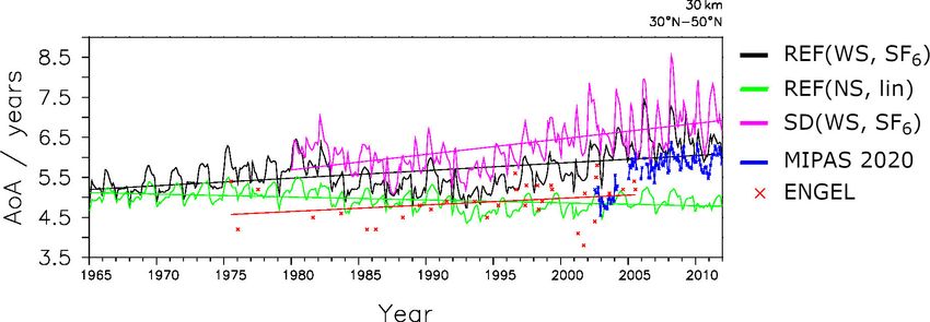
S. Loeffel et al.: The impact of SF6 sinks on AoA                                                                                1177

for SF6 chemistry. Furthermore, we analyze the contribu-              2.2   Submodel SF6
tion of the SF6 sinks themselves on the long-term trend in
SF6 -based AoA. As an outlook, we thereupon provide first             The submodel SF6 is used to calculate the lifetime of SF6 by
thoughts on how to apply an AoA correction to observations            explicitly accounting for the sinks of SF6 in the mesosphere.
taking SF6 sinks into account. The chemistry climate model            The submodel is operationally available for all users in
uses the second version of the Modular Earth Submodel Sys-            MESSy from version 2.54.0 onward. The calculation method
tem (MESSy2) to link multi-institutional computer codes. In           for this is based on the reaction scheme of Reddmann et al.
our simulations, we employed the MESSy submodel “SF6”                 (2001). The most important reaction involved in the chemical
which explicitly calculates SF6 sinks based on physical pro-          degradation of SF6 , namely electron attachment, is included
cesses (based on Reddmann et al., 2001), rather than on crude         in the SF6 submodel. The configuration of the submodel al-
parameterizations. We apply a correction for the nonlinear            lows for a simple exponential profile for the electron field
growth of SF6 in the calculation of AoA, based on Fritsch             and a more complex field based on Brasseur and Solomon
et al. (2020), which allows for the quantification of the effect      (1986); in the present study, we use the latter option. It de-
of SF6 sinks on SF6 -based AoA in isolation. In Sect. 2, we           pends on altitude, latitude, solar zenith angle, air density, and
describe the EMAC model and the SF6 submodel as well as               day of year. In contrast to Reddmann et al. (2001), UV pho-
the observational data that we use for comparison. Section 3          tolysis of SF6 is not included in the submodel. The loss rate
contains a comparison of the EMAC climatologies with MI-              by photolysis is several orders of magnitude weaker than that
PAS data, a comparison of the EMAC trends with MIPAS                  of electron attachment up to altitudes of about 100 km (see,
and balloon-borne measurements, and an analysis of the re-            e.g., Fig. 9 in Totterdill et al., 2015) and is, therefore, not
sults of two sensitivity simulations. The model results are           relevant for the focus of our study. Further reactions consid-
discussed in the following using theoretical considerations           ered are the photodetachment of SF−   6 (Datskos et al., 1995);
of the effects of sinks on AoA trends (Sect. 4), including            the destruction of SF− 6 by atomic hydrogen, hydrogen chlo-
first thoughts on possible correction methods for the sinks,          ride, and ozone (Huey et al., 1995); the stabilization of ex-
that are highly desirable for the use of observational data. In       cited SF−                                                  −
                                                                               6 by collisions; and the autodetachment of SF6 . An
Sect. 5, we discuss the results and provide some concluding           overview is provided in Table 1. Reddmann et al. (2001)
remarks.                                                              used climatological profiles for the aforementioned gases,
                                                                      whereas channel objects (see Jöckel et al., 2016) are used
                                                                      in our submodel. Such channel objects can be calculated in
2     Atmospheric model                                               other submodules (e.g., interactive chemistry), prescribed as
                                                                      external time series (in this study), or just be simple cli-
2.1    EMAC model                                                     matologies. The autodetachment rate can be chosen in the
For this study, we use the EMAC (ECHAM MESSy At-                      namelist and was set to 106 s−1 (see Reddmann et al., 2001).
mospheric Chemistry, v2.54.0; Jöckel et al., 2010; Jöckel             For a general overview of the various reactions, see Fig. S1
et al., 2016) model, a numerical chemistry and climate                in the Supplement.
model (CCM) system. It contains the general circulation
model (GCM) ECHAM5 (ECMWF Hamburg; Roeckner                           2.3   Simulation setup
et al., 2003), with its spectral dynamical core, as well
as the MESSy (Modular Earth Submodel System; Jöckel                   The simulations performed in this study include a more com-
et al., 2005; Jöckel et al., 2010) submodel coupling in-              prehensive approach for the calculation of the SF6 sinks. We
terface. The latter is a modular interface structure for the          use a climate chemistry model (as opposed to studies based
standardized control of process-based modules (submod-                on chemistry transport models as, e.g., in Kouznetsov et al.,
els) and their interconnections. We apply the model in a              2020) and use a more comprehensive SF6 submodel than
T42 horizontal (∼ 2.8◦ × 2.8◦ ) resolution with 90 layers in          previous chemistry climate model studies (see, e.g., Marsh
the vertical and explicitly resolved middle-atmosphere dy-            et al., 2013, for WACCM). Other than the SF6 submodel, no
namics (T42L90MA). In this setup, the uppermost model                 interactive chemistry is activated in the simulations for this
layer is centered at 0.01 hPa, and the vertical resolution            study. The reactant species involved in the SF6 chemistry
in the upper-troposphere–lower-stratosphere (UTLS) region             (HCl, H, N2 , O2 , O(3 P), and O3 ) and the radiatively active
is 500–600 m. In the standard reference setup, we use                 gases (CO2 , CH4 , N2 O, and O3 ) are transiently prescribed
the basic EMAC modules for dynamics, radiation, clouds,               from the ESCiMo RC1-base-07 simulation (see Jöckel et al.,
and diagnostics (AEROPT, CLOUD, CLOUDOPT, CV-                         2016) as monthly and zonal means. Moreover, we prescribe
TRANS, E5VDIFF, GWAVE, ORBIT, OROGW, PTRAC,                           the Hadley Centre Sea Ice and Sea Surface Temperature
QBO, RAD, SURFACE, TNUDGE, TROPOP, VAXTRA;                            (HadISST) dataset, the CCMI-1 volcanic aerosol dataset (for
the reader is referred to Jöckel et al., 2005; Jöckel et al., 2010,   its effect on infrared radiative heating, see Arfeuille et al.,
for details on these submodels). Additionally we included the         2013, and Morgenstern et al., 2017), and quasi-biennial os-
new submodel SF6.                                                     cillation (QBO) nudging (see Jöckel et al., 2016). To com-

https://doi.org/10.5194/acp-22-1175-2022                                              Atmos. Chem. Phys., 22, 1175–1193, 2022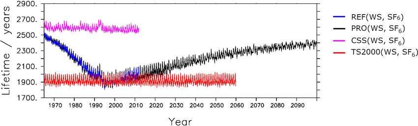
1178                                                                                S. Loeffel et al.: The impact of SF6 sinks on AoA

Table 1. Chemical reactions of SF6 . The labeling of the various reactions mirrors the style used by Reddmann et al. (2001). Reactions labeled
with † are included in the SF6 submodel.

                             Reaction no.    Reaction                           Description
                             (R1)            SF6 + hν −→ SF5 + F                Destructive
                                                                                UV photolysis
                             (R2)            † SF + e− −→ (SF− )∗               Destructive
                                                 6            6
                                             SF6 + O+ −→ SF+5 + OF
                                                                                Electron Attachment
                                             SF6 + N+       +                   and secondary Reactions
                                                    2 −→ SF5 + NF
                                             SF6 + O2 −→ SF−
                                                    −
                                                            6 + O2
                             (R3)            † SF− + hν −→ SF + e−              Photodetachment
                                                 6            6
                                                 −           +
                                             † SF + H −→ SF + HF
                             (R4)                6           5                  Destructive

                             (R5)            † (SF− )∗ + M −→ SF−               Stabilization against autode-
                                                  6             6
                                                                                tachment
                             (R6)            † (SF− )∗ −→ SF + e−               Autodetachment
                                                   6        6
                                                  −
                                             † SF + HCl −→ products
                             (R7)                 6                             Destructive
                                             SF−6 + HNO3 −→ products
                                             SF−6 + SO2 −→ products
                             (R8)            † SF− + O −→ SF + O−               Recovery reaction
                                                  6     3     6     3
                                             SF−6 + O −→ SF6 + O
                                                                 −

                                             SF−6 + NO2 −→ SF6 + NO2
                                                                      −

pute the photodetachment rate of SF−     6 , we follow Reddmann          constant climate. In the specified dynamics (SD) simulation,
et al. (2001) and use the extraterrestrial solar photon flux with        we apply Newtonian relaxation (“nudging”) towards ERA-
no attenuation of the UV-photon flux, as provided by WMO                 Interim (Dee et al., 2011) reanalysis data of potential vor-
(1986). Our simulations range from 1950 to 2011; however,                ticity, divergence, temperature, and the logarithmic surface
at least the first 10 years have to be considered as a spin-up           pressure up to 1 hPa. This assures that the meteorological sit-
period. The projection simulation runs from 1950 to 2100                 uation largely resembles the ERA-Interim data. The flexible
with the SF6 reactant species and greenhouse gases (GHGs)                structure of MESSy allows us to use the same executable
prescribed from the ESCiMo RC2-base-04 simulation (see                   for all simulations, with the differences between them re-
Jöckel et al., 2016) as monthly and zonal means. In addition             alized through changes in aforementioned namelist settings
to the reference (REF) simulation, we performed two sen-                 (see Jöckel et al., 2005). A summary of the simulations used
sitivity simulations and one specified dynamics simulation.              in this study can be found in Table 2.
The two sensitivity simulations are as follows: the CSS (con-
stant reaction partners for SF6 sinks) sensitivity simulation
differs from the REF simulation only with respect to the con-            2.4    Satellite and in situ data
stant mixing ratios of the reactant species (see above) that
influence the SF6 sinks. For that purpose, we kept the mixing            The MIPAS (Michelson Interferometer for Passive Atmo-
ratios at the level of the start of the simulation (year 1950 on         spheric Sounding) instrument on Envisat (Environmental
repeat). With this simulation, we aim to address the influence           Satellite) allowed for the retrieval of SF6 by measuring the
of the reactant species involved in the SF6 sink reactions. The          thermal emission in the mid-infrared, while orbiting the
second sensitivity simulation, referred to as TS2000, is not a           Earth sun-synchronously 14 times a day. This high-resolution
transient simulation, as is the REF simulation, but is instead           Fourier transform spectrometer measured at the atmospheric
a time slice simulation with climate conditions (GHGs; sea               limb and provided data for SF6 retrievals in full spectral res-
surface temperatures, SSTs; and SICs) of the year 2000 (cli-             olution from 2002 to 2004 and in reduced resolution from
matology of the 1995–2004 period). Furthermore, the reac-                2005 to 2012 between 6 and 40 km of altitude (Stiller et al.,
tant species for the SF6 sinks have been averaged over the               2012; Haenel et al., 2015). In this study, a newer version
1995–2004 period for the TS2000 simulation. This will al-                of the MIPAS dataset, existing as of 2019, will be shown
low us to investigate the effects of the SF6 sinks under a               (Stiller, 2021) in which new SF6 absorption cross sections
                                                                         have been used for the SF6 retrieval (Stiller et al., 2020; Har-

Atmos. Chem. Phys., 22, 1175–1193, 2022                                                       https://doi.org/10.5194/acp-22-1175-2022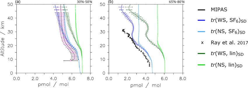
S. Loeffel et al.: The impact of SF6 sinks on AoA                                                                                              1179

Table 2. Overview of simulations undertaken in this study

                Simulation                                                       Details
                Reference (REF)                                                  Transient
                                                                                 1950–2011
                                                                                 Greenhouse gases (CO2 , CH4 , N2 O, O3 ) transiently
                                                                                 prescribed from ESCiMo RC1-base-07 simulation
                                                                                 (Jöckel et al., 2016) as monthly and zonal means
                Specified dynamics (SD)                                          Transient
                                                                                 1980–2011
                                                                                 Newtonian relaxation of dynamics towards
                                                                                 ERA-Interim reanalysis data (Dee et al., 2011)
                                                                                 up to 1 hPa
                Sensitivity simulations
                Constant reaction partners for SF6 sinks (CSS)                   Transient
                                                                                 1950–2011
                                                                                 Same conditions as the REF simulation,
                                                                                 but the year 1950 concentrations are repeated
                                                                                 throughout the model run for the SF6 reactant species
                Time slice (TS2000)                                              Time slice
                                                                                 1950–2011
                                                                                 Climate conditions (GHGs, SSTs, SICs)
                                                                                 of the year 2000
                                                                                 Climatology taken as 1995–2004
                                                                                 SF6 sinks reactant species averaged over 1995–2004
                Projection simulation
                Climate projection (PRO)                                         Transient
                                                                                 1950–2099
                                                                                 Greenhouse gases (CO2 , CH4 , N2 O, O3 ) transiently
                                                                                 prescribed from ESCiMo RC2-base-04 simulation
                                                                                 (Jöckel et al., 2016) as monthly and zonal means

              GHGs refers to greenhouse gases, SSTs refers to sea surface temperatures, and SIC refers to sea ice concentration.

rison, 2020). Except for the newer absorption cross sections                           that part of the Engel et al. (2009) AoA time series is de-
for SF6 and the consideration of a trichlorofluoromethane                              rived from CO2 measurements. In this paper, only the AoA
(CFC-11) band in the vicinity of the SF6 signature, the SF6                            data points derived from SF6 are used. Engel et al. (2017)
retrieval and conversion into AoA was done according to the                            extended the initial dataset from Engel et al. (2009) to 2016,
description by Haenel et al. (2015). In particular, the Level-                         but the AoA here is derived from CO2 measurements and is,
1b data version is still V5.                                                           thus, also excluded.
   Engel et al. (2009) collected available air samples of SF6
and CO2 from a balloon-borne cryogenic whole-air sampler
flown during 27 balloon flights, with data up to 43 km, and                            2.5     Analysis method
reanalyzed these samples in a self-consistent manner. The de-
                                                                                       The basic concepts for the calculation of mean AoA are in-
rived SF6 data cover the years from 1975 to 2005 (with a gap
                                                                                       troduced in Hall and Plumb (1994). In the case of a tracer
between 1985 and 1994) and the midlatitudes between 32
                                                                                       with a linear increasing lower boundary condition, AoA can
and 51◦ N. As AoA profiles from midlatitudes above approx-
                                                                                       be determined by the time lag between the mixing ratio at
imately 25 km or 30 hPa are constant over altitude, a mean
                                                                                       a given point in the atmosphere and the same mixing ratio
midlatitude middle-stratospheric AoA value from each pro-
                                                                                       of the reference time series. As for any realistic tracer, SF6
file was determined by averaging the vertical profile between
                                                                                       does not exhibit perfectly linear growth, for which adjust-
30 hPa and the top balloon flight height. With this procedure,
                                                                                       ments in the AoA calculation are needed. This study follows
a time series of midlatitude middle-stratospheric AoA val-
                                                                                       the calculation method employed by studies such as Engel
ues could be determined back to 1975. It is important to note
                                                                                       et al. (2009), which was introduced in Volk et al. (1997). The

https://doi.org/10.5194/acp-22-1175-2022                                                                     Atmos. Chem. Phys., 22, 1175–1193, 2022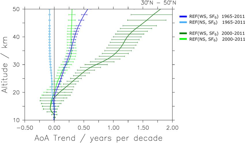
1180                                                                         S. Loeffel et al.: The impact of SF6 sinks on AoA

calculation uses a polynomial fit to the reference time se-         not perform a detailed comparison of SF6 profiles, as the ma-
ries to approximate mean AoA. However, in our study, we             jor aim is not an in-depth evaluation of the SF6 submodel
modified the parameters compared with those used in Engel           but rather a quantification of the potential effects of the SF6
et al. (2009) to ensure that (passive) SF6 -based AoA agrees        sinks on AoA and its long-term trends. However, to ensure
with the ideal AoA derived from the linear tracer, follow-          that SF6 values in the EMAC model are within the range of
ing Fritsch et al. (2020). Specifically, in our calculations, we    observational estimates, we perform selected comparisons to
used a ratio of moments of 1.0 years and a fraction of input        data from Ray et al. (2017) and MIPAS SF6 (Stiller et al.,
of 95 %. Further, we used the SF6 mixing ratio averaged over        2020, paper in preparation). Figure 1a depicts the modeled
20◦ S–20◦ N at the ground as the reference time series. Due         SF6 vertical profile climatologies in comparison with MIPAS
to the availability of data, this reference region is also used     SF6 . Figure 1b shows the modeled SF6 vertical profiles and
in Engel et al. (2009) with balloon-borne observations.             balloon-borne measurements of SF6 (Ray et al., 2017) on
   For the derivation of AoA from MIPAS SF6 observations,           a particular day. The former comparison is for zonal mean
Stiller et al. (2008, 2012) and Haenel et al. (2015) used a         SF6 averaged over 30–50◦ N and 2007–2010. These years
slightly smoothed version of the global mean of SF6 surface         have been chosen as the dataset is complete in this period.
measurements as the reference time series instead of SF6 at         The error bars represent the standard deviation of the zonal
the stratospheric entry point, which is not available from ob-      mean ensemble, which consists of the measurement noise er-
servations (see, e.g., Dlugokencky, 2005). The nonlinearity         ror of MIPAS, further random error sources from the retrieval
of the reference curve was considered by its convolution with       (e.g., temperature uncertainties), the natural variability over
an idealized age spectrum parameterized as a function of the        the longitudes of the latitude band, and the 4 years of averag-
mean age within an iterative approach. For more details, see        ing (2007–2010).
Stiller et al. (2012) and Haenel et al. (2015).                        Figure 1b shows modeled SF6 mixing ratios of the day
   In our simulations, the AoA calculations are applied to a        of the balloon flight. The balloon was launched on 5 March
total of four tracers, which can be organized into two groups.      2000 at 67◦ N in Kiruna, Sweden. To ensure that the SF6 pro-
The first assumes a strict linear growth of SF6 , producing a       file is based on air masses from within the vortex, modeled
linear reference curve, whereas the second considers a real-        SF6 values are averaged over 65–80◦ N and 0–100◦ E, which
istic growth of SF6 based on observed emissions, creating           corresponds to the area of the vortex core for the given day.
a nonlinear SF6 reference curve. Technically, in our simu-          The standard deviation of SF6 for 0–100◦ E averaged over
lations these “emissions” are realized via lower boundary           the respective latitude range is shown as error bars.
conditions, which are based on surface observations, as in             The tracers with nonlinear growth in the SD simulation
Jöckel et al. (2016). As previously mentioned, SF6 under-           show smaller tropospheric SF6 mixing ratios than the lin-
goes chemical degradation predominantly in the mesosphere.          ear tracers (Fig. 1a, b). This can be explained by the two
Consequently, the absence or presence of mesospheric sinks          different growth scenarios of SF6 and the prescribed lower
is additionally considered, resulting in a total of four tracers:   boundary conditions (see Fig. S2 in the Supplement). The
tr(WS, SF6 ), tr(NS, SF6 ), tr(WS, lin), and tr(NS, lin). The       sinks do not have a considerable effect in the troposphere;
labeling of these depends on the chemistry involved (with           hence, the effect of the SF6 sinks only becomes noticeable
sinks: “WS”; without (no) sinks: “NS”) and the growth as-           higher up. Furthermore, the effect of the SF6 depletion be-
sumed (linear: “lin”; nonlinear: “SF6 ”) and follows the pat-       comes increasingly evident with altitude. This is portrayed
tern tr(Chemistry, Growth). When referring to simulations           in the growing differences with altitude between tr(WS, lin)
with a specific tracer, the labeling will follow the notation       and tr(NS, lin) and the nonlinear equivalent. The differences
Simulation(Chemistry, Growth), and similarly we use the fol-        particularly increase for the tracers with linear emissions, as
lowing notation for AoA inferred from the tracer used in a          these exhibit higher SF6 mixing ratios and, hence, experi-
simulation: AoA(Chemistry, Growth)SIM . For example, AoA            ence greater SF6 depletion than those with nonlinear bound-
from the reference simulation based on the tracer with meso-        ary conditions. Due to the small turnaround times for air in
spheric sinks and nonlinear (SF6 -emission-based) increase is       the middle atmosphere, the tracers without sinks exhibit a
referred to as “AoA(WS, SF6 )REF ”, and AoA inferred from           very low decrease in the SF6 mixing ratios with altitude.
the linear tracer without mesospheric sinks in the reference           Figure 1a shows that the EMAC-simulated nonlinear SF6
simulation is denoted as “AoA(NS, lin)REF ”.                        is within the observed range of MIPAS SF6 . Below 30 km,
                                                                    MIPAS SF6 mixing ratios are smaller, with a near-constant
                                                                    offset of approximately 0.5 pmol mol−1 up to 20 km. Above
3   Results
                                                                    30 km, MIPAS SF6 shows larger mixing ratios than EMAC.
3.1 SF6 mixing ratios
                                                                    This means that EMAC SF6 (SD(WS, SF6 )) shows a larger
                                                                    decrease with altitude than MIPAS SF6 , suggesting that the
In order to evaluate the SF6 mixing ratios simulated by the         sinks in EMAC are too strong. Another explanation could be
EMAC model, we first analyze the four tracers in the SD sim-        overly strong vertical mixing in EMAC. However, the EMAC
ulation in comparison to observational data. This study does        SF6 lies within the MIPAS uncertainty range throughout the

Atmos. Chem. Phys., 22, 1175–1193, 2022                                              https://doi.org/10.5194/acp-22-1175-2022
S. Loeffel et al.: The impact of SF6 sinks on AoA                                                                                        1181

Figure 1. Vertical SF6 profiles for the four tracers from the SD simulation averaged over (a) 30–50◦ N (zonally averaged) for 2007–2010
and (b) 60–80◦ N, 0–100◦ E for 5 March 2000. Horizontal lines show the SF6 spread over the selected longitudes. Dark blue represents
the nonlinear tracer with sinks tr(WS, SF6 ), light blue represents the nonlinear tracer without sinks tr(NS, SF6 ), light green represents the
idealized tracer tr(NS, lin), and dark green represents the linear tracer with sinks tr(WS, lin). In panel (a), the SF6 mixing ratios obtained
from MIPAS (Stiller et al., 2020; Stiller et al., 2022) are shown in black. Black error bars depict the standard deviation of MIPAS SF6 , and
pink error bars show the systematic error of MIPAS. The systematic error is comprised of errors in the spectroscopic data and uncertainty in
the instrumental line shape, which results in a systematic error of 2 % for the lower stratosphere (10 km) and 11 % for the upper stratosphere
(60 km). See Stiller et al. (2020) for details. Black crosses in panel (b) represent the balloon-borne measurements (Ray et al., 2017) taken on
5 March 2000 at Kiruna, Sweden (67◦ N).

atmosphere. The standard deviation increase with height in                   It is based on the reaction rates (ki ) of the chemical reac-
MIPAS SF6 can be attributed to the decrease in the SF6 signal             tions (Ri ) marked in Table 1, the branching fraction  (taken
with height, which leads to an increase in the noise error of             as 0.999; see Reddmann et al., 2001), and the efficiency of
SF6 . Additionally, the natural variability in SF6 itself, as well        the SF6 -recovery reactions (η), where η is calculated as
as the evolution of SF6 over time, contribute to the increasing
                                                                               k5 (k3 + k8 ) + k6 (k3 + k4 + k7 + k8 )
standard deviation in the MIPAS SF6 profile. The increase in              η=                                           .                   (2)
the standard deviation with height can also be seen in the                         (k5 + k6 )(k3 + k4 + k7 + k8 )
EMAC SF6 profiles, particularly in the tracers tr(WS, SF6 )
and tr(WS, lin). However, it is (by far) not as large as in the              Only the realistic tracer tr(WS, SF6 ) is considered. The
MIPAS data because the simulations have no measurement                    reference simulation yields an average lifetime of 2101 years.
error and possibly show a smaller natural variability than the            Reddmann et al. (2001) carried out sensitivity experiments
observations.                                                             with this scheme, using various options for the chemical
   The balloon flight SF6 profile (Ray et al., 2014) in Fig. 1b           mechanisms. In this way, the lifetime could be varied be-
largely resembles the profile of the realistically modeled                tween 400 and 10 000 years. Our value is below the value
tracer tr(WS, SF6 ). Below 25 km, the modeled SF6 profile                 of 3200 years calculated by Ravishankara et al. (1993) but
shows a constant high bias of around 0.3 pmol mol−1 , pre-                above the values of 1278 and 850 years of the more recent
sumably due to the lower boundary conditions used. Larger                 studies by Kovács et al. (2017) and Ray et al. (2017), re-
discrepancies can be seen between 25 and 35 km altitude,                  spectively. In another new modeling study, Kouznetsov et al.
with higher mixing ratios of the modeled SF6 . As the data                (2020) presented a range of 600–2900 years. Therefore, our
presented in Fig. 1b are only for a specific day and region, the          value of around 2100 years is within, although rather at the
particular meteorological situation and location of the bal-              upper range, of the uncertainties. In contrast to the com-
loon can be crucial for the comparison.                                   parison of the model results with SF6 observations shown
                                                                          in the previous section, our lifetime value points towards
                                                                          rather weak SF6 sinks in our scheme. To assess the variabil-
3.2 SF6 lifetimes                                                         ity in the atmospheric SF6 lifetime, we show the time se-
                                                                          ries of the SF6 lifetimes for the four simulations that were
The atmospheric lifetime of SF6 can be used as an indicator               described in Sect. 2 (Fig. 2). The lifetime of the REF sim-
for the accuracy of the SF6 degradation scheme. We calculate              ulation lies at about 2500 years in 1965 and decreases by
the lifetime following Eq. (1) in Sect. 3 of Reddmann et al.              approximately 25 % to 1900 years in 2011. The lifetime of
(2001), namely                                                            the projection simulation behaves similarly and increases to
                                                                          about 2400 years by the year 2100. This shape of the lifetime
d[SF6 ]                                                                   resembles that of projected O3 (see, e.g., Eyring et al., 2007),
        = −[k1 + k2 (1 − η)][SF6 ].                             (1)      which is reflected in the ESCiMo simulations (Jöckel et al.,
  dt

https://doi.org/10.5194/acp-22-1175-2022                                                   Atmos. Chem. Phys., 22, 1175–1193, 2022
1182 S. Loeffel et al.: The impact of SF6 sinks on AoA
Figure 2. Global stratospheric and mesospheric lifetimes of SF6 calculated from the tracer with realistic lower boundary conditions and SF6
sinks (tr(WS, SF6 )). Blue represents the reference simulation (REF), black represents the projection simulation (PRO), pink represents the
constant reactant species simulation (CSS), and red represents the time slice 2000 simulation (TS2000).
2016) from which the O3 and the other SF6 reactant species values derived from SF6 in the early period (1970–1980) are
are prescribed here. However, our SF6 degradation scheme moderately affected by the sinks, with a difference of around
includes a number of simplifications, which can modify the 20 %–25 % in the polar middle stratosphere and above (i.e.,
lifetimes. For example, a constant profile is used to prescribe for mean AoA values above 5.5 years). Differences are small
the sinks through NO. This can simplify the long-term vari- (less than 10 %) for mean AoA values below 4 years. How-
ability in the SF6 lifetimes by making it overly dependent on ever, as will be discussed (see Sect. 3.5), the effect of the
the species that are transiently prescribed in the simulations. SF6 sinks increases over time, and for the later period (2000–
Apart from seasonal variations, the lifetimes of the CSS and 2010), mean AoA derived from SF6 is considerably affected
the TS2000 simulations are fairly constant, their lifetime val- by the sinks. Differences greater than 20 % can be seen in
ues lie around 2600 and 1900 years, respectively. The fact Fig. 3h) for AoA above about 3 years, and in the extratropi-
that the lifetimes of the CSS simulations are fairly constant cal lower stratosphere, differences are larger than 10 % even
implies that the long-term trends of the SF6 lifetimes can for mean AoA values of 2 years and above.
mostly be attributed to the abundance of the species involved The patterns of modeled AoA from the linear tracers are
in the SF6 degradation. Variations in stratospheric tempera- similar to those of the SF6 -emission-based tracers (compare
tures or the circulation strength seem to only play a minor Fig. 3a with Fig. 3b and Fig. 3c with Fig. 3d). However, the
role. similarities are weaker in the polar regions, especially when
the SF6 sinks are considered (Fig. 3c, d). In these regions,
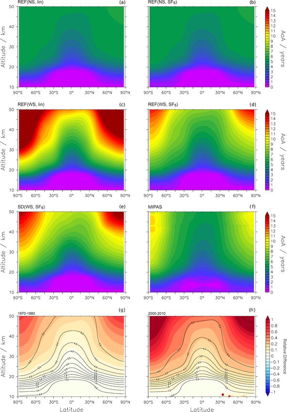
3.3 Age of air climatologies REF(WS, lin) reaches AoA values spanning 10–15 years or
more, and REF(WS, SF6 ) reaches AoA values of 9–14 years.
AoA climatologies averaged over the period from 2007 to This difference can be attributed to the greater initial growth
2010 are shown in Fig. 3: from the reference simulation for of the tracer with linear emissions than that with nonlinear
REF(NS, lin), REF(NS, SF6 ), REF(WS, lin), and REF(WS, emissions (Fig. S2). This leads to enhanced SF6 mixing ra-
SF6 ) in Fig. 3a–d, respectively; from the specified dynam- tios in the REF(WS, lin) case and, in turn, strengthens the
ics simulation (SD(WS, SF6 )) in Fig. 3e; and from MIPAS influence of SF6 sinks on AoA. This is particularly relevant
SF6 observations in Fig. 3f (Stiller, 2021). The years 2007 to in the winter months when SF6 -depleted mesospheric air is
2010 were chosen as these are the only years with complete transported downward into the polar stratosphere.
MIPAS data. AoA derived from SF6 emissions including chemical SF6
In all cases, AoA increases with increasing altitude and sinks (REF(WS, SF6 ); Fig. 3d) agrees best with MIPAS AoA
latitude. The cases considering sinks show an older apparent (Fig. 3f). Overall good agreement between EMAC and MI-
AoA than those without, especially with increasing altitude PAS AoA is found in the tropics, but there is a large high
and latitude. This apparent aging can be explained by the fact bias in the high latitudes in EMAC: between 40 and 50◦ N,
that the inclusion of mesospheric sinks results in smaller SF6 modeled AoA is up to 2 years older than MIPAS AoA in
mixing ratios. The reduced mixing ratios lead to a seemingly the stratosphere and up to 3 years older in the polar upper
older AoA as the corresponding reference value lies further stratosphere (see Fig. S5 in the Supplement). In compari-
in the past. Downwelling within the polar vortices transports son to the MIPAS observations, the SF6 sinks therefore seem
old air from the mesosphere to the stratosphere. With the to be too strong in the model, as already mentioned above.
breakdown of the polar vortex at the end of the winter season, However, in comparison with the previously published MI-
the old air is then mixed into lower latitudes. The relative ef- PAS data (Stiller et al., 2012; Haenel et al., 2015), the EMAC
fect of the sinks on AoA derived from the SF6 tracers with AoA was actually too young (i.e., the MIPAS AoA was much
nonlinear growth can be seen in Fig. 3g and h. Mean AoA
Atmos. Chem. Phys., 22, 1175–1193, 2022 https://doi.org/10.5194/acp-22-1175-2022S. Loeffel et al.: The impact of SF6 sinks on AoA 1183
Figure 3. AoA climatologies of annual means over 2007–2010. Model AoA from the reference simulation for the different tracers, tr(NS,
lin), tr(NS, SF6 ), tr(WS, lin), and tr(WS, SF6 ), is shown in panels (a)–(d), respectively, while AoA (tr(WS, SF6 )) from the specified
dynamics simulation is shown in panel (e). MIPAS AoA (Stiller, 2021) can be seen in panel (f). The relative difference between AoA(WS,
SF6 ) and AoA(NS, SF6 ) from the reference simulation for the 1970–1980 and 2000–2010 periods is shown in panels (g) and (h), respectively,
and is calculated using AoA(WS,SF 6 )−AoA(NS,SF6 ) (where 1 = 100 %). The black contours depict AoA(NS, SF )
AoA(NS,SF6 ) 6 REF for the respective time
period.
https://doi.org/10.5194/acp-22-1175-2022 Atmos. Chem. Phys., 22, 1175–1193, 20221184 S. Loeffel et al.: The impact of SF6 sinks on AoA
Figure 4. AoA time series and linear regressions calculated at 30 km averaged over 30–50◦ N. EMAC AoA from SF6 with nonlinear
emissions from the reference simulations is shown in black (REF(WS, SF6 )). AoA from the tracer with linear emissions without sinks is
shown in green (REF(NS, lin)). AoA from SF6 with nonlinear emissions with sinks in the specified dynamics simulation SD(WS, SF6 ) is
shown in pink. AoA from balloon-borne measurements (Engel et al., 2009) and AoA from MIPAS observations (Stiller, 2021) are shown in
red and dark blue, respectively.
older in the previous versions in the polar regions). The spec- that SF6 sinks have the potential to resolve the differences
troscopic data used for the SF6 retrieval in MIPAS cause a between simulated and observed climatologies of AoA and
rather large bias (that has now been corrected by improved that EMAC AoA lies within the uncertainties of MIPAS AoA
spectroscopy). The new spectroscopic data lead to a con- throughout the atmosphere. Therefore, we consider our sim-
siderably younger AoA in the middle to upper stratosphere. ulations suitable for studying the temporal evolution of AoA.
There are, however, good reasons to believe that the most
recent MIPAS data are improved compared with the previ- 3.4 Apparent age of air trends
ous ones: the spectroscopic data used are far better charac-
terized than the previous ones (Harrison, 2020), and the new In this section, we analyze the EMAC AoA trends and
AoA data from MIPAS agree significantly better with inde- compare them with observation-based AoA trends. Figure 4
pendent measurements than the previous version, in partic- shows the AoA time series and linear regressions from the
ular at higher altitudes (Stiller et al., 2020; Stiller, 2021). REF and the SD simulations as well as from MIPAS obser-
On the other hand, free-running EMAC simulations gener- vations (Stiller, 2021) and from the SF6 measurements by
ally have an overly weak Antarctic polar vortex (see Jöckel Engel et al. (2009). As the latter were collected from balloon
et al., 2016), which is, however, stronger than that of the ref- flights in the Northern Hemisphere midlatitudes at around
erence simulation. Therefore, the more stable vortex in the 30 km altitude, the EMAC and MIPAS data are also taken
SD simulation leads to enhanced isolation and aging of po- from that height and averaged over 30–50◦ N for consistency.
lar stratospheric air, especially in the Southern Hemisphere For better quantification of the trends, Table 3 provides the
during austral spring (see Fig. S4 in the Supplement for de- AoA trend values of the EMAC simulations for two periods.
tails). This could somewhat resolve the issue for the com- The trend in the entire simulation period from 1965 to 2011
parison with the previous MIPAS AoA version (see Stiller is taken for long-term trend assessment and comparison with
et al., 2012, and Haenel et al., 2015, for further details); for the measurements by Engel et al. (2009). For the compari-
the present MIPAS version, however, the discrepancies in the son with MIPAS data, the EMAC AoA trends are shown for
high altitudes and latitudes with the EMAC SD simulation the 2002–2011 period between 30 and 50◦ N, for the realis-
are even larger than with the REF simulation. The compari- tic tracer tr(WS, SF6 ). The trend calculation follows that of
son of Fig. 3e with Fig. 3f illustrates that the model cannot Haenel et al. (2015).
reproduce the tropical pipe and exhibits too much horizon- The tracers without SF6 sinks lead to negative AoA trends,
tal mixing, or overly slow upwelling. This could explain why which are consistent with the simulated acceleration of the
the model does not reproduce the constant AoA with height BDC in the course of climate change (e.g., Garcia and
in the midlatitudes. A detailed assessment of both the satel- Randel, 2008). Positive AoA trends are obtained for all
lite data and the model simulations is necessary to resolve tracers that take SF6 chemistry into account. The trend of
these discrepancies. In the model, dynamical effects like the 0.19 ± 0.01 yr per decade in the REF simulation (WS, SF6 )
strength of the polar vortex or the gravity wave parameteri- is within the limits of the uncertainties of the trend obtained
zation can play important roles in the downwelling strength. by Engel et al. (2009), who calculated an AoA trend of
Moreover, various processes of chemical SF6 removal can be 0.24 ± 0.22 yr per decade. This means that, in our simula-
revised and/or parameterized differently. Here, we showed tions, the sinks help to reconcile the modeled and the mea-
sured AoA trends over the recent decades. Note that Engel
Atmos. Chem. Phys., 22, 1175–1193, 2022 https://doi.org/10.5194/acp-22-1175-2022S. Loeffel et al.: The impact of SF6 sinks on AoA 1185
Table 3. EMAC AoA trends at 30 km averaged over 30–50◦ N. The calculation of the 2002–2011 trends is provided for the two relevant
simulations, REF(WS, SF6 ) and SD(WS, SF6 ), and follows the methods used in Haenel et al. (2015). The 2002–2011 trends are also provided
for the remaining simulations.
Simulation 1965–2011 trend (yr per decade) 2002–2011 trend (yr per decade)a
REF(WS, SF6 ) 0.19 ± 0.01 0.22 ± 0.12
REF(NS, SF6 ) −0.06 ± 0.01 −0.07 ± 0.06
REF(WS, lin) 0.70 ± 0.03 0.23 ± 0.22
REF(NS, lin) −0.07 ± 0.01 −0.06 ± 0.05
SD(WS, SF6 )b 0.39 ± 0.03 0.50 ± 0.13
CSS(WS, SF6 ) 0.11 ± 0.01 0.19 ± 0.08
TS2000(WS, SF6 )b 0.23 ± 0.02 0.07 ± 0.12
TS2000(NS, lin)b −0.00 ± 0.01 −0.21 ± 0.05
MIPASc 0.34 ± 0.13
Engel et al. (2009) d 0.24 ± 0.22
a Trend calculated following methods of Haenel et al. (2015). b Trend calculated over 1980–2011 at 30 km altitude. c MIPAS
trend calculated over 2002–2012. d Trend calculated over 1975–2005 between 32 and 51◦ N and between 24 and 35 km.
et al. (2009, 2017) also obtained a positive trend for AoA altitude and higher, which is mainly due to the larger un-
derived from CO2 measurements. certainty stemming from a smaller time period. This means
Haenel et al. (2015) calculated MIPAS AoA trends for the that the SF6 -based AoA trends with and without sinks are
period from 2002 to 2012 of 0.25 ± 0.11 yr per decade for not distinguishable from each other up to 20 and 22 km al-
30–40◦ N at 30 km and of 0.24 ± 0.11 yr per decade for 40– titude in the midlatitudes, depending on the period. Further-
50◦ N at 30 km. For the new MIPAS dataset, the AoA trend more, the uncertainty in the trend calculated from SF6 -based
is 0.34 ± 0.13 yr per decade. Note that these trends are cal- AoA with sinks increases with increasing altitude – this is
culated by applying a bias correction for the discontinuity to be expected, as the effect of the SF6 sinks increases with
between the two different observational periods of MIPAS increasing altitude. The trend in AoA(NS,SF6 )REF over the
(see Fig. 4); a description of the method can be found in von 2000–2011 period is positive at 25 km and negative over the
Clarmann et al. (2010). longer 1965–2011 period. However, it is important to note
Following the trend calculation used in Haenel et al. that the time period of about 1 decade implies that the trend is
(2015), the REF(WS, SF6 ) and SD(WS, SF6 ) time series strongly influenced by interannual variability (see, e.g., Diet-
show that EMAC AoA bears a good resemblance to that of müller et al., 2021). The strong influence of interannual vari-
the new MIPAS retrieval, with an AoA trend of 0.22 ± 0.12 ability also explains the difference in trend values in Fig. 5,
and 0.50 ± 0.13 yr per decade, respectively. Consistent with for which trends are calculated with a simple linear fit, ver-
the trend calculation of the MIPAS data, the variability due sus the value for a similar period in Table 3. The latter trends
to the QBO is considered by a respective term in the multi- were calculated using a regression model taking other vari-
variate linear analysis. However, this measure induces only ability modes into account to enable a comparison with MI-
small differences in the EMAC trend calculations (see Ta- PAS.
ble S1 in the Supplement for further details). Note also that
the rather short period of the MIPAS observations implies 3.5 Explanations of apparent age of air trends
rather large uncertainties in the trends because interannual
variability can have a large effect on the trend calculations. In this section, we will analyze the EMAC apparent AoA
This is also apparent from the highly variable trend signals trends, in particular the sign change of the trend when SF6
in the different simulations; for example, the TS2000(NS, sinks are switched on. For this, Fig. 6 shows the AoA
lin) exhibits a strongly negative trend over this period despite (WS,SF6 ) time series of the sensitivity simulations CSS and
no forced long-term trends. This is confirmed by a trend of TS2000 averaged between 30 and 50◦ N. For comparison,
−0.00 ± 0.01 yr per decade over the 1965–2011 period. AoA values from the reference simulation (REF(WS, SF6 )
As shown in Fig. 5, the strong deviation of SF6 -derived and REF(NS, lin)) are also included.
AoA trends holds almost throughout the stratosphere. Only In the CSS simulation, the mixing ratios of the reactant
below about 20 km altitude for the period from 1965 to 2011 species involved in the sink reactions of SF6 are held con-
are the effects of the SF6 sinks smaller than the trend uncer- stant. The CSS simulation with the realistic tracer (CSS(WS,
tainty. For the trend in the shorter time period of 2000–2011, SF6 )) shows an AoA trend of 0.11 ± 0.01 yr per decade over
effects from the SF6 sinks become significant at about 22 km the 1965–2011 period. This is lower than the AoA trend
in the reference simulation REF(WS, SF6 ) and means that
https://doi.org/10.5194/acp-22-1175-2022 Atmos. Chem. Phys., 22, 1175–1193, 20221186 S. Loeffel et al.: The impact of SF6 sinks on AoA Figure 5. Vertical profile of the linear trends of AoA(WS, SF6 )REF and AoA(NS, SF6 )REF over 30–50◦ N, calculated for the 1965–2011 and 2000–2011 time periods. Error bars depict the 2σ standard deviation of the trend over the respective time period, and the black vertical line denotes the zero line. Figure 6. AoA (at 10 hPa, averaged over 30–50◦ N) time series and linear regression of sensitivity experiments TS2000(WS, SF6 ), TS2000(NS, lin), and CSS(WS, SF6 ) shown in dark blue, light blue, and pink, respectively. The reference simulations REF(WS, SF6 ) and REF(NS, lin) are shown in black and green, respectively. while the changes in the SF6 -depletive substances influence trends for both tr(WS, SF6 ) and tr(NS, lin) reflect the nega- the magnitude of the positive trend, they cannot explain the tive contribution of the accelerating BDC to the trend, which positive sign of the AoA trend. can be seen in the idealized AoA trend from the REF sim- The TS2000 simulation is a time slice simulation with cli- ulation (NS, lin). Overall, neither changes in the SF6 sinks mate conditions of the year 2000. AoA of that simulation nor changes in the stratospheric circulation due to climate derived from the realistic tracer (TS2000(WS, SF6 )) shows change are responsible for the positive trend found in AoA a positive trend of 0.23 ± 0.02 yr per decade. This is even with sinks. Instead, the results indicate that the sinks them- stronger than the trend in the REF simulation (0.19 ± 0.01 yr selves can generate a positive trend. per decade). By definition, the TS2000 simulation does not For a complete discussion of the features that can be seen feature any changes in its climatic state nor in the composi- in Fig. 6, we now also describe the sudden decrease in tion of the atmosphere. This is reflected by the fact that the AoA(WS, SF6 ) shortly after 1982 seen in the REF simula- idealized tracer tr(NS, lin) does not show a trend in this sim- tion. It is also visible in the two sensitivity simulations (CSS ulation (see Table 3; TS2000(NS, lin): −0.00 ± 0.01). The and TS2000). This means that changes in the SF6 -depleting temporal increase in apparent AoA rise in the TS2000(WS, substances as well as climate change and volcanic activity (in SF6 ) simulation despite no climate changes therefore points particular the volcanic eruption of El Chichón in 1982) can to the fact that the SF6 sinks themselves lead to the positive be ruled out as possible causes of the drop. The solar cycle is trend. The difference between the TS2000 and the REF AoA not taken into account in the time slice simulation. The time Atmos. Chem. Phys., 22, 1175–1193, 2022 https://doi.org/10.5194/acp-22-1175-2022
S. Loeffel et al.: The impact of SF6 sinks on AoA 1187
series of the realistic SF6 tracer emissions show a stronger in- Eq. (3) into Eq. (4) gives us
crease in the 1980s (not shown). Fritsch et al. (2020) showed
that, due to this increase, the calculation of AoA based on Z∞
0
SF6 -like tracers is more sensitive to the chosen parameters in χ (t) = 1χoo · t e(−t /τ ) · G(t 0 )dt 0
the AoA derivation for this time. The drop in AoA that we t 0 =0
see is caused by this limitation of the derivation from SF6 - Z∞
like tracers. − 1χoo
0
t 0 e(−t /τ ) · G(t 0 )dt 0 . (5)
The increasing variability and trend in AoA in the last
2 decades, seen in the simulations with mesospheric SF6 t 0 =0
chemistry, can be attributed at first order to the SF6 depletion The expression under the first integral corresponds to the
reactions (see Fig. 6). In particular, the effect of mesospheric arrival time distribution G∗ (t 0 ) = exp(−t 0 /τ )G(t 0 ). This rep-
SF6 sinks is stronger with higher SF6 mixing ratios. Subse- resents the transit time distribution of a chemically depleted
quent downward transport of SF6 -depleted air into the vortex tracer with lifetime τ (see, e.g., Plumb et al., 1999; however,
and in-mixing thereof into lower latitudes after the vortex note that G∗ is not normalized in our definition, following
breakup results in apparent older AoA. This can explain that Engel et al., 2017). Note that τ is a measure of the lifetime
the annual variability increases over time due to the increase an air parcel experiences on its path of length t 0 and is re-
in SF6 mixing ratios. ferred to the path-integrated lifetime (not to be confused with
the local lifetime). The second integral in Eq. (5) is the first
4 Theoretical considerations and concept for sink moment of the arrival time distribution G∗ (t 0 ) (i.e., the mean
correction methods arrival time and is denoted as 0 ∗ ). Using these terms, Eq. (5)
can be expressed as
The following section focuses on the theoretical examina-
Z∞
tion of the link between SF6 sinks and positive AoA trends.
First, we will show, from a theoretical standpoint, that SF6 χ(t) = 1χoo t · G∗ (t 0 )dt 0 − 0 ∗ . (6)
sinks with constant destruction rates lead to a positive trend
t 0 =0
in AoA. Based on the theoretical considerations and on the
model data, we will then discuss the possibilities of a correc- For the tracer without sinks (here referred to as the passive
tion of AoA derived from SF6 data for the effects of the sinks. tracer χp (t)), the integral over G∗ (t 0 ) equals 1, and 0 repre-
Many observational mean AoA estimates are based on mea- sents the mean AoA. Equation 6 can then be rearranged to
surements of SF6 , and given that the relevance of the sinks
of the mean AoA estimates increases over time, a correction χp (t)
0=t− , (7)
method is required to obtain unbiased information on strato- 1χoo
spheric transport strengths.
The aforementioned link between the positive AoA trend giving the common expression to derive mean AoA from a
and mesospheric SF6 -depletive chemistry, based on Hall and linear increasing tracer.
Waugh (1998), is illustrated below and follows the mathe- In the case of a tracer with sinks, χs (t), the calculation of
matical formulations put forward by Hall and Plumb (1994) (apparent) mean AoA based on Eqs. (6) and (7) becomes
and Schoeberl et al. (2000). To allow for analytical expres-
Z∞
sions, we will only consider the case of a linearly increasing χs (t)
0̃ = t − = t − t · G∗ (t 0 )dt 0 + 0 ∗
tracer here, and we will further assume that the lifetime of 1χoo
SF6 is constant in time. We consider a tracer χ(t) experi- t 0 =0
encing relative loss e−t/τ with time-constant lifetime τ . Note Z∞
that τ is equivalent to the inverse of the loss rate. We denote = t 1 − G∗ (t 0 )dt 0 + 0 ∗ . (8)
the reference mixing ratio as χo (t) and assume a constant t 0 =0
growth rate of 1χoo :
The change of apparent mean AoA with time can then be
χo (t) = 1χoo · t. (3)
expressed as
For any location, we can then express the tracer mixing
ratio as Z∞
∂ 0̃
Z∞ = 1− G∗ (t 0 )dt 0 . (9)
0 ∂t
χ(t) = χo (t − t 0 ) · e(−t /τ ) · G(t 0 )dt 0 , (4) t 0 =0
t 0 =0 In the case of a passive tracer (i.e., a tracer without sinks),
where t 0 denotes the transit time; G(t 0 ) represents the Green’s G∗ (t 0 ) is equal to the age spectrum G(t 0 ); thus, its integral
function and is equivalent to the AoA spectrum. Inserting equals 1. Consequently, the AoA trend is zero in the absence
https://doi.org/10.5194/acp-22-1175-2022 Atmos. Chem. Phys., 22, 1175–1193, 2022You can also read