Technical note: Novel triple O2 sensor aquatic eddy covariance instrument with improved time shift correction reveals central role of ...
←
→
Page content transcription
If your browser does not render page correctly, please read the page content below
Biogeosciences, 18, 5381–5395, 2021
https://doi.org/10.5194/bg-18-5381-2021
© Author(s) 2021. This work is distributed under
the Creative Commons Attribution 4.0 License.

Technical note: Novel triple O2 sensor aquatic eddy covariance
instrument with improved time shift correction reveals central role
of microphytobenthos for carbon cycling in coral reef sands
Alireza Merikhi1 , Peter Berg2 , and Markus Huettel1
1 Department   of Earth, Ocean and Atmospheric Science, Florida State University, Tallahassee, FL 32306-4520, USA
2 Department   of Environmental Sciences, University of Virginia, Charlottesville, VA 22904-4123, USA

Correspondence: Markus Huettel (mhuettel@fsu.edu)

Received: 10 June 2021 – Discussion started: 15 June 2021
Revised: 7 September 2021 – Accepted: 8 September 2021 – Published: 4 October 2021

Abstract. The aquatic eddy covariance technique stands out         sediment–water interface to the larger wave-dominated ed-
as a powerful method for benthic O2 flux measurements in           dies of the overlying water column that still carried a positive
shelf environments because it integrates effects of naturally      flux signal, suggesting concurrent fluxes in opposite direc-
varying drivers of the flux such as current flow and light.        tions depending on eddy size and a memory effect of large
In conventional eddy covariance instruments, the time shift        eddies. The results demonstrate that the 3OEC can improve
caused by spatial separation of the measuring locations of         the precision of benthic flux measurements, including mea-
flow and O2 concentration can produce substantial flux er-         surements in environments considered challenging for the
rors that are difficult to correct. We here introduce a triple     eddy covariance technique, and thereby produce novel in-
O2 sensor eddy covariance instrument (3OEC) that by instru-        sights into the mechanisms that control flux. We consider
ment design eliminates these errors. This is achieved by posi-     the fluxes produced by this instrument for the permeable reef
tioning three O2 sensors around the flow measuring volume,         sands the most realistic achievable with present-day technol-
which allows the O2 concentration to be calculated at the          ogy.
point of the current flow measurements. The new instrument
was tested in an energetic coastal environment with highly
permeable coral reef sands colonised by microphytobenthos.
Parallel deployments of the 3OEC and a conventional eddy           1   Introduction
covariance system (2OEC) demonstrate that the new instru-
ment produces more consistent fluxes with lower error mar-         This study introduces a new eddy covariance instrument and
gin. 3OEC fluxes in general were lower than 2OEC fluxes,           demonstrates its functionality through a measuring series ad-
and the nighttime fluxes recorded by the two instruments           dressing benthic oxygen flux in a dynamic backreef area cov-
were statistically different. We attribute this to the elimina-    ered by highly permeable carbonate sands. The aquatic eddy
tion of uncertainties associated with the time shift correction.   covariance technique is a powerful technique for quantifying
The deployments at ∼ 10 m water depth revealed high day-           fluxes at the seafloor as it measures over any type of substrate
and nighttime O2 fluxes despite the relatively low organic         and integrates over a relatively large area (Berg et al., 2003;
content of the coarse sediment and overlying water. High           Lorrai et al., 2010; McGinnis et al., 2008). This non-invasive
light utilisation efficiency of the microphytobenthos and bot-     technique derives flux by averaging the turbulent vertical ad-
tom currents increasing pore water exchange facilitated the        vective transport of O2 (or other solutes) above the sediment
high benthic production and coupled respiration. 3OEC mea-         over time (Berg et al., 2003; Lorrai et al., 2010; McGinnis
surements after sunset documented a gradual transfer of neg-       et al., 2008). Since the vast majority of the recorded flux sig-
ative flux signals from the small turbulence generated at the      nals originates from the seafloor upstream of the instrument
                                                                   (termed “footprint”), the flux measurements include the ef-

Published by Copernicus Publications on behalf of the European Geosciences Union.
5382                                            A. Merikhi et al.: Novel triple O2 sensor aquatic eddy covariance instrument

fects of the natural flow and light fields, as well as the ben-      the calculated flux relative to the true flux (Berg et al., 2015;
thic sedimentary community (Berg et al., 2003; Lorrai et al.,        Reimers et al., 2016). To remove this potential source of er-
2010; McGinnis et al., 2008; Huettel et al., 2020). The eddy         ror, we designed a triple O2 sensor eddy covariance instru-
covariance method thus can produce flux data in dynamic              ment (3OEC) that eliminates the uncertainties caused by the
shelf ecosystems such as coral reefs that are strongly in-           spatial separation of flow and concentration measurements.
fluenced by flow and light (Long et al., 2013; Long, 2021;              The instrument was tested in the Florida Keys at an
Huettel et al., 2020). The technology so far has been adapted        exposed inner shelf site with carbonate sands, clear olig-
to measure temperature, salinity, oxygen, hydrogen, sulfide,         otrophic water, and substantial wave action, i.e. in an envi-
and nitrate fluxes (McGinnis et al., 2011; Johnson et al.,           ronment considered challenging for eddy covariance mea-
2011; Long et al., 2015; Crusius et al., 2008; Weck and              surements due to the low particle concentrations in the water
Lorke, 2017).                                                        (ADV measurements rely on sound reflection from particles)
   Since the fluxes are calculated from minute concentration         and the dynamic flows (causing the data misalignments ad-
changes measured at a high frequency required to account for         dressed in this study). We selected that site because carbonate
all water movements that transport the solute, it is critical that   sand beds are an integral part of reef environments and may
the flow data are accurately aligned in time with the associ-        play a central role in their carbon and nutrient cycles (Eyre
ated solute data. This presently is a potential source of error      et al., 2018; Santos et al., 2011; Cyronak et al., 2013). As
as conventional aquatic eddy covariance instruments cannot           warm water coral reefs grow in shallow, high-energy envi-
measure current velocities and solute concentrations in the          ronments, these sediments typically are dominated by highly
same location. Typically, current velocities are recorded with       permeable coarse sands (Yahel et al., 2002; Harris et al.,
an acoustic Doppler velocimeter (ADV) and solutes with               2015) colonised by microphytobenthos (Werner et al., 2008;
a fast-responding electrochemical or optical sensor (Kuwae           Jantzen et al., 2013). Owing to the rapid pore water ex-
et al., 2006; Berg et al., 2003; Reimers et al., 2012; Attard        change facilitated by the high permeability, biogeochemical
et al., 2016; Donis et al., 2016; Glud et al., 2010; McGin-          processes in the sediment surface layers can respond almost
nis et al., 2014; Lorke et al., 2013; Huettel et al., 2020). The     instantly to changes in flow, organic matter input, and light
tip of the solute sensor in these instruments is positioned at       (Huettel et al., 2014). This makes the eddy covariance tech-
a few centimetres horizontal distance from the ADV’s mea-            nique the unrivalled method for measuring interfacial fluxes
suring volume to prevent disturbances of the flow and the            in this environment, provided that potential errors associated
acoustic ADV signal. This spatial separation of flow and so-         with time shift correction in dynamic flows can be removed.
lute measurements causes a misalignment between the two                 The goals of this study therefore were to develop an eddy
measurement time series, which requires a time shift correc-         covariance instrument not affected by uncertainties caused
tion of the data. In environments with dynamic currents, this        by spatial separation of flow and solute measuring points and
misalignment changes continuously as direction and velocity          to demonstrate its functionality through measurements in a
of the turbulent flow varies. Algorithms were developed that         dynamic coral reef environment. The instrument measured
shift the O2 data in time such that they are synchronised with       O2 flux, which is considered a good proxy for benthic pro-
the velocity data (McGinnis et al., 2008; Berg et al., 2015;         duction and respiration (Berg et al., 2013; Glud, 2008). Com-
Reimers et al., 2016). A common procedure is to move a               parison with parallel measurements with a conventional eddy
short sequence (e.g. 15 min) of solute data in time relative to      covariance instrument reveals the improvements achieved by
the current flow data recorded at that time until a maximum          the new instrument design.
in flux is reached. In steady unidirectional flow, this proce-
dure largely can eliminate time shift errors, but it is difficult
to apply an effective correction in dynamic settings (Donis          2     Methods
et al., 2015; Reimers et al., 2016). Since the rapid changes in
solute concentration and vertical flow velocity are relatively       2.1    Triple O2 sensor eddy covariance instrument
small and affected by signal noise, a distinct maximum in                   (3OEC)
flux may not be found when time shifting the data, which
can result in erroneous corrections and fluxes. Furthermore,         The new 3OEC instrument utilises a data averaging approach
wave orbital motion in shelf environments produces oscillat-         to remove misalignments in time caused by the spatial sepa-
ing bottom currents that may change in magnitude and di-             ration of flow and O2 measurements and thereby eliminates
rection at the timescale of seconds, complicating a correct          potential errors caused by time shift corrections. The 3OEC
alignment of the data and producing further potential sources        measures simultaneously with three O2 fibre optodes posi-
of uncertainty in the flux calculations. In the conventional         tioned at 120◦ angular spacing in the same horizontal plane
eddy covariance instruments with one or two solute sensors,          around the centre point of the water volume where current
the cumulative effect of small errors in the time shift correc-      flow is measured by the ADV (Fig. 1). Assuming approxi-
tion thus can lead to significant under- or overestimates of         mately linear concentration gradients within the 6.4 cm dis-
the flux, which in extreme cases can reverse the direction of        tance between the O2 sensors – justifiable according to pla-

Biogeosciences, 18, 5381–5395, 2021                                                     https://doi.org/10.5194/bg-18-5381-2021

A. Merikhi et al.: Novel triple O2 sensor aquatic eddy covariance instrument                                                              5383

Figure 1. The triple O2 sensor eddy covariance instrument (3OEC). (a) The 3OEC deployed over carbonate sand at the study site in the
Florida Keys. (b) Positioning of the ADV sensor head (1) and the three O2 sensors (A, B, C). The average O2 concentration calculated
from the readings of the three O2 sensors approximates the concentration at the geometric centre of the red triangle (side lengths 6.4 cm)
defined by the three O2 sensor tips. This geometric centre is also the centre of the flow measuring volume of the ADV, marked as yellow
cylinder. (c) Vertical view of the positioning of the O2 sensors around the ADV measuring volume (yellow circle) that is located 15 cm
below the central sensor stem. The sensor tips are located at 3.0 cm horizontal distance from the edge of the ADV measuring volume. The
red triangle is the vertical view of the red triangle shown in (b). (d) Proof of the equivalence of the average of the three sensor readings and
the concentration at the centre of the equilateral triangle defined by the positions of the three optode sensor tips (red triangle in b and c).
We postulate that the concentration gradients between the sensor tips are linear (see also text). Accordingly, the half-way point of a side
of the triangle corresponds to the average concentration measured by the optodes at the two endpoints of that side. Applying the law of
sines and triangle congruence criteria (transitive property of congruence, angle bisector theorem, converse of angle bisector theorem), the
concentration at the centre point (M) of the equilateral triangle (ABC) equals the concentration at the vertex (M) of the right triangle defined
by one vertex of the equilateral triangle (C in the above example) and the midpoint ((A + C) / 2 in the above example) between that vertex
and the second vertex (A in the above example) on that line. According to the congruence criteria, this is valid for analogous, congruent
right triangles constructed on the other sides of the triangle. As these triangles are based on the average concentration of two vertices of the
equilateral triangle, it follows that the centre point concentration is equivalent to the average concentrations measured by the three sensors.
The heat map visualises the equivalence of the concentrations at the centre of the equilateral triangle calculated using this approach and the
average of the three sensor signals. Photographs: Markus Huettel.

nar optode readings of water column oxygen distributions in               circle corresponds to the average of the three sensor signals
turbulent flows (Glud et al., 2001; Larsen et al., 2011; Oguri            (Fig. 1d).
et al., 2007) – the O2 concentration at the location where the               The optodes are ultra-high-speed O2 -needle sensors (Py-
flow is measured can be calculated through averaging of the               roScience™ – OXR430-UHS; Table A1) with a response
three simultaneous sensor signals. The three optode tips, po-             time of 200–300 ms (Merikhi et al., 2018). The three optodes
sitioned at the corners of an equilateral triangle, present three         are pointing downward at a 45◦ angle, with their sensing
equidistant points on a circle with the measuring volume of               tips positioned at 3.7 cm horizontal distance from the cen-
the ADV at its centre. For linear concentration gradients be-             tre of the flow measuring volume. This placement, within
tween the three measuring points, it can be proven with the               the recommended distance of 10 Kolmogorov scale lengths
law of sines that the O2 concentration at the centre of this              from the ADV measuring volume (Lorrai et al., 2010), pre-
                                                                          vents any disturbance of the flow within that volume and

https://doi.org/10.5194/bg-18-5381-2021                                                             Biogeosciences, 18, 5381–5395, 2021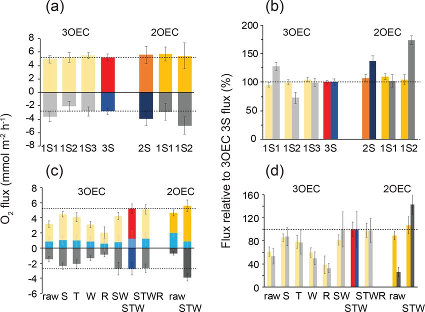
5384                                         A. Merikhi et al.: Novel triple O2 sensor aquatic eddy covariance instrument

potential interferences with the acoustic pulses of the ADV.     2.3   Data processing
The sensors are read by three FireStingO2-Mini O2 meters
(PyroScience™; Table A2). The ADV is a Nortek™ Vec-              Eddy covariance flux calculations are based on the assump-
tor acoustic Doppler velocimeter (Table A3) that measures        tion that the flux signal is transported by a bottom cur-
the 3D velocity field within a cylindrical measuring vol-        rent with steady state mean flow and O2 concentration that
ume (1.5 cm diam. × 1.5 cm, located 15 cm below the central      reaches the instrument unobstructed after passing the foot-
acoustic transducer) at a sampling rate of 32 Hz. A DataQ DI-    print area (Massman and Lee, 2002; Baldocchi, 2003; Kuwae
710-UH USB data logger (14-bit A/D conversion) records           et al., 2006; Berg et al., 2007). In coastal environments, such
simultaneously the output of O2 meters and the ADV at a          conditions rarely are met, requiring post processing of the
rate of 64 Hz to prevent aliasing. O2 meters and data log-       flux data to correct for infringements of these assumptions,
ger are contained in an underwater housing (A.G.O Envi-          as well as errors caused by technical limitations (Holtappels
ronmental Electronics) fitted with three PyroScience™ fibre      et al., 2013; Reimers et al., 2016; Huettel et al., 2020). We
feedthrough plugs for connecting the O2 sensors, as well as      applied the same routine corrections to 3OEC and 2OEC
Impulse micro inline plugs for connecting the ADV and ex-        data for compensation of design and sensor limitations, as
ternal battery (4 × lithium-ion 12 V, 50 Wh). The ADV, O2 -      well as for non-steady-state O2 concentrations in the water
meter housing, and battery pack are mounted on a stainless-      column. The unfiltered flow and O2 data records were re-
steel tripod with 1.2 m side length and 1.2 m height (Berg and   duced from 64 to 8 Hz by averaging, which reduced noise
Huettel, 2008). In addition, the frame carries a miniDOT O2      but maintained sufficient resolution to describe the entire fre-
logger (PME) and an Odyssey PAR (photosynthetically ac-          quency spectrum carrying the flux signal. For each 8 Hz time
tive radiation) logger (Dataflow Systems) for collection of      point, the average signal of the three O2 sensors of the 3OEC
temperature and O2 reference data (once per minute) and          was calculated to determine an estimate of the O2 concentra-
PAR data (once per 10 min), respectively.                        tion in the centre of the ADV measuring volume. Similarly,
                                                                 the signals of the two sensors of the 2OEC were averaged
2.2    Dual O2 sensor eddy instrument (2OEC)                     to produce mean concentrations. O2 fluxes then were calcu-
                                                                 lated based on these averages, as well as based on the sig-
An eddy covariance instrument with conventional sensor           nals of each individual sensor using the software EddyFlux
configuration (2OEC) was deployed parallel to the 3OEC to        3.2 (Peter Berg, unpublished). The software determines mean
analyse the potential flux error caused by the time shift and    O2 base concentrations for 15 min time segments through
the effectiveness of standard data corrections. The 2OEC,        Reynolds decomposition (Lorrai et al., 2010; Berg et al.,
described in detail in Huettel et al. (2020), measures si-       2009; Lee et al., 2004). Within each 15 min interval, the mean
multaneously with two O2 optodes positioned on one side          O2 concentration O2 (defined as a least-square linear fit to
of the ADV measuring volume with their measuring tips            the data) then is subtracted from each 8 Hz O2 data point to
1 cm horizontally apart. Deployments of this instrument at       arrive at the instantaneous O2 fluctuation O02 for that time
the same study site in the Florida Keys simultaneously           point. The instantaneous vertical velocity Vz0 is determined
with benthic advection chambers (Huettel and Gust, 1992;         using the same procedure. The flux at each 8 Hz time point is
Janssen et al., 2005; Huettel et al., 2020) produced eddy        calculated by multiplying the instantaneous vertical velocity
covariance fluxes (3.7 ± 0.9 mmol m−2 h−1 ) that were simi-      and associated instantaneous O2 concentration. The changes
lar to those of the chamber fluxes (3.9 ± 3.0 mmol m−2 h−1 )     in fluxes were added over time to produce cumulative flux
during daytime and of similar order of magnitude dur-            curves. For three consecutive time intervals (42 to 95 min in
ing nighttime (2OEC: −2.5 ± 1.3 mmol m−2 h−1 ; chambers:         length) with undisturbed flux during day and night, slopes
−3.4 ± 0.8 mmol m−2 h−1 ). These fluxes obtained with an         of these curves then were calculated to determine light and
independent measuring technique corroborate the magnitude        dark fluxes, respectively. In the following text, fluxes based
of the eddy covariance fluxes, but it should be noted that the   on the averaged signal of three (3OEC) or two (2OEC) O2
chambers do not account for changes in flow and organic          sensors were termed “3S-flux” and “2S-flux”, respectively.
matter supply during the incubation, which both can have         Single sensor fluxes were termed “1S-flux” and uncorrected
a significant influence on the flux. While the chambers un-      fluxes “raw” fluxes.
der relatively steady conditions and short incubation periods       Standard corrections, abbreviated in this text by single let-
can produce fluxes similar to those recorded by eddy covari-     ters, were applied to the flux data to reduce potential er-
ance instruments, discrepancies between fluxes measured by       rors caused by instrument tilt (R), wave effects (W ), time
the two techniques were observed in dynamic environments         shift (T ) – caused by spatial separation of sensors (2OEC)
(Berg et al., 2013).                                             and sensor response time – and changes in water column
                                                                 O2 storage (S) (Berg et al., 2015; McGinnis et al., 2008;
                                                                 Lorke et al., 2013; Huettel et al., 2020). Influence of poten-
                                                                 tial instrument tilt (R) on flux was tested and corrected when
                                                                 necessary through the rotation of the velocity data so that

Biogeosciences, 18, 5381–5395, 2021                                                 https://doi.org/10.5194/bg-18-5381-2021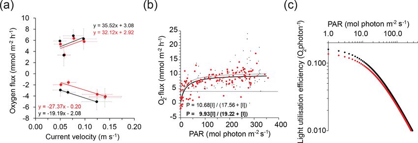
A. Merikhi et al.: Novel triple O2 sensor aquatic eddy covariance instrument                                                    5385

the mean transverse and vertical velocity were nullified (Lee        in relatively high light intensities at the seafloor reaching
et al., 2004; Lorke et al., 2013; Lorrai et al., 2010). Similarly,   392 µmol photons m−2 s−1 . On each measuring day, the in-
wave rotation (W ) was rectified by rotating the flow velocity       struments were deployed during daylight time to include the
field so that SD(Vy ) and SD(Vz ) reached a minimum (SD rep-         effect of benthic photosynthesis and were retrieved the fol-
resents 1 standard deviation) (Berg et al., 2015; Berg et al.,       lowing day for data download.
2013). Time shifts (T ) were rectified through applying time
shift corrections to the O2 data that produced the maximum
absolute fluxes (McGinnis et al., 2008; Berg et al., 2015;           3     Results
Berg et al., 2003; Reimers et al., 2016; Fan et al., 1990). Ef-
                                                                     3.1    Benthic fluxes
fects of large-scale variations in the average water column
O2 concentration (S) were compensated
                                 Rh           for through apply-     The O2 fluxes measured by the 3OEC were lower
ing an O2 storage term (JSt = 0 dC/dth, with dC/dt being             and less variable than those recorded by the 2OEC
the change in the average O2 concentration over time, calcu-         (Fig. 2a and b). Daytime 3OEC O2 fluxes averaged
lated through linear detrending of the measured O2 data over         5.2 ± 0.6(SE) mmol m−2 h−1       and     nighttime    fluxes
15 min intervals, and h = height of the measuring volume)            −2.8 ± 0.6(SE) mmol m−2 h−1 , characterising the per-
(Holtappels et al., 2013; Rheuban et al., 2014). Furthermore,        meable carbonate sand bed as a site of high carbon turnover
acceleration or deceleration of current flows can alter the O2       and net autotrophy in July 2017. Average 3OEC daytime
concentration profile and thereby temporarily modulate verti-        fluxes were 7 % lower and nighttime fluxes 38 % lower
cal flux (Holtappels et al., 2013). Our data analysis indicated      than the respective 2OEC fluxes (day 5.6 ± 0.8(SE), night
that the temporal flux variations caused by transient velocity       −3.9 ± 0.5(SE) mmol m−2 h−1 ). The difference in the night-
changes largely cancelled out over time, and a correction for        time fluxes between the two instruments was statistically
transient velocity changes was not applied.                          significant (p = 0.04685, p(x ≤ T ) = 0.02342, T = −3.268,
   All recordings in this study are referenced to eastern day-       DF = 3), while the difference in daytime fluxes was not
light time (EDT), which is 4 h behind coordinated universal          (p = 0.08077, p(x ≤ T ) = 0.9596, T = 2.5944, DF = 3).
time (UTC−4). All times in the text, graphs, and legends are         The trajectories of the cumulative fluxes were similar in
thus presented in EDT. Daytime was defined as the period             both instruments, but in the 3OEC, the additional sensor and
between sunrise and sunset. To determine the significance of         elimination of errors associated with time shift corrections
differences in fluxes measured by the two instruments, the           reduced fluctuations of the averaged signal trajectories
paired t test was utilised. Error margins are reported as ± 1        (Fig. 2c).
standard deviation unless stated otherwise.
                                                                     3.2    Time shift
2.4   Instrument deployments
                                                                     In the 3OEC, elimination of the time shift caused by spatial
The 3OEC and 2OEC were deployed at 9 ± 1 m wa-                       separation of O2 and flow measurements does not completely
ter depth on an exposed backreef carbonate platform in               remove time shift errors from the raw fluxes. The remaining
the Florida Keys (24◦ 43.5230 N, 80◦ 49.8550 W; Fig. 1a)             time shift errors are caused by the response time of the O2
on 11, 13, 15, and 16 July 2017. Prior to the deploy-                sensors (0.2–0.3 s) and temporary distortions of the O2 con-
ments, the instruments were synchronised in time. Scuba              centration field (Fig. 3).
divers placed the two instruments 10 m apart along a tran-              Within the oxygen gradient near the seafloor, vertical wa-
sect perpendicular to the main southwest–northeast flow              ter movement associated with wave orbital motion causes O2
direction. The tripods were rotated such that the x axis             oscillations at a fixed point above the sediment, i.e. at the
of the ADVs was aligned with the main current direc-                 ADV’s flow measuring point. During nighttime, O2 signal
tion, and the measuring volumes of the ADVs were ad-                 minima occur at the maxima of water parcel elevation as wa-
justed to 35 cm above the average sediment surface level.            ter originating near the O2 -consuming sediment surface is
The seafloor here is covered by highly permeable medium              moved up within the water column. Elevation z expresses
carbonate sand (median grain size: 440 µm; permeability:             the instantaneous relative elevation of a water parcel that is
3.2 × 10⁻¹¹ ± 1.2 × 10⁻¹² m2 ) with relatively low carbon            moved Rup and down at the velocity Vz and can be estimated
content (0.23 % ± 0.05 % sed. dw.) and colonised by mi-              as z = Vz dt (Berg et al., 2015). In the 4 min recording ex-
crophytobenthos (Chlorophyll a: 4.9 ± 0.1 µg g−1 sed. dw.).          ample shown in Fig. 3, nearly parallel vertical connecting
During the deployment week, water temperatures averaged              lines between the O2 concentration minima recorded by the
29.9 ± 0.3 ◦ C and salinity 35.0 ± 0.5. Bottom current veloc-        three optodes during time intervals with reduced wave activ-
ities ranged from 5 to 14 cm s−1 . Waves increased from 11           ity (e.g. 40–60, 90–120, 210–220 s) confirm that the sensor
to 15 July, when maximum wave heights of 90 cm were                  response times were similar and consistent. Bending in the
reached, and then dropped again on 16 July. The weather              connecting lines during periods with increased wave activity
was mostly sunny with some scattered clouds resulting                (reflected by larger pressure oscillations; Fig. 3e) reveals dis-

https://doi.org/10.5194/bg-18-5381-2021                                                      Biogeosciences, 18, 5381–5395, 2021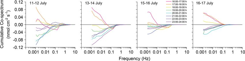
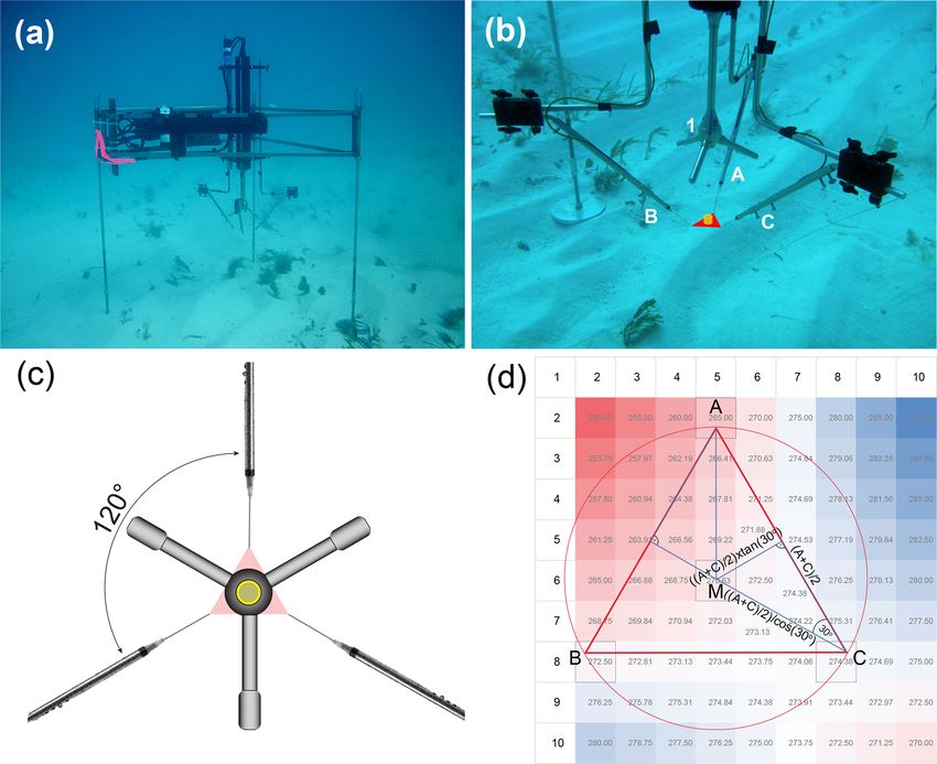
5386                                             A. Merikhi et al.: Novel triple O2 sensor aquatic eddy covariance instrument

Figure 2. Fluxes and cumulative flux trajectories recorded during the deployment week. (a) Daytime and (b) nighttime O2 fluxes measured
by the 3OEC (red circles and line) and 2OEC (black circles and line), as well as significant wave heights (light blue triangles and line) and
current flows (green diamonds and line) recorded in July 2017. Note reversed y axis scale for (b) night fluxes. Grey circle in (b) indicates
data point compromised by sensor deterioration. Error bars depict standard deviation except for the 11–16 July averages (single circles on
right side of panels), for which error bars present standard error. (c) Comparison of cumulative fluxes measured by the 3OEC (left column)
and 2OEC (right column) on 11–12, 13–14, 15–16, and 16–17 July (top to bottom) with the respective light (PAR) intensities (orange lines)
at the seafloor. Sensor 1: red; sensor 2: blue; sensor 3: green; average sensor signals: thick black lines.

tortions of the O2 concentration field at the scale of the oxy-          total time shift caused by sensor response time plus transi-
gen sensor spacing (i.e. within the triangle in Fig. 1b). Since          tory shifts produced by distortion during these 4 min aver-
the observed time shifts between elevation maxima and the                aged −0.36, −1.52, and −0.20 s for the three sensors, re-
associated O2 signal minima are positive as well as negative,            spectively, and −0.59 s for the 3S signal. To compensate for
the bending cannot be attributed to optode response charac-              sensor response time, a time shift correction was included in
teristics, implying that it is caused by distortions in the O2           the corrections (STW) used when calculating all 3S-fluxes.
concentration field. Such distortions temporarily move the               The temporary time shifts caused by transitory concentration
3S signal slightly off centre in the flow measuring volume,              field distortions largely average out over time as reflected in
producing varying time shifts between 3S signal and veloc-               the 3S variances that were 1.9 to 3.4 times smaller than the
ity data. In this example, a maximum time shift of 1.79 s                1S variances, and a correction for concentration field distor-
briefly was reached at t = 183.49 s, lasting less than 6 s. The          tion was not applied.

Biogeosciences, 18, 5381–5395, 2021                                                          https://doi.org/10.5194/bg-18-5381-2021
A. Merikhi et al.: Novel triple O2 sensor aquatic eddy covariance instrument                                                               5387

Figure 3. The 4 min interval of nighttime data recorded on 13 July (04:53:20–04:57:20) comparing the simultaneous elevation, oxygen, and
pressure readings recorded by the 3OEC. Elevation expresses the instantaneous relative elevation of a water parcel that is moved up and down
in the water column (see text). (a) Elevation (blue line) and (b–d) the associated O2 concentrations recorded by the three optodes (red, blue,
and green lines) and their (e) average (black line). Brown line in (e) depicts pressure P (scale right y axis) at the height of the ADV. The data
were smoothed by a 2.5 s running average. In the absence of a time shift, a minimum in O2 change occurs when water displacement is zero,
and points with zero O2 change therefore are connected in this graph to points with no elevation change. Since this is a nighttime recording,
O2 minima cross-correlate with elevation maxima. Vertical red lines connect elevation maxima and associated O2 minima as identified by
the OriginLab 2017 software peak-finding algorithm (analysis of 2nd derivative). Vertical grey lines do the same, but in these cases one of
the minima or maxima could not be identified by the peak-finding algorithm (manual fit). The instance of the largest temporary time shift
(−1.79 s) between elevation maximum and the corresponding 3S O2 minimum observed within this 4 min interval is indicated by the vertical
purple line. The data listed below the graph reveal how the averaging of the O2 signals reduces the variance of the O2 signal in the flow
measuring volume relative to the individual O2 signals.

3.3   Uncertainties and flux corrections                                   from the respective normalised 3S-flux and 2S-flux (Fig. 4b).
                                                                           Corrections for storage (S) and time shift (T ; in 3OEC to
                                                                           correct for response time) increased raw flux, while correc-
3OEC fluxes based on the 3S signal had lower standard er-                  tions for wave rotation (W ) and instrument tilt (R) reduced it
rors than fluxes based on individual 1S signals, i.e. standard             (Fig. 4c). Applying a combination of storage, time shift, and
error was reduced by 27 % ± 35 % (1 SD) during daytime                     wave rotation corrections (STW) led to the best agreement
and 114 % ± 158 % (1 SD) during nighttime (Fig. 4a). The                   between 1S-fluxes, as well as to the strongest enhancement
normalised daytime 1S-fluxes deviated 3 % (3OEC) and 2 %                   of the raw flux (Fig. 4c and d), as previously found in 2OEC
(2OEC) and nighttime fluxes 18 % (3OEC) and 26 % (2OEC)

https://doi.org/10.5194/bg-18-5381-2021                                                              Biogeosciences, 18, 5381–5395, 2021
5388 A. Merikhi et al.: Novel triple O2 sensor aquatic eddy covariance instrument
Figure 4. Comparison of fluxes based on single sensor signals and average signals, as well as the effects of flux corrections. Error bars
represent standard error. (a) Comparison of the daytime (yellow/orange) and nighttime (grey/dark grey) fluxes averaged over all days based on
individual sensors and sensor averages (day: red/brown, night: blue/dark blue). (b) Normalised 1S-, 2S-, and 3S-fluxes, colour code as in (a).
The 3S-flux (red/blue) was set to 100 % (all data in (a) and (b) are STW-corrected). (c) Effect of corrections on 3S and 2S daytime, nighttime,
and 24 h fluxes (light blue) averaged over all days (error bars SE). Raw: not corrected; S: storage-corrected; T : time-shift-corrected; W : wave
rotation-corrected; R: rotation-corrected. SW, STW, and STWR are combinations of the above corrections. (d) Normalised differences
between the 3OEC STW-corrected average fluxes (set to 100 %) and fluxes with no correction or different corrections recorded with the
3OEC and the 2OEC. Column colour coding in (c) and (d) as listed for (a). Dotted lines allow for the comparison of the fluxes with the
3S-fluxes. Corresponding graphs based on the individual sensor readings are included in the Supplement.
deployments conducted at the same study site (Huettel et al., Improved precision and the generally lower fluxes in the
2020). 3OEC were reflected in the community photosynthesis-
irradiance (PI) curves (Bernardi et al., 2015). The 3OEC
3.4 Effects of waves, unidirectional currents, and light predicted a slightly lower maximum gross benthic pri-
mary production (GPP) of 9.9 mmol O2 m−2 h−1 (R 2 : 0.999)
At our study site, waves were relatively high for this shal- than the 2OEC (10.7 mmol O2 m−2 h−1 , R 2 : 0.998; Fig. 5b),
low environment (wave height up to 10 % of water depth), as well as a lower light utilisation efficiency (LUE; ra-
and wave orbital motion influenced water movement and tio between GPP and PAR, 3OEC LUE 12.3 % lower than
pressure near the seafloor during the entire study (e.g. 2OEC LUE at 10 µmol photon m−2 s−1 and 7.4 % lower at
Fig. 3e). Yet, fluxes scaled with the average unidirectional 350 µmol photon m−2 s−1 ; Fig. 5c). Due to the scatter in the
bottom current velocity, which slowed during the deploy- data, these differences in GPP maxima and LUE were statis-
ment week (∼ 30 mmol m−2 h−1 flux increase or decrease tically not significant.
per metre per second flow decrease; Fig. 5a), and not with
significant wave height (R 2 < 0.04; Fig. 2a and b) that in-
creased during the study except the last day. On that last 4 Discussion
day, significant wave heights were nearly identical to those
recorded 3 d earlier (Fig. 2a and b; day 0.31 and 0.31 m 4.1 3OEC, 2OEC, and advection chamber fluxes
and night 0.27 and 0.24 m for 13–14 and 16–17 July,
respectively), but daytime fluxes decreased by 47 % and The 3OEC improves benthic flux measurements through the
sand nighttime fluxes by 58 % between these deployments. addition of the third concentration sensor, which eliminates
Light was ruled out as a cause for the decreases in the errors that can be produced by time shifts between concen-
fluxes over time because light conditions were similar be- tration and flow measurements. The averaging of the three
tween deployment days (858 ± 165 mmol photon m−2 sur- instantaneous concentration signals also reduces signal vari-
face PAR for the overlapping time period 17:00–20:00). ance and uncertainties that can arise from the disagreement
Biogeosciences, 18, 5381–5395, 2021 https://doi.org/10.5194/bg-18-5381-2021A. Merikhi et al.: Novel triple O2 sensor aquatic eddy covariance instrument 5389
Figure 5. Effect of flow and light on flux. (a) Effect of flow velocity on day- and nighttime fluxes measured with the 3OEC (red circles
and line) and 2OEC (black circles and line). The data points indicate the average fluxes calculated for light daytime and dark nighttime
periods, separated at 20:00, plotted against the average flow velocity for the respective time periods. Compromised data point from the
16 July 2OEC deployment was excluded from regression (grey circle). Error bars represent standard error. (b) Increase in daytime fluxes
with increasing light intensity at the seafloor. Black curves depict photosynthesis-irradiance curves (red circles, thick line: 3OEC; black dots,
thin line: 2OEC) calculated using Michaelis–Menten kinetics (P = Pmax [I ]/(KI + [I ]), with P being the photosynthetic rate at a given light
intensity, Pmax the maximum potential photosynthetic rate, [I ] the light intensity, and KI the half-saturation constant, i.e. the light intensity
at which the photosynthetic rate proceeds at 1/2 Pmax ). The horizontal black line indicates approximate level of daytime respiration. (c) Light
utilisation efficiency of the benthic community based on data shown in (b) (red circles: 3OEC; black circles: 2OEC).
Table 1. Comparison of 3OEC and 2OEC key characteristics. Approximate costs as of August 2021. Not included are costs for support frame
(custom made) and additional sensors (e.g. light, temperature, same for both instruments).
Factors affecting instrument choice 3OEC 2OEC
Performance during test deployments
Differences in observed magnitude of O2 fluxes
Normalised daytime flux relative to 3OEC 100 % 106 % ± 6 %
Normalised nighttime flux relative to 3OEC 100 % 151 % ± 46 %
Precision during test deployments
Normalised average standard deviation in daytime flux 18 % ± 9 % 50 % ± 35 %
Normalised average standard deviation in nighttime flux 33 % ± 11 % 51 % ± 21 %
Time required for set-up
Instrument assembly from transport boxes to deployment-ready 1–2 h 1–1.5 h
Instrument deployment programming 1h 0.5 h
Calibration 1h 0.5 h
Total time for set-up 3–4 h 2–2.5 h
Time for memory card removal and data download 0.5 h 0.5 h
Turn-around time for re-deployment 1h 0.5 h
Dimensions
Height 150 cm 150 cm
Width 120 cm 120 cm
Weight above water 40 kg 30 kg
Approximate costs
1 × vector (Nortek) USD 13 279
4 × batteries with 1 × housing (Nortek) USD 1905
1 × data logger (DataQ) USD 695
3 × (2 × 2OEC) O2 meters with underwater fibre connectors (PyroScience) USD 6498 USD 4332
3 × (2 × 2OEC) ultra-high-speed O2 optodes (PyroScience) USD 1392 USD 928
1 × electronics underwater housing for O2 meters, 300 m (AGO Env.) USD 2600
Total USD 25 969 USD 23 339
https://doi.org/10.5194/bg-18-5381-2021 Biogeosciences, 18, 5381–5395, 20215390 A. Merikhi et al.: Novel triple O2 sensor aquatic eddy covariance instrument
in two of three concentration sensor readings (Table 1). The for our four deployments indicate that during the transition
measuring approach of the aquatic eddy covariance tech- from light to dark (Fig. 6, 16:00–19:00, warm colours), tur-
nique – determining fluxes at a distance from their origin – bulence with a frequency < 0.1 Hz (larger eddies) still con-
inherently produces data with relatively large variance. This tained an upward-directed positive flux signal, while the
can raise questions regarding their reliability. The fluxes higher-frequency turbulence (smaller eddies) already carried
recorded with the 3OEC are validated by the general agree- a downward-directed negative flux signal. As the microphy-
ment of the magnitudes and trends of the 3OEC, 2OEC, tobenthos photosynthetic O2 production declined with the
and benthic advection-chamber-based fluxes (Huettel et al., decreasing light intensity at the seafloor, flux switched from
2020) all measured at the same study site, as well as benthic benthic O2 release to O2 uptake. The co-spectra suggest that
fluxes reported by Long (2021). Long’s study site with car- the ensuing negative benthic flux signal initially was trans-
bonate sands at 6 m water depth off Key Largo (Florida) was ported by the faster smaller eddies generated at the rough and
close (68.5 km distance) to ours, and the fluxes he recorded O2 -consuming sediment–water interface, while the slower
in June 2018 reached 5 mmol O2 m−2 h−1 during daytime and large eddies higher in the water column still carried the pos-
−3 mmol O2 m−2 h−1 during nighttime, similar to the fluxes itive flux signal. The co-spectra document the gradual mix-
we measured (5.2, −2.8 mmol O2 m−2 h−1 ). ing of the smaller eddies with negative flux signal into the
large eddies with positive flux signal, i.e. the negative flux
4.2 3OEC measurements in dynamic environments dip in the daytime co-spectra broadened with decreasing light
conditions, expanding from the higher to lower frequencies.
The 3OEC improves benthic flux measurements in dynamic This eddy memory effect decreased with the general de-
shelf environments. Here waves can produce artefacts in crease in bottom current velocity during our field campaign
eddy covariance flux measurements (Berg et al., 2015), as less high-frequency, small eddy turbulence is created at
which in our 3OEC measurements were reduced by the elim- the sediment–water interface at lower flow velocities (Lee
ination of errors that can be caused by the spatial separation and Cheung, 1999; Sleath, 1974). Consequently, the nega-
of concentration and flow measurements. Long (2021) pro- tive dip in the daytime co-spectra disappeared, and the co-
posed positioning the eddy covariance measurement point spectra appeared almost undisturbed in the last deployment
higher in the water column to decrease flux bias caused by (16–17 July) when bottom currents were low.
waves. Our 35 cm measuring height was identical to that
Long (2021) used for his measurements over Florida Keys’ 4.4 O2 fluxes in permeable carbonate reef sands
sands and may have contributed to further reducing potential
wave artefacts in our measurements. Our findings reveal that The O2 fluxes recorded by the 3OEC characterised the coarse
horizontal bottom currents dominated benthic flux modula- carbonate reef sands as sites of intense benthic production
tion at our site despite the significant wave action (Figs. 2a and coupled respiration. The nighttime O2 consumption rates
and b and 5a) in agreement with results of earlier studies that of the coral sand rival respiration rates measured in shallow
found an enhancing effect of current on flux in shallow shelf shelf sediments with much higher organic carbon content
environments with permeable sediment (Berg et al., 2013; (Glud, 2008; Middelburg et al., 2005; Hopkinson and Smith,
Chipman et al., 2016; McGinnis et al., 2014). Continuous 2005; Laursen and Seitzinger, 2002) and are within the
flow may be more effective than oscillating flow in driving range reported from other coral reef sands (Cyronak et al.,
advective pore water exchange in permeable sediments. In 2013; Eyre et al., 2013; Grenz et al., 2003; Rasheed et al.,
contrast to the steady pressure gradients that drive pore water 2004; Wild et al., 2005, 2004). Since the coral sands at
exchange under continuous unidirectional bottom currents, our site are low in organic carbon (< 0.3 % dw) and occur
wave orbital motion produces oscillating gradients which en- in an oligotrophic subtropical reef environment with low
hance turbulence in the pore space of the sand (Cardenas, water column chlorophyll and dissolved organic carbon con-
2008; Horton and Pokrajac, 2009; Jouybari et al., 2020). This tent (NO3 + NO2 < 0.2 µmol L−1 , NH4 < 0.5 µmol L−1 ,
turbulence and inertial losses associated with the accelera- PO4 < 0.05 µmol L−1 , Chl a < 0.2 µg L−1 , DOC <
tion and deceleration of the pore flows may lessen the effec- −1
200 µmol L ; Markus Huettel unpublished), a substan-
tiveness of the oscillating pressure gradients for driving pore tial sedimentary source of reduced compounds is required
flows and interfacial water exchange. to maintain the observed high respiration rates. Our
measurements point to benthic primary production as
4.3 The 3OEC facilitates detailed analyses this source. The compensation light intensity (intensity
at which O2 production exceeds respiration), reached at
Reduced uncertainties and higher precision achieved with ∼ 12 µmol photons m−2 s−1 , and the high light utilisation
the 3OEC facilitates more detailed analyses at higher tem- efficiency of 0.09–0.10 O2 per photon near the theoretical
poral resolution (Fig. 6). This can produce new insights in limit (0.12 O2 per photon; Brodersen et al., 2014; Attard
the processes controlling fluxes at the seafloor. Co-spectra and Glud, 2020) indicated that the microphytobenthos
time series, plotted for hourly intervals from 16:00 to 24:00 could maintain excess production under cloudy conditions,
Biogeosciences, 18, 5381–5395, 2021 https://doi.org/10.5194/bg-18-5381-2021A. Merikhi et al.: Novel triple O2 sensor aquatic eddy covariance instrument 5391
Figure 6. Change in the cumulative co-spectra for the 3S O2 flux during the deployment week. Cumulative co-spectra were calculated
for hourly intervals from 16:00 to 24:00 for the four deployment periods (0.12 nmol cm−2 s−1 corresponds to 4.3 mmol m−2 h−1 ). Colours
indicate the time periods for which the co-spectra were calculated, with red, orange, and yellow (warm colours) depicting light periods before
sunset (green). Blue and purple colours depict dark periods after sunset.
identifying the sedimentary microalgae as the source for ments as reflected in the nighttime fluxes recorded by the
the intense organic matter production and export. The 3OEC that differed significantly from those measured by the
estimated maximum production of ∼ 10 mmol m−2 h−1 2OEC. We believe that especially in dynamic settings, the
in the Florida carbonate sands (Fig. 5b) is in line with improvements in flux determinations clearly outweigh the
rates reported for reef lagoon sediments in Moorea (Pmax downsides associated with the slightly higher complexity of
6.8 ± 0.5 mmol m−2 h−1 ; Boucher et al., 1998), New Caledo- the 3OEC relative to conventional eddy covariance instru-
nia (Pmax ∼ 10 mmol m−2 h−1 ; Clavier and Garrigue, 1999), ments with one or two solute sensors. As summarised in Ta-
and the Great Barrier Reef (Pmax ∼ 11 mmol m−2 h−1 ; ble 1, the increases in set-up time and costs are modest and
Eyre et al., 2013). To put these rates into perspective, may be justified by the improvement of quality and reliability
eddy covariance flux measurements over dense Mediter- of the flux data that can be achieved with the new instrument
ranean Posidonia seagrass meadows (13 m depth, PAR (Table 1).
300–400 µmol photons m−2 s−1 ) revealed daytime O2 O2 flux is a key indicator for changes in benthic
fluxes of 6.8 ± 0.7 mmol m−2 h−1 and nighttime fluxes of metabolism and ecosystem health (Glud, 2008), emphasis-
−3.6 ± 0.4 mmol m−2 h−1 (Koopmans et al., 2020), i.e. rates ing the need for reliable flux estimates. The aquatic eddy co-
of the same magnitude as measured in the microphytoben- variance technique arguably is the best available method for
thos communities. This suggests that the benthic metabolic measuring flux at the seafloor as it does not alter activities
activity in these shallow oligotrophic environments is largely of benthic fauna and flora but integrates effects of patchiness
controlled by light. The trends of nighttime respiration and accounts for the effects flow, light, temperature, and the
that mirrored those of daytime production (Figs. 2a and b supply of electron donors and acceptors that affect the fluxes.
and 5a) indicate that at our site microphytobenthos drove The increased precision and reliability of the 3OEC data al-
the high O2 consumption rates through its respiration and low for improved modelling and ecological interpretation. In
by producing highly degradable organic matter that was many environmental measuring tasks, a basic, inexpensive
promptly recycled by the benthic heterotrophic community. instrument can produce data that are relatively close to the
Factors contributing to the high microbial activity in the “true” values, and the effort and cost for improving the qual-
carbonate sands include the high specific surface area of ity of these data typically increase exponentially with gain
the biogenic grains, their permeability to water and gases, in data accuracy and precision. The recent developments in
the organic content of the grains, their chemical buffering affordable optode technology allow a three-optode aquatic
capacity, and their light guiding characteristics (Marcelino eddy covariance instrument to be set up at modest extra cost
et al., 2013; Huettel et al., 2014; Wild et al., 2006, 2005). relative to a conventional two-optode instrument. The 3OEC
is an improved eddy covariance instrument that requires less
data post-processing and produces flux data of higher quality
5 Conclusions and reliability. It presents a hardware solution that permits
flux measurements also in dynamic shallow shelf environ-
The deployments of the 3OEC demonstrate that the new in-
ments and is an unmatched instrument to study and improve
strument can improve the precision and reliability of benthic
flux extraction methodologies. We consider the O2 fluxes
flux measurements. 3OEC fluxes in general were smaller,
produced by this instrument for the permeable reef sands
less variable, and had smaller error margins than those pro-
as some of the most realistic flux estimates achievable with
duced by the conventional 2OEC eddy covariance instrument
present-day technology.
that was deployed next to the 3OEC. The advantages of the
3OEC may be most valuable in shallow energetic environ-
https://doi.org/10.5194/bg-18-5381-2021 Biogeosciences, 18, 5381–5395, 20215392 A. Merikhi et al.: Novel triple O2 sensor aquatic eddy covariance instrument
Appendix A
Table A1. Specifications of the PyroScience™ OXR430-UHS retractable oxygen mini sensors used in this study.
Optical O2 fibre sensor type PyroScience™ OXR430-UHS
Fibre diameter 430 µm
Optimal measuring range 0–720 µmol L−1
Maximum measuring range 0–1440 µmol L−1
Detection limit 0.3 µmol L−1
Resolution at 1 % O2 0.16 µmol L−1
Resolution at 20 % O2 0.78 µmol L−1
Accuracy at 1 % O2 ± 0.31 µmol L−1
Accuracy at 20 % O2 ± 3.13 µmol L−1
Temperature range 0–50 ◦ C
Table A2. Specifications of the PyroScience™ FireStingO2 -Mini oxygen meter used in this study.
PyroScience™ FireStingO2 -Mini Single sensor module
Oxygen port One fibre-optic ST-connector
Temperature port 4-wire PT100, −30–150 ◦ C, 0.02 ◦ C resolution, ± 0.5 ◦ C accuracy
Dimensions and weight 67 mm × 25 mm × 25 mm, 70 g
Measuring principle Luminescence lifetime detection (REDFLASH)
Excitation wavelength 620 nm (orange-red)
Emission wavelength 760 nm (NIR)
Maximum sampling rate 20 Hz
Interface Serial interface (UART), ASCII communication protocol
Analogue output 0–2.5 V DC, 14-bit resolution
Power requirements Max. 70 mA at 5 V DC from USB (typ. 50 mA)
Table A3. Specifications of the NORTEK Vector acoustic Doppler velocimeter used in this study.
Sensor Range Accuracy Precision/resolution
Velocity ± 0.01, 0.1, 0.3, 1, 2, 4, 7 m s−1 ± 0.5 % ±1%
Pressure 0–20 m (shallow water version) 0.5 % (full scale) < 0.005 % of full scale
Temperature −4 to +40 ◦ C 0.1 ◦ C 0.01 ◦ C
Compass 360◦ 2◦ 0.1◦
Tilt < 30◦ 0.2◦ 0.1◦
Code and data availability. Data recorded by the 3OEC instru- Supplement. The supplement related to this article is available on-
ment 11–17 July 2017 are available at the Biological and Chem- line at: https://doi.org/10.5194/bg-18-5381-2021-supplement.
ical Oceanography Data Management Office (BCO-DMO, https:
//www.bco-dmo.org/, last access: 30 September 2021). These
archived data include current flow, pressure, and oxygen concen- Author contributions. AM deployed the 3OEC, analysed the data,
trations (https://doi.org/10.26008/1912/bco-dmo.849934.1, Huet- and wrote the first version of the manuscript. MH designed and built
tel and Berg, 2021a), reference temperature and dissolved the 3OEC instrument. MH and PB contributed to the data analysis
oxygen (https://doi.org/10.26008/1912/bco-dmo.849915.1, Huettel and the preparation of the manuscript.
and Berg, 2021b), and PAR data (https://doi.org/10.26008/1912/
bco-dmo.849979.1, Huettel and Berg, 2021c).
The EddyFlux software is available to readers upon request to
Peter Berg.
Biogeosciences, 18, 5381–5395, 2021 https://doi.org/10.5194/bg-18-5381-2021A. Merikhi et al.: Novel triple O2 sensor aquatic eddy covariance instrument 5393
Competing interests. The contact author has declared that neither Berg, P., Reimers, C. E., Rosman, J. H., Huettel, M., Delgard,
they nor their co-authors have any competing interests. M. L., Reidenbach, M. A., and Özkan-Haller, H. T.: Technical
note: Time lag correction of aquatic eddy covariance data mea-
sured in the presence of waves, Biogeosciences, 12, 6721–6735,
Disclaimer. Publisher’s note: Copernicus Publications remains https://doi.org/10.5194/bg-12-6721-2015, 2015.
neutral with regard to jurisdictional claims in published maps and Bernardi, A., Nikolaou, A., Meneghesso, A., Chachuat, B., Mo-
institutional affiliations. rosinotto, T., and Bezzo, F.: A Framework for the Dynamic
Modelling of PI Curves in Microalgae, in: 12th Process Sys-
tems Engineering (PSE) and 25th European Society of Com-
Acknowledgements. We thank the staff of the FIO Florida Keys puter Aided Process Engineering (ESCAPE), Joint Event held in
Marine Laboratory for help with instrument deployments and sam- Copenhagen, Denmark, 31 May–4 June 2015, Pt. C, edited by:
ple collection. Gernaey, K. V., Huusom, J. K., and Gani, R., Computer Aided
Chemical Engineering, 2483–2488, 2015.
Boucher, G., Clavier, J., Hily, C., and Gattuso, J. P.: Contribu-
tion of soft-bottoms to the community metabolism (primary
Financial support. The research was conducted under NOAA per-
production and calcification) of a barrier reef flat (Moorea,
mit FKNMS-2012-137-A2 and was supported by NSF grants OCE-
French Polynesia), J. Exp. Mar. Biol. Ecol., 225, 269–283,
1334117, OCE-1851290, and OCE-1061364.
https://doi.org/10.1016/s0022-0981(97)00227-x, 1998.
Brodersen, K. E., Lichtenberg, M., Ralph, P. J., Kuhl, M., and
Wangpraseurt, D.: Radiative energy budget reveals high pho-
Review statement. This paper was edited by Jack Middelburg and tosynthetic efficiency in symbiont-bearing corals, J. R. Soc.
reviewed by Conrad Pilditch and Dirk de Beer. Interface, 11, 20130997, https://doi.org/10.1098/rsif.2013.0997,
2014.
Cardenas, M. B.: Three-dimensional vortices in single pores and
their effects on transport, Geophys. Res. Lett., 35, L18402,
https://doi.org/10.1029/2008gl035343, 2008.
References Chipman, L., Berg, P., and Huettel, M.: Benthic Oxygen Fluxes
Measured by Eddy Covariance in Permeable Gulf of Mex-
Attard, K. M. and Glud, R. N.: Technical note: Estimat- ico Shallow-Water Sands, Aquat. Geochem., 22, 529–554,
ing light-use efficiency of benthic habitats using underwa- https://doi.org/10.1007/s10498-016-9305-3, 2016.
ter O2 eddy covariance, Biogeosciences, 17, 4343–4353, Clavier, J. and Garrigue, C.: Annual sediment primary production
https://doi.org/10.5194/bg-17-4343-2020, 2020. and respiration in a large coral reef lagoon (SW New Caledonia),
Attard, K. M., Hancke, K., Sejr, M. K., and Glud, R. N.: Benthic Mar. Ecol. Prog. Ser., 191, 79–89, 1999.
primary production and mineralization in a High Arctic fjord: in Crusius, J., Berg, P., Koopmans, D. J., and Erban,
situ assessments by aquatic eddy covariance, Mar. Ecol. Prog. L.: Eddy correlation measurements of submarine
Ser., 554, 35–50, https://doi.org/10.3354/meps11780, 2016. groundwater discharge, Mar. Chem., 109, 77–85,
Baldocchi, D. D.: Assessing the eddy covariance technique https://doi.org/10.1016/j.marchem.2007.12.004, 2008.
for evaluating carbon dioxide exchange rates of ecosystems: Cyronak, T., Santos, I. R., McMahon, A., and Eyre, B. D.: Carbon
past, present and future, Glob. Change Biol., 9, 479–492, cycling hysteresis in permeable carbonate sands over a diel cy-
https://doi.org/10.1046/j.1365-2486.2003.00629.x, 2003. cle: Implications for ocean acidification, Limnol. Oceanogr., 58,
Berg, P. and Huettel, M.: Monitoring the Seafloor Using the Non- 131–143, https://doi.org/10.4319/lo.2013.58.1.0131, 2013.
invasive Eddy Correlation Technique: Integrated Benthic Ex- Donis, D., Holtappels, M., Noss, C., Cathalot, C., Hancke,
change Dynamics, Oceanography, 21, 164–167, 2008. K., Polsenaere, P., Wenzhoefer, F., Lorke, A., Meysman, F.
Berg, P., Roy, H., Janssen, F., Meyer, V., Jorgensen, B. B., Huettel, J. R., Glud, R. N., and McGinnis, D. F.: An Assessment
M., and de Beer, D.: Oxygen uptake by aquatic sediments mea- of the Precision and Confidence of Aquatic Eddy Correla-
sured with a novel non-invasive eddy-correlation technique, Mar. tion Measurements, J. Atmos. Ocean. Tech., 32, 642–655,
Ecol. Prog. Ser., 261, 75–83, 2003. https://doi.org/10.1175/jtech-d-14-00089.1, 2015.
Berg, P., Roy, H., and Wiberg, P. L.: Eddy correlation flux mea- Donis, D., McGinnis, D. F., Holtappels, M., Felden, J., and Wen-
surements: The sediment surface area that contributes to the flux, zhoefer, F.: Assessing benthic oxygen fluxes in oligotrophic deep
Limnol. Oceanogr., 52, 1672–1684, 2007. sea sediments (HAUSGARTEN observatory), Deep-Sea Res.
Berg, P., Glud, R. N., Hume, A., Stahl, H., Oguri, K., Meyer, V., and Pt. I, 111, 1–10, https://doi.org/10.1016/j.dsr.2015.11.007, 2016.
Kitazato, H.: Eddy correlation measurements of oxygen uptake Eyre, B. D., Santos, I. R., and Maher, D. T.: Seasonal, daily and diel
in deep ocean sediments, Limnol. Oceanogr.-Meth., 7, 576–584, N2 effluxes in permeable carbonate sediments, Biogeosciences,
https://doi.org/10.4319/lom.2009.7.576, 2009. 10, 2601–2615, https://doi.org/10.5194/bg-10-2601-2013, 2013.
Berg, P., Long, M. H., Huettel, M., Rheuban, J. E., McGlath- Eyre, B. D., Cyronak, T., Drupp, P., De Carlo, E. H., Sachs,
ery, K. J., Howarth, R. W., Foreman, K. H., Giblin, A. J. P., and Andersson, A. J.: Coral reefs will transition to
E., and Marino, R.: Eddy correlation measurements of oxy- net dissolving before end of century, Science, 359, 908–911,
gen fluxes in permeable sediments exposed to varying cur- https://doi.org/10.1126/science.aao1118, 2018.
rent flow and light, Limnol. Oceanogr., 58, 1329–1343,
https://doi.org/10.4319/lo.2013.58.4.1329, 2013.
https://doi.org/10.5194/bg-18-5381-2021 Biogeosciences, 18, 5381–5395, 2021You can also read