Spatiotemporal and cross-scale interactions in hydroclimate variability: a case-study in France
←
→
Page content transcription
If your browser does not render page correctly, please read the page content below
Hydrol. Earth Syst. Sci., 25, 5683–5702, 2021
https://doi.org/10.5194/hess-25-5683-2021
© Author(s) 2021. This work is distributed under
the Creative Commons Attribution 4.0 License.

Spatiotemporal and cross-scale interactions in hydroclimate
variability: a case-study in France
Manuel Fossa1 , Bastien Dieppois2 , Nicolas Massei1 , Matthieu Fournier1 , Benoit Laignel1 , and Jean-Philippe Vidal3
1 Normandie Univ, UNIROUEN, UNICAEN, CNRS, M2C, 76000 Rouen, France
2 Centre
       for Agroecology, Water and Resilience (CAWR), Coventry University, Coventry, UK
3 INRAE, UR Riverly, 5 Rue de la Doua, CS 20244, 69625 Villeurbanne CEDEX, France

Correspondence: Manuel Fossa (manuel.fossa1@univ-rouen.fr)

Received: 5 February 2021 – Discussion started: 23 March 2021
Revised: 27 September 2021 – Accepted: 11 October 2021 – Published: 4 November 2021

Abstract. Understanding how water resources vary in re-            climate (precipitation and temperature) to hydrological vari-
sponse to climate at different temporal and spatial scales is      ability (discharge). Phase–amplitude interactions are indeed
crucial to inform long-term management. Climate change             absent in discharge variability, although significant phase–
impacts and induced trends may indeed be substantially             amplitude interactions are found in precipitation and temper-
modulated by low-frequency (multi-year) variations, whose          ature. This suggests that watershed characteristics cancel the
strength varies in time and space, with large consequences         negative feedback systems found in precipitation and temper-
for risk forecasting systems. In this study, we present a spa-     ature. This study allows for a multi-timescale representation
tial classification of precipitation, temperature, and discharge   of hydroclimate variability in France and provides unique in-
variability in France, based on a fuzzy clustering and wavelet     sight into the complex nonlinear dynamics of this variability
spectra of 152 near-natural watersheds between 1958 and            and its predictability.
2008. We also explore phase–phase and phase–amplitude
causal interactions between timescales of each homogeneous
region. A total of three significant timescales of variability
are found in precipitation, temperature, and discharge, i.e.,      1   Introduction
1, 2–4, and 5–8 years. The magnitude of these timescales
of variability is, however, not constant over the different re-    Hydroclimate variability represents the spatiotemporal evo-
gions. For instance, southern regions are markedly differ-         lution of hydrological (e.g., discharge and groundwater level)
ent from other regions, with much lower (5–8 years) vari-          and climate variables (e.g., precipitation and temperature)
ability and much larger (2–4 years) variability. Several tem-      which are directly impacting hydrological variability. Study-
poral changes in precipitation, temperature, and discharge         ing how hydrological variables react to climate variability
variability are identified during the 1980s and 1990s. No-         and change is a major challenge for society, in particular for
tably, in the southern regions of France, we note a decrease       water resource management and flood and drought mitiga-
in annual temperature variability in the mid 1990s. Inves-         tion planning (IPCC, 2007, 2014, 2021). However, hydro-
tigating cross-scale interactions, our study reveals causal        logical variability is expressed at multiple timescales (La-
and bi-directional relationships between higher- and lower-        bat, 2006; Schaefli et al., 2007; Massei et al., 2007, 2017),
frequency variability, which may feature interactions within       for which the driving mechanisms remain poorly character-
the coupled land–ocean–atmosphere systems. Interestingly,          ized and understood. As suggested in Blöschl et al. (2019),
however, even though time frequency patterns (occurrence           understanding the spatiotemporal scaling, i.e., how the gen-
and timing of timescales of variability) were similar between      eral dynamics driving hydrological variability change at spa-
regions, cross-scale interactions are far much complex, differ     tial and temporal scales, represents a major challenge toward
between regions, and are not systematically transferred from       improved prediction systems (Gentine et al., 2012). Under-
                                                                   standing spatiotemporal scaling required to identify regions,

Published by Copernicus Publications on behalf of the European Geosciences Union.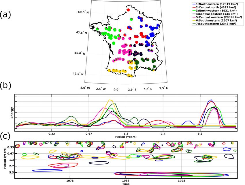
5684                                                     M. Fossa et al.: Hydroclimate variability in French spectral patterns

i.e., the maximum spatial scale in which the dynamics re-           cay et al., 2018). Cross-scale interactions are, however, very
main unchanged despite its nonlinearity, is critical (Hubert,       relevant to hydroclimate studies, in particular when search-
2001). Hydrological variability is, by definition, nonlinear        ing for climate drivers (or predictors) of hydrological signals,
(Labat, 2000; Lavers et al., 2010; McGregor, 2017) as it            as they will reveal climate timescales that are causality linked
results from complex interactions between atmospheric dy-           to each timescale of hydrological variability.
namics and catchment properties that may vary at differ-               In this study, we investigate the spatial homogeneity of hy-
ent timescales (e.g., soil characteristics, water table, karstic    droclimate variability in France across timescales. We aim at
systems, and vegetation covers; Gudmundsson et al., 2011;           identifying homogeneous regions according to specific time
Sidibe et al., 2019). Such interactions between processes           frequency patterns. From the determination of homogeneous
at different timescales, i.e., cross-scale interactions (Palus,     regions of hydroclimate variability, we will explore cross-
2014; Jajcay et al., 2018), have never been studied to further      scale interactions that may result from feedback processes
understand hydrological variability. It has also been shown         between catchment properties and hydroclimate variability.
that hydroclimate variability is inherently nonstationary, with        This study, therefore, has major implications for the com-
the time dependence of the mean and variance due to changes         prehension of hydroclimate dynamics and their interactions
in the controlling factors (e.g., Coulibaly and Burn, 2004; La-     with large-scale climate drivers and catchment properties. In
bat, 2006; Dieppois et al., 2013, 2016; Massei et al., 2017).       addition, as recently suggested in Scaife and Smith (2018),
This results in difficulties in characterizing and predicting       improved characterization of the different timescales of vari-
the hydrological variability at different spatiotemporal scales     ability and their interactions could help optimize ensemble-
(Gentine et al., 2012; Blöschl et al., 2019).                       based hydrological forecasting systems through identifying
   While different timescales have been identified in hydro-        climate ensemble members that better match the observed
logical variability (Coulibaly and Burn, 2004; Labat, 2006;         realization.
Dieppois et al., 2013, 2016; Massei et al., 2017), very lit-           The work is divided into the following sections. Data and
tle has been done to (i) explore how spatially coherent those       methods are introduced in Sect. 2. In Sect. 3, we establish
timescales are and (ii) identify regions in which the statis-       homogeneous regions for precipitation, temperature, and dis-
tical characteristics of all ranges of variability remain un-       charge variability based on their time frequency patterns and
changed. Studying 231 stream gauges throughout the world,           then explore cross-scale interactions for each region of ho-
Labat (2006) highlighted different timescales of discharge          mogeneous variability in precipitation, temperature, and dis-
variability over the different continents. At the regional scale,   charge. Finally, discussions of the main results and conclu-
Smith et al. (1998) established a clustering of 91 USA stream       sions are provided in Sect. 4.
gauges based on their global wavelet spectra, i.e., dominant
timescales, and found five homogeneous regions. Similarly,
Anctil and Coulibaly (2004) and Coulibaly and Burn (2004)
established a clustering of southern Quebec and Canadian            2     Data and methodology
streamflow, based on the timing of both the 2–3- and 3–
6-year timescales. In Europe, Gudmundsson et al. (2011)             2.1    Hydrological and climate data
identified different regions according to the magnitude of
decadal discharge variability. In France, such a clustering,        The data consist of precipitation, temperature, and discharge
based on time frequency patterns of discharge variability, and      time series located over 152 watersheds (Figs. 1, 2a and b).
its relation to climate variability (e.g., precipitation and tem-   Discharge time series were extracted from French reference
perature), has not yet been explored. In addition, all stud-        hydrometric network compiled by Giuntoli et al. (2013). This
ies mentioned above either isolated particular timescales of        network of stations identifies near-natural watersheds (i.e.,
variability or averaged the variability across timescales (e.g.,    with negligible anthropogenic modifications) with long-term,
global wavelet spectra), which is equivalent to a linearization     high-quality hydrometric data. According to Giuntoli et al.
of the system (Hubert et al., 1989). These studies thus ig-         (2013), this subset of stations does not show abrupt changes
nore potential feedback mechanisms, e.g., between soil mois-        and trends that could have resulted from anthropogenic in-
ture, precipitation, and temperature (Materia et al., 2021;         fluence. The period of 1968–2008 was chosen by Giuntoli
Ardilouze et al., 2020; Bellucci et al., 2015). In the pres-        et al. (2013) as being the best trade-off in terms of data
ence of feedback mechanisms, interactions occur over dif-           availability over the different regions. Here, this database
ferent timescales, which are also called cross-scale inter-         was further subset to 152 watersheds in order to select com-
actions (Christophe Bouton, 2017). However, while study-            plete monthly time series (i.e., without missing values) only
ing cross-scale interactions has gained increasing interest in      (Fig. 1). Precipitation and temperature data have been esti-
other fields, such as neurosciences (e.g., Onslow et al., 2014;     mated from the 8 km grid Safran surface reanalysis data set
Wang et al., 2014), cross-scale interactions are poorly under-      (Vidal et al., 2010) and have been subset to a common period
stood in climate and hydrological sciences. New strategies          (1968–2008). For this study, precipitation and temperature
have recently been developed to facilitate such studies (Jaj-       have been averaged over each watershed area (Caillouet et

Hydrol. Earth Syst. Sci., 25, 5683–5702, 2021                                        https://doi.org/10.5194/hess-25-5683-2021
M. Fossa et al.: Hydroclimate variability in French spectral patterns                                                            5685

                                                                                                                        .

Figure 1. Location of stream gauges (gray dots), corresponding watersheds (pale red; Brigode et al., 2020), hydrographic network (blue
lines; Pella et al., 2012), and orography in Safran data set (grayscale; Vidal et al., 2010)

al., 2017). Each station is thus representative of one water-        representation by projecting the time series onto a function
shed.                                                                called the mother wavelet, which quantifies the amplitude of
                                                                     the time series variability at a given timescale and time loca-
2.2     Methods                                                      tion. This mother wavelet can be translated in time to quan-
                                                                     tify the variability at precise time locations but can also be
The methodology described below (and summarized in the               scaled so that variability at different timescales can be quan-
workflow in Fig. 2) is applied to precipitation, temperature,        tified as well (Torrence and Compo, 1998; Grinsted et al.,
and discharge data sets.                                             2004). A mother wavelet at a timescale a and time location
                                                                     b is called a daughter wavelet. Daughter wavelets are calcu-
2.2.1    Continuous wavelet transforms
                                                                     lated as follows:
For each of the 152 watersheds, continuous wavelet analysis                    1

                                                                                      t −b

is used to identify at which timescales and time locations the       ψa,b = √ ψ               .                                  (1)
                                                                                a       a
amplitude of variability (i.e., local variance) is the strongest
(Fig. 2c; Torrence and Compo, 1998). Here we employ the              The left-hand side (LHS) term is the daughter wavelet of
words timescale and frequency interchangeably, though fre-           scale a and time translation b at time t. For the sake of sim-
quency implies a periodic variability, which is not a neces-         plicity, we will refer to b as the time location. The first right-
sary condition in continuous wavelet analysis. For any finite        hand side (RHS) term is the scaling of the mother wavelet ψ,
energy signal x, it is possible to obtain a time frequency           and the last one is the time translation. The projection of the

https://doi.org/10.5194/hess-25-5683-2021                                          Hydrol. Earth Syst. Sci., 25, 5683–5702, 2021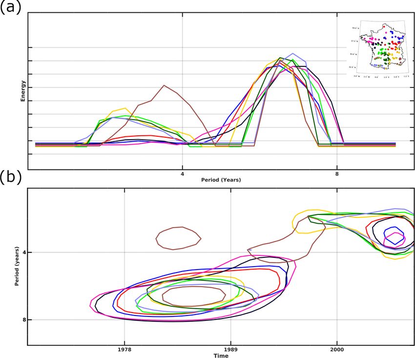
5686                                                         M. Fossa et al.: Hydroclimate variability in French spectral patterns

Figure 2. The workflow of this study is repeated for precipitation, temperature, and discharge data sets. (a) A total of 152 near-natural water-
sheds are selected. (b) Each watershed is represented by a monthly time series from 1968 to 2008, discharge is measured at a gauging station,
and precipitation and temperature are averaged over the watershed. (c) The continuous wavelet transform of each time series is computed,
representing the timescale-dependent, nonstationary variability in each watershed. (d) The similarity between all 152 continuous wavelet
transforms is computed and represented as a distance matrix. (e) Similar watersheds are grouped together into regions of homogeneous vari-
ability using a fuzzy clustering algorithm (top). For each region, the relative importance of each timescale-dependent variability is represented
with a global wavelet spectrum, and global wavelet spectra are superimposed for all regions (middle). The continuous wavelet spectra of the
regions are superimposed (bottom). For clarity, only timescale and time locations with the most significant variability are shown (colored
circles). (f) For each region, cross-timescale interactions are computed. The phase–phase interactions (top) identify any timescale’s phase
that conditions another timescale’s phase. The phase–amplitude interactions (bottom) characterize any timescale’s phase that conditions the
amplitude of another timescale.

signal onto each scale a takes the following form:                         the oscillation of signal x at scale a and centered on time
                              Z                                            location b. As it is impossible to capture the best resolution
WTψ [x](a, b) = hx, ψa,b i = x(t)ψa,b (t)dt.                      (2)      in both timescale and time location simultaneously, here we
                                                                           used a Morlet mother wavelet (of the order of 6), which offers
                                  R
                                                                           a good trade-off between the detection of scales and localiza-
The LHS term contains the wavelet coefficients, WT, i.e.,                  tion of the oscillations in time (Torrence and Compo, 1998).
how large the amplitude of variability at the timescale a and              Visualization of a continuous wavelet transform is called a
time location b is. If the mother wavelet (and, hence, the                 scalogram. Figure 2c shows a collection of scalograms, with
daughter wavelets as well) is complex, wavelet coefficients                the time location on the horizontal axis and timescale on the
are complex as well, and both the amplitude and instanta-                  vertical axis. Yellow colors show the timescales and time lo-
neous phase of the time series can be computed around time                 cations when the amplitude of the time series’ variability is
location b and timescale a. Wavelet coefficients represent the             maximum. A major advantage of continuous wavelet trans-
inner product of the signal, the daughter wavelet of scale a,              form, compared to other signal analysis methods such as the
and the time location b (center). The norm of their square                 Fourier transform, is that wavelet analysis takes nonstation-
is called the wavelet power and represents the amplitude of

Hydrol. Earth Syst. Sci., 25, 5683–5702, 2021                                                 https://doi.org/10.5194/hess-25-5683-2021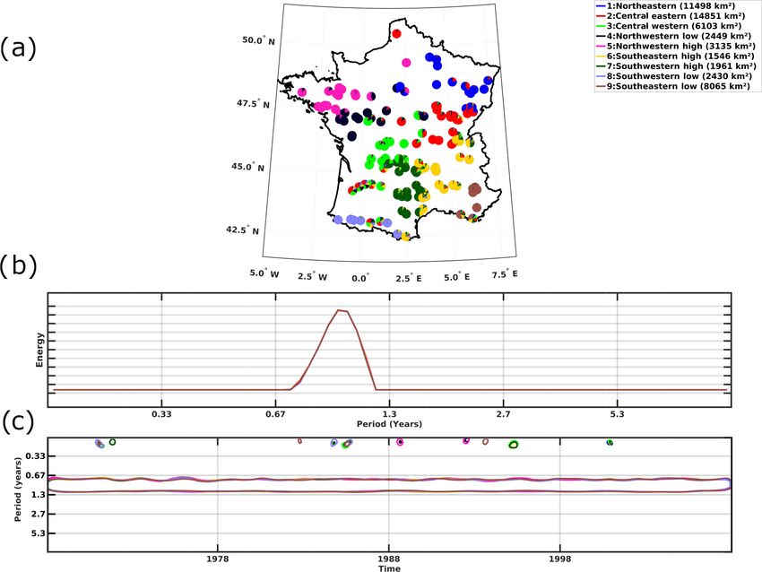
M. Fossa et al.: Hydroclimate variability in French spectral patterns                                                           5687

arity into account. Nonstationarity is the time location depen-      2.2.3   Fuzzy clustering
dence of both the mean and variance of a time series.
   Because the daughter wavelet translates and scales up,            Fuzzy clustering has then been used to cluster the different
overlaps in time and frequency can occur, and wavelet co-            watersheds based on their similarities (Fig. 2e). Fuzzy clus-
efficients can be overestimated, requiring statistical signifi-      tering is a soft clustering method (Dunn, 1973). While soft
cance tests (Torrence and Compo, 1998). This redundancy              clustering spreads membership over all clusters with vary-
may give rise to peaks in the wavelet coefficients (mean-            ing probability, hard clustering attributes each station one,
ing that high variability is detected) even in the case of a         and only one, cluster membership. Soft clustering is there-
random noise (Ge, 2007). Torrence and Compo (1998) used              fore better suited to situations when the spatial variability,
Monte Carlo simulations to assess the statistical significance       originating from different stations’ hydroclimate character-
of the continuous wavelet transform of their time series. Just       istics, is smooth. For instance, precipitation and temperature
as with any other statistical analysis, the performance of sta-      patterns are unlikely to change suddenly from one station to a
tistical tests is an open debate. It has been shown that, while      neighboring one and in turn, be markedly different from the
the significance test of Torrence and Compo (1998) may not           next neighbor (Moron et al., 2007; Hannaford et al., 2009;
unravel all significant wavelet coefficients, their false detec-     Rahiz and New, 2012). As such, several stations tend to show
tion rate is low for as long as the mother wavelet chosen            transitional or hybrid patterns and can potentially be mem-
is adapted to the time series (Ge, 2007). By using a Morlet          bers of different clusters, limiting the robustness of hard clus-
wavelet of the order of 6, we ensure that such statistical sig-      tering procedure (Liu and Graham, 2018).
nificance tests keep the false detection rate low (Ge, 2007).           Fuzzy clustering performance is determined by the ability
Because the significance test’s aim is to ensure that large          of the algorithms to recognize hybrid stations (i.e., stations
peaks are exceeding the range of variability that would oc-          incorporating multiple features from different patterns ob-
cur in a random noise, statistically significant wavelet coeffi-     served in other coherent regions), while allowing for a clear
cients are always those with large wavelet coefficients values       determination of the membership of stations with unique fea-
for any given timescale.                                             tures (Kaufman and Rousseeuw, 1990). Here, we used the
   For the reminder of this study, the terms intraseasonal, an-      FANNY algorithm (Kaufman and Rousseeuw, 1990), which
nual, and interannual refer to variations at < 1-, 1-, 2–4-, and     has been shown to be flexible and to offer the possibility to
5–8-year timescales, respectively.                                   adapt the clustering to the data with optimal performance
                                                                     (Liu and Graham, 2018). In addition, rather than setting the
2.2.2   Image Euclidean distance clustering                          number of clusters arbitrarily, we used an estimation of the
                                                                     optimum number of clusters by first computing a hard clus-
After each watershed wavelet spectrum is computed, we es-            tering method, namely consensus clustering (Monti et al.,
timate the similarity between them, i.e., how similar the vari-      2003). Thus, the number of clusters providing the best sta-
ability is, for given scales and time locations, among all           bility (i.e., the minimal changes in membership when adding
wavelet spectra (Fig. 2d). Similarities between wavelet spec-        new individuals) is considered optimal, as recommended in
tra are estimated from the entire wavelet spectrum, and not          Şenbabaoǧlu et al. (2014). The different clusters’ member-
only on statistically significant signals, to guarantee more         ships are then mapped to discuss the spatial coherence of
consistent comparison between spectra. Distances between             each hydroclimate variable.
two-dimensional data, such as wavelet spectra, are estimated
using Euclidean distance between pairwise points (pED; i.e.,         2.2.4   Cross-scale interactions
computing f2 (xi , yi ) − f1 (xi , yi )). However, such a proce-
dure has no neighborhood notion, making it impossible to             For each variable and each cluster, cross-scale interac-
account for globally similar shapes (Wang et al., 2005). To          tions are explored (Fig. 2f). Cross-scale interactions re-
avoid this issue, we used the image Euclidean distance cal-          fer to phase–phase and phase–amplitude couplings between
culation method (hereinafter IEDC) developed by Wang et              timescales of a given time series (Paluš, 2014; Scheffer-
al. (2005). The IEDC method modifies the pED equation in             Teixeira and Tort, 2016). Here, coupling means that the state
the following two ways (Wang et al., 2005): (i) the distance         (either phase or amplitude) of a signal y is dependent on the
between pixel values is computed not only pairwise but for           state of a signal x and describes causal relationship (Granger,
all indices, and (ii) a Gaussian filter, a function of the spatial   1969; Pikovsky et al., 2001), which refers to the information
distance between pixels, is applied. The Gaussian filter then        transfer from a timescale of one signal to another.
applies less weight to the computed distance between very               Figure 3 describes the necessary setting and character-
close and far apart pixels, while emphasizing on medium-             istics of cross-scale interactions. A variable (f ) measures
spaced ones (Wang et al., 2005).                                     the dynamics of a system (e.g., precipitation or temperature
                                                                     variability). This system is modeled as a coupling of two
                                                                     components (X and Y ). The components interact with each
                                                                     other in a perturbation–dampening (X and Y , respectively)

https://doi.org/10.5194/hess-25-5683-2021                                         Hydrol. Earth Syst. Sci., 25, 5683–5702, 2021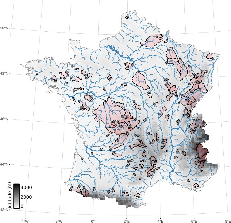
5688                                                       M. Fossa et al.: Hydroclimate variability in French spectral patterns

Figure 3. A system with directional cross-scale interactions. (a) A variable f (t) made of two components, X and Y , connected through CXY
and CY X in a perturbation–dampening scheme, so that f (t) = X(t) − Y (t). Both X and Y receive inputs φX and φY , respectively. CXX
allows X to grow first. Depending on both inputs and connections, some phase–phase or phase–amplitude interactions between X and Y can
occur. (b) An example of a phase–phase interaction, with every fourth ridge of YPP coinciding with a ridge of X, with fPP (t) = X(t)−YPP (t)
(top, middle, and bottom panels, respectively). (c) An example of a phase–amplitude interaction. X and YPA only interact when X reaches a
ridge, in which case the YPA amplitude, if lowered, yields fPA (t) (top, middle, and bottom panels, respectively; adapted from Onslow et al.,
2014).

scheme so that f (t) = X(.., t) − Y (.., t) (Fig. 3a). The in-           amplitude interaction. In Fig. 3b, YPA amplitude decreases
teractions between the components occur through the con-                 when X is at its maximum (i.e., when its phase is a ridge;
nections CXY and CY X , with a given strength (here C.. = 2),            Fig. 3c; top and middle panels). Similar to the phase–phase
and this perturbation–dampening interaction forms a nega-                interaction, fPA (t) is the difference between X(t) and YPA (t)
tive feedback (i.e., an increase in X activity triggers Y activ-         (Fig. 3c; bottom panel). Because phase and amplitude are
ity and dampens X activity, which, in turn, lowers X activity,           very dependent on inputs φX and φY , connections between
thus lowering Y activity, thus allowing X activity to increase           spatially distant physical processes are likely to give rise to
again, and so on; Fig. 3a). The connection CXX enables X to              phase–amplitude interactions (Nandi et al., 2019). In sum-
grow first before Y dampens it. This connection CXX forms                mary, there are three elements needed for cross-scale interac-
a positive feedback, i.e., increases in X activity will be more          tions between multiple, coupled processes, to arise, namely
severe as X activity is high. Both X and Y receive inputs                that (i) an oscillating forcing φX must drive X and an ad-
φX and φY from driving processes (e.g., moisture advection               ditional forcing φY on Y may also be present, (ii) X must
and convective processes; Fig. 3a). Depending on both the                have positive feedback on itself so that it grows faster than
mean and timescales of φX and φY , the strength of CXX , CXY             Y ;, and(iii) Y must show a dampening effect on X (XY or
and CY X , and X and Y may show coupled behaviors. For in-               Y X negative feedback). The presence and characteristics of
stance, in Fig. 3b, every fourth ridge of YPP (t) is synchro-            cross-scale interactions depend on the strength and frequen-
nized with a ridge of X(t) (Fig. 3b; top and middle panels),             cies of φX , φY , intrinsic frequencies of X, Y , and coupling
thus forming a phase–phase interaction. The direction of the             strengths CXY , CY X , CXX , and CY Y (Fig. 3). Thus, the detec-
interactions depends on the inputs (φX , φY ) and the connec-            tion of cross-scale interactions in time series is an indication
tions (CXX , CXY , and CY X ). fPP (t) is the difference between         of the presence of all those characteristics in the hydrocli-
X(t) and YPP (Fig. 3b; bottom panel). Because the interac-               mate system, e.g., precipitation–land processes, which helps
tion between X and Y depends on both inputs and connec-                  in investigating potential processes at play.
tions, interactions may lead to a cross-scale relationship only             The balance between X and Y determines if the feedback
for certain values of X or Y (Fig. 3c). Thus, depending on               is either positive or negative (Peters et al., 2007).
the phase of either X or Y , the amplitude of the driven com-               Note that cross-scale interactions can occur from large-
ponent may increase/decrease when the cross-scale interac-               scale to small-scale processes and vice-versa. For instance,
tion takes place and return to normal when it is out of phase            atmospheric circulation at seasonal timescales influences in-
compared to the driving component. This describes a phase–

Hydrol. Earth Syst. Sci., 25, 5683–5702, 2021                                              https://doi.org/10.5194/hess-25-5683-2021

M. Fossa et al.: Hydroclimate variability in French spectral patterns                                                        5689

terannual and decadal timescales, which, in turn, influences       3.1     Precipitation
seasonal variations (Hannachi et al., 2017).
   Following Palus (2014) and Jajcay et al. (2018), we             3.1.1    Time frequency patterns
chose the conditional mutual information (CMI) surrogates
method, combined with wavelet transforms. First, using a           The following seven regions with homogeneous time fre-
Morlet mother wavelet, the instantaneous phase and am-             quency patterns are identified (Fig. 4a): northwestern
plitude at time t and scale s of the signal are obtained.          (green), northeastern (blue), central north (red), central west-
Next, the conditional mutual information, I (φx (t); φy (t +       ern (pink), central eastern (black), southwestern (yellow),
τ ) − φy (t)|φy (t)), for the phase, and I (φx (t); Ay (t +        and southeastern (dark green). Figure 4a shows that all wa-
τ )|Ay (t)), Ay (t −η)), Ay (t −2η)), for the amplitude, is com-   tersheds converge toward singular clusters, meaning that all
puted. In the case of phase–phase relationships, the CMI           regions are highly coherent (i.e., pie charts in Fig. 4a show
measures how much the present phase of x contains informa-         one dominant color).
tion about the future phase of y, knowing the present value           In all regions, precipitation is varying at different
of y. Phase–phase interactions can be uni- or bi-directional.      timescales, ranging from intraseasonal to interannual scales
It is possible for a single timescale to drive another, which,     (i.e., 2–8 years; Fig. 4b). Southwestern and southeastern re-
in turn, drives back the original one, describing feedback         gions are dominated by annual (1 year) variability, while
interactions. For phase–amplitude relationships, CMI mea-          their interannual variability (2–8 years) is low and the reverse
sures how much the present phase of x contains information         for other regions. In addition, statistically significant areas
of the future amplitude of y, knowing the present and past         in continuous wavelet spectra show that those timescales
values of y. The statistical significance of the CMI measure       of variability are nonstationary (Fig. 4c), with temporal
is assessed using 5000 phase-randomized surrogates having          changes in terms of amplitude discriminating the different
the same Fourier spectrum and mean and standard devia-             regions. For instance, southwestern regions are character-
tion as the original time series, as seen in Ebisuzaki (1997).     ized by quasi-continuous significant annual variability until
Palus (2014) has shown that this number of surrogates is           the late 1980s, while other watersheds show sparsely signif-
ideal for statistical significance in the context of hydrocli-     icant annual variability (Fig. 4c). Similarly, although there
mate time series. The computational cost is, however, high,        is significant interannual variability in all watersheds from
with approximately 1 week of computing for a time series of        the late 1980s, during this period, southwestern and south-
50 years on a 32 core Xeon computer. The present compu-            eastern regions do not show significant interannual variations
tations were done on the Myria cluster, hosted by the Centre       (Fig. 4c). After removing the ≤ 1-year timescales (i.e., the
Régional Informatique et d’Applications Numérique de Nor-          seasonal cycle) focusing on interannual timescales, signifi-
mandie (http://www.criann.fr; last access: 7 January 2021).        cant variability at 2- (southwestern) and 5-year (southwest-
                                                                   ern and southeastern) timescales emerge for the southern re-
                                                                   gions. The largest variations (i.e., colored circles) occur over
3   Spatiotemporal clustering of hydrological variability          shorter periods of time than in other regions (Fig. 5b).
                                                                      In summary, different regions with coherent precipita-
The wavelet transform corresponding to each watershed’s
                                                                   tion variability are identified and are characterized by three
monthly time series have been computed, and all 152 water-
                                                                   timescales of variability, i.e., intraseasonal, annual, and in-
sheds’ wavelet transforms have been checked for similarities
                                                                   terannual. The amplitude of those timescales of variabil-
using IEDC fuzzy clustering to identify and characterize ho-
                                                                   ity, however, differs in time and over the French territory.
mogeneous regions of hydroclimate variability over France.
                                                                   Mediterranean regions (southwestern and southeastern) have
Once the homogeneous regions had been identified, an av-
                                                                   comparatively weaker interannual variability as compared to
erage time series for each region was computed. The global
                                                                   annual timescales. The differences between regions are both
wavelet spectrum of this time series quantified the total vari-
                                                                   dependent on the local expression of the climate forcing and
ance expressed at each timescale, while its wavelet spectrum
                                                                   watershed characteristics. Because those physical processes
characterized how this variance is distributed in the time (lo-
                                                                   are interacting, studying cross-scale interactions in precipi-
cation) and frequency (scale) domains. In addition, so as to
                                                                   tation brings more insight on the dynamics behind the spec-
focus on interannual timescales, we computed the wavelet
                                                                   tral characteristics of each region (Boé, 2013; Materia et al.,
spectrum of the time series filtered at the annual time step.
                                                                   2021; Bellucci et al., 2015; Ardilouze et al., 2020).
Cross-scale interactions were then investigated for each ho-
mogeneous region.
                                                                   3.1.2    Cross-scale interactions

                                                                   Figure 6 shows cross-scale interactions for each cluster of
                                                                   precipitation variability (see Fig. 4).
                                                                     Northeastern, southeastern, north-central, northwestern,
                                                                   and central-eastern regions all show the phase of a 5–8-

https://doi.org/10.5194/hess-25-5683-2021                                        Hydrol. Earth Syst. Sci., 25, 5683–5702, 2021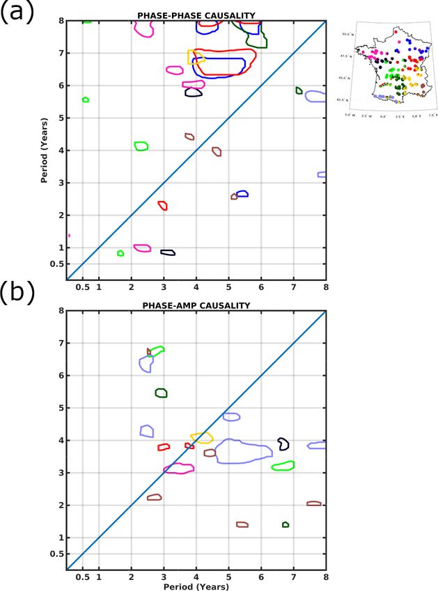
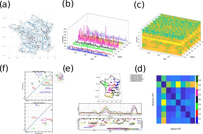
5690                                                        M. Fossa et al.: Hydroclimate variability in French spectral patterns

Figure 4. Clustering of precipitation time frequency variability in France. (a) Classification map of the watersheds. Pie chart slices show the
three highest probability memberships. Pie charts denote fuzzy clustering memberships. (b) Global wavelet spectra of homogeneous regions.
(c) Wavelet spectra of homogeneous regions. For clarity, only timescales and time locations that are 95 % statistically significant and with
the largest variability are shown (colored circles).

year variability driving the variability of smaller timescales            very weak over the southwestern regions and absent in the
(Fig. 6a; blue, dark green, red, green, and black; lower                  central-western regions.
half of the graph). This cross-scale interaction is, however,                Phase–amplitude interactions are presented in Fig. 6b.
more pronounced in the northeastern and southeastern re-                  The lower half of the graph, which refers to the lower fre-
gions (Fig. 6a). Similarly, eastern regions exclusively show              quency driving the higher-frequency variability, shows 5–8-
5–8 to 2–4-year interactions, while other regions show the                to 2–4-year interactions for the western and north-central re-
self-interacting 5–8-year variability (Fig. 6a). The upper half           gions (Fig. 6b; pink, yellow, green, and red). The central-
of the graph, which refers to the higher frequency driv-                  eastern regions are also showing the lower-frequency vari-
ing the lower-frequency variability, is populated by north-               ability driving the higher-frequency variability but between
central, southeastern, northwestern, and northeastern regions             8- and 6-year variability (Fig. 6b). Notably, the northwest-
(Fig. 6a; red, dark green, green and blue). The southeastern              ern region is the only one with cross-scale interactions driv-
region shows cascade phase–phase interactions, (i.e., from                ing the annual cycle (Fig. 6a; green). In the upper half of
2–3 and 5–4 to 6–5 years; Fig. 6a, dark green). In addition,              the graph, which refers to higher frequency driving lower-
both southeastern and northwestern regions show mirror in-                frequency variability, we only find north-central and north-
teractions with their lower-half counterparts, e.g., 5–6 to 4–            eastern regions showing 2–4- to 4- and 3–4- to 7–8-year
5 years (Fig. 6a; dark green and green mirror patches about               phase–amplitude interactions (Fig. 6b; blue and red). Note
the diagonal). We also note that phase–phase interactions are             that north-central, northeastern, and central-eastern regions

Hydrol. Earth Syst. Sci., 25, 5683–5702, 2021                                               https://doi.org/10.5194/hess-25-5683-2021
M. Fossa et al.: Hydroclimate variability in French spectral patterns 5691
Figure 5. Interannual precipitation time frequency variability in France. (a) Global wavelet spectra of homogeneous regions. (b) Wavelet
spectra of homogeneous regions. For clarity, only timescales and time locations that are 95 % statistically significant and with the largest
variability are shown (colored circles).
show phase–amplitude and phase–phase interactions at very to converge toward specific timescales, notably 2–4 and 5–
similar timescales (Fig. 6a and b; red, blue, and black), while 8 years, which were linked to ocean–atmosphere variability,
timescales of phase–amplitude and phase–phase interactions such as the North Atlantic Oscillation, in previous hydrocli-
do not match in central-western, northwestern, and south- mate studies over France (Feliks et al., 2011; Fritier et al.,
western regions (Fig. 6a and b; pink, green, and yellow). Re- 2012; Dieppois et al., 2016; Massei et al., 2017). In addition,
gions to the east, thus, appear to have both phase–phase and the presence of mirror interactions also indicate strong bidi-
phase–amplitude interactions at the same timescales, while rectional negative feedback.
western regions are more characterized by phase–amplitude
interactions. 3.2 Temperature
The precipitation cross-scale interactions can be of dif-
ferent forms, namely phase–phase, phase–amplitude, uni- or 3.2.1 Time frequency patterns
bi-directional, and from lower to higher timescales and vice
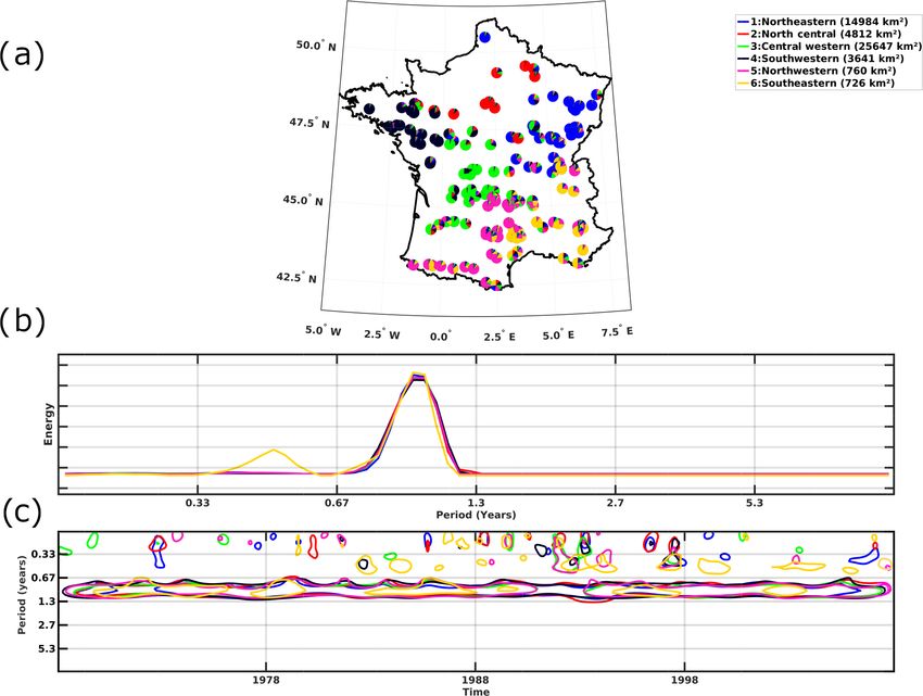
versa. The presence of cross-scale interactions seems to be In temperature, the following nine regions with homoge-
tied to specific spatial locations, suggesting different internal neous time frequency patterns are identified (Fig. 7a): north-
dynamics over the different regions of homogeneous precip- western high (pink), northwestern low (black), northeastern
itation variability. Interestingly, cross-scale interactions tend (blue), central eastern (red), central western (green), south-
eastern high (yellow), southeastern low (brown), southwest-
https://doi.org/10.5194/hess-25-5683-2021 Hydrol. Earth Syst. Sci., 25, 5683–5702, 2021
5692                                                           M. Fossa et al.: Hydroclimate variability in French spectral patterns

                                                                           1980s and 1990s in the southwestern low region, other re-
                                                                           gions show significant 2–4-year variability from the 2000s
                                                                           only (brown; Fig. 8b).

                                                                           3.2.2   Cross-scale interactions

                                                                           Figure 9 shows cross-scale interactions for each cluster of
                                                                           temperature variability identified in Fig. 8a.
                                                                              For temperature, phase–phase interactions are mostly con-
                                                                           centrated in the upper half of the graph, which refers to
                                                                           higher frequency modulating lower frequency (Fig. 9a). No-
                                                                           tably, a 2–6- to 6–8-year phase–phase interaction appears
                                                                           more pronounced over northern regions (Fig. 9a; blue, red,
                                                                           pink, and black). The central-western region shows similar
                                                                           phase–phase interactions, but at 1–3- to 4–6-year timescales
                                                                           (Fig. 9a; green). In the lower half of the graph, which refers
                                                                           to lower frequency modulating higher frequency, interactions
                                                                           are found at very similar timescales, but at slightly higher
                                                                           frequency, for all regions (e.g., 2–5- to 1–4-year variabil-
                                                                           ity; Fig. 9a). Temperature in the southwestern low region,
                                                                           however, show slightly different characteristics with phase–
                                                                           phase interactions between lower and higher frequency oc-
                                                                           curring between 7–8- and 3–4- and 7–8- to 3–4-year vari-
                                                                           ability (Fig. 9a; purple).
                                                                              Temperature phase–amplitude interactions are mostly act-
Figure 6. Precipitation cross-scale interactions (95 % significance        ing on the 3–4-year timescale for all regions (Fig. 9b). In par-
level). The driving timescale is on the horizontal axis and the driven
                                                                           ticular, in temperature, more pronounced phase–amplitude
on the vertical axis (i.e., the timescale where the x phase has a causal
                                                                           interactions are found over the southwestern low region
relationship with the phase/amplitude of the driven timescale y).
The lower (upper) half of the graph, below (above) the diagonal,           (Fig. 9b; purple), which is consistent with previous stud-
shows timescales acting on smaller (larger) timescales. (a) Phase–         ies on phase–amplitude interactions in European temperature
phase causality. (b) Phase–amplitude causality.                            (Palus, 2014; Jajcay et al., 2016). Over southwestern regions,
                                                                           temperature, however, shows both 3–8- and 3–4- and 2–4-
                                                                           and 4–7-year phase–amplitude interactions (Fig. 9b; brown
                                                                           and purple). Furthermore, it should be noted that temperature
ern high (dark green), and southwestern low (purple). Fuzzy                variability interactions occur between very similar timescales
clustering shows that watersheds typically converge toward                 over a number of regions (Fig. 9b; pink, red, yellow, and pur-
singular clusters, defining highly coherent regions (Fig. 7a).             ple). According to Palus (2014), interactions between very
This is, however, not true for the central-western region,                 similar timescales, or the same timescales, can only occur if,
which is characterized by a mix of spectral characteristic                 at least, two processes are present.
defining other regions (see the red, green, black, yellow, and                As for precipitation, in temperature, phase–phase and
purple pie charts; Fig. 7a).                                               phase–amplitude cross-scale interactions are region depen-
   Using monthly data, temperature is primarily varying on                 dent and can be uni- or bi-lateral. However, in tempera-
an annual timescale, with very similar amplitudes for all re-              ture, most phase–phase interactions occur from higher- to
gions (Fig. 7b and c). Since the dominant annual variabil-                 lower-frequency variability, while phase–amplitude interac-
ity masks the other timescales, we use the annual time step                tions tend to occur from lower- to higher-frequency variabil-
to study interannual variability (Fig. 8a and b). Focusing on              ity. Similarly, while timescales of variability that are involved
this interannual variability, significant temperature variations           for phase–phase and phase–amplitude interactions are very
indeed emerge at 2–4- and 5–8-year timescales and show                     similar in precipitation, they differ largely in temperature
different timings and amplitudes over the different regions                (Fig. 9b). This suggests that, in temperature, the processes
(Fig. 8a and b). All regions show 5–8-year variability, but,               driving phase–phase and phase–amplitude cross-scale inter-
compared to northern regions, southern regions show signif-                actions are different. It also suggests that the processes driv-
icantly stronger variations on 2–4-year timescale (Fig. 8a).               ing cross-scale interactions are different in temperature and
Similarly, while stronger 2–4-year variability occurs in the               in precipitation.

Hydrol. Earth Syst. Sci., 25, 5683–5702, 2021                                               https://doi.org/10.5194/hess-25-5683-2021
M. Fossa et al.: Hydroclimate variability in French spectral patterns 5693
Figure 7. Clustering of temperature time frequency variability in France. (a) Classification map of the watersheds. Pie chart slices show the
three highest probability memberships. (b) Global wavelet spectra of regions. (c) Wavelet spectra of homogeneous regions. For clarity, only
timescales and time locations that are 95 % statistically significant and with the largest variability are shown (colored circles).
3.3 Discharge Using monthly data, discharge is mainly varying on an-
nual timescales, as determined through the global wavelet
3.3.1 Time frequency patterns spectra (Fig. 10b). In addition, unlike other regions, south-
eastern watersheds show significant intraseasonal variability
The following six regions with homogeneous time frequency (Fig. 10b). Continuous wavelet spectra show that both annual
patterns are identified in discharge (Fig. 10a): northwestern and intraseasonal variability can be nonstationary, with tem-
(black), northeastern (blue), north central (red), central west- poral changes in terms of amplitude discriminating the differ-
ern (green), southeastern (yellow) and southwestern (pink). ent homogeneous regions of discharge variability (Fig. 10c).
However, several watersheds, especially in the south, show For instance, annual variability is only significant for spe-
memberships in multiple regions, suggesting lower spatial cific periods in the southeastern watersheds, while other re-
coherence in discharge than in precipitation and temperature. gions show quasi-continuous significant annual variability
Lower spatial coherence, however, could mostly be explained (Fig. 10c). Similarly, in the southeastern region, intrasea-
by (i) mixing of solid and liquid precipitation in driving dis- sonal discharge variability sparsely appears significant from
charge variability in the Alps and (ii) the local heterogeneity the 1980s, while they are absent in other regions (Fig. 10b).
of precipitation due to convective dynamics in the Pyrenees After removing the seasonality, and focusing on interan-
(Gottardi et al., 2008; Büntgen et al., 2008; Hermida et al., nual variability, northeastern watersheds stand out as having
2015). Nevertheless, the number of significant homogeneous continuous significant interannual variability throughout the
regions is lower in discharge than in precipitation and tem- time series, with 4–5- and 5–8-year variability before and
perature, and northern regions are particularly coherent. after the 1990s, respectively (Fig. 11b). Southeastern and
https://doi.org/10.5194/hess-25-5683-2021 Hydrol. Earth Syst. Sci., 25, 5683–5702, 20215694 M. Fossa et al.: Hydroclimate variability in French spectral patterns
Figure 8. Interannual temperature time frequency variability in France. (a) Global wavelet spectra of homogeneous regions. (b) Wavelet
spectra of homogeneous regions. For clarity, only timescales and time locations that are 95 % statistically significant and with the largest
variability are shown (colored circles).
southwestern regions also stand out, as they show 2–4-year 3.3.2 Cross-scale interactions
variability in the mid-1970s and 2000s (Fig. 11b; yellow and
pink). In addition, southeastern regions do not show signifi-
cant variability in discharge at timescales greater than 4 years An important question concerning discharge cross-scale in-
(Fig. 11a and b). teractions is whether interactions found in either precipita-
Different coherent regions are thus identified for discharge tion or temperature are also present in discharge. Phase–
variability. In addition, these homogeneous regions corre- phase interactions that were found in precipitation are also
spond well with regions identified in precipitation and tem- identified in discharge, in particular over the northeastern,
perature variability. As in precipitation and temperature, southeastern, and northwestern regions (blue, yellow, and
those regions seem strongly impacted constrained tempera- black; Figs. 6a and 12a). Phase–phase interactions that were
ture, and southern regions, which may appear more complex identified in temperature are much less evident (Figs. 9a and
in term of climate and its link to land surface processes, ap- 12a). It should also be noted that many small patches, de-
pear much less spatially coherent in discharge. scribing phase–phase interactions in precipitation and tem-
perature, are systematically not transferred to discharge vari-
ability (Figs. 6a, 9a, 12a). Instead, discharge variability
seems to exclusively preserve large patches of phase–phase
interactions (Figs. 6a, 9a, 12a), suggesting that catchment
Hydrol. Earth Syst. Sci., 25, 5683–5702, 2021 https://doi.org/10.5194/hess-25-5683-2021M. Fossa et al.: Hydroclimate variability in French spectral patterns 5695
thus smooths out and flattens phase–amplitude interactions
(Schuite et al., 2019).
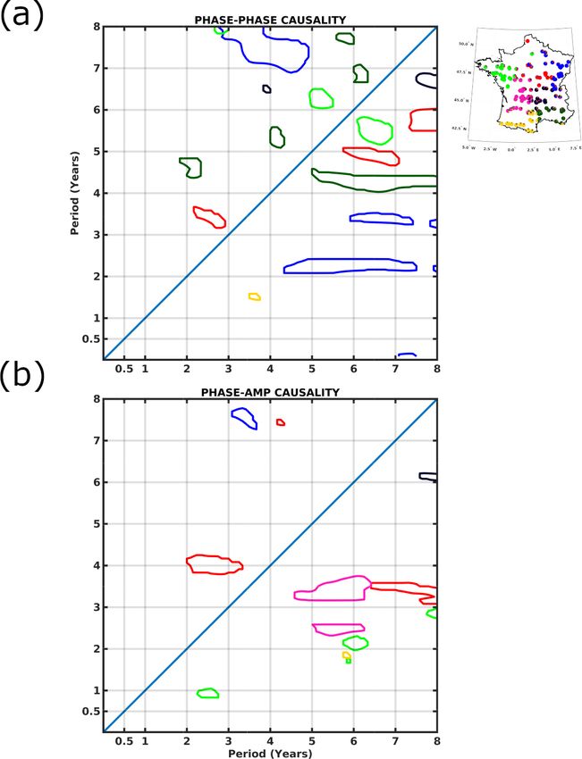
Cross-scale interactions are only of phase–phase nature in
discharge. All phase–phase interactions in discharge seem to
be primarily related to precipitation, even though the strong
correlations between rainfall and temperature makes it diffi-
cult to detect. However, differences between regions of ho-
mogeneous discharge variability are very similar to those de-
tected in precipitation. Further work is, however, needed to
understand why phase–amplitude cross-interactions are ab-
sent in discharge variability. Catchment properties appear to
involve positive rather than negative feedback, thus resulting
in a loss in phase–amplitude interactions.
4 Discussions and conclusions
4.1 Spatial variability of homogeneous hydroclimate
variability in France
As recommended by Blöschl et al. (2019), characterizing the
different scales of spatial and temporal variability, as well as
their interactions, remains one of the most important chal-
lenges in hydrology. In this study, we unraveled homoge-
neous regions of hydroclimate variability in France, account-
ing for nonstationarity and nonlinearity, bringing additional
information over previous, regime-based, classifications in
France or elsewhere (Champeaux and Tamburini, 1996;
Figure 9. Temperature cross-scale interactions (95 % significance
Bower and Hannah, 2002; Sauquet et al., 2008; Snelder et
level). The driving timescale is on the horizontal axis and the driven
on the vertical axis (i.e., the timescale x phase has a causal relation-
al., 2009; Joly et al., 2010; Gudmundsson et al., 2011). This
ship with the phase/amplitude of the driven timescale y). Lower (up- was achieved through a clustering analysis based on time fre-
per) half of the graph, below (above) the diagonal, shows timescales quency patterns of precipitation, temperature, and discharge
acting on smaller (larger) timescales. (a) Phase–phase causality. variability over 152 watersheds. We then studied the spa-
(b) Phase–amplitude causality. tiotemporal characteristics of each homogeneous region, in-
cluding characteristic timescales of hydroclimate variability
(i.e., precipitation, temperature, and discharge) and cross-
properties are modulating the climatic signals (i.e., precip- scale interactions.
itation and temperature). Such filtering of climate signals Our study reveals different coherent regions of precipita-
is even more pronounced in certain regions, such as the tion, temperature and discharge variability. Yet, some wa-
north central, where phase–phase interactions are absent in tersheds are characterized by a mix of spectral characteris-
discharge (Fig. 12a) but were identified in precipitation and tics from surrounding regions or regions with the same to-
temperature (Figs. 6a and 9a). pographic characteristics. Those coherent regions are homo-
More importantly, there is no phase–amplitude interaction geneously distributed over France in precipitation and dis-
in discharge (Fig. 12b). This points out that watershed prop- charge but show larger discrepancies in term of spatial ex-
erties modulate the interacting processes in precipitation and tension in temperature. According to previous clustering of
temperature. Because our data set is mostly composed of low hydroclimate variability over France, northern regions are
groundwater support, those modulations are unlikely to result more homogeneous than what was found here (Champeaux
from the water table, especially as phase–phase interactions and Tamburini, 1996; Sauquet et al., 2008; Snelder et al.,
are inherited from precipitation. In addition, further analy- 2009; Joly et al., 2010) and show lower spatial coherence.
sis at the Paris Austerlitz gauging station, which includes In particular, here, we demonstrate that both the amplitude
very large groundwater support, reveals the same absence of and timings of the different timescales of hydroclimate vari-
phase–amplitude interaction in discharge (not shown; Flipo ability differentiate the regions, highlighting the need for ac-
et al., 2020). Possible explanations include the frequency par- counting for nonstationary behavior in global to regional hy-
titioning of watershed compartments or integration process droclimate study. Overall, hydroclimate variability displays
along the river network breaks any spatial connection and intraseasonal (< 1 year), annual (1 year), and interannual
https://doi.org/10.5194/hess-25-5683-2021 Hydrol. Earth Syst. Sci., 25, 5683–5702, 20215696 M. Fossa et al.: Hydroclimate variability in French spectral patterns
Figure 10. Clustering of discharge time frequency variability in France. (a) Classification map of the watersheds. Pie chart slices show the
three highest probability memberships. (b) Global wavelet spectra of homogeneous regions. (c) Wavelet spectra of homogeneous regions. For
clarity, only timescales and time locations that are 95 % statistically significant and with the largest variability are shown (colored circles).
(2–4 and 5–8 years) timescales. Our results, which were fo- sue using observational data. Nevertheless, we can use the
cused on the French territory, are therefore consistent with mandatory conditions for cross-scale interactions to discuss
timescales of variability identified over the world’s major the processes that are potentially at play (Fig. 3). In pre-
rivers (Labat, 2006). cipitation, cross-scale interactions involve lower-frequency
The timescales identified in this study have been shown to timescales driving higher-frequency timescales. North At-
be important in climate processes, such as the North Atlantic lantic climate variability encompasses various processes,
Oscillation or the Gulf Stream front (Massei et al., 2007; Fe- such as North Atlantic Oscillation or sea surface tempera-
liks et al., 2010; O’Reilly et al., 2017). Their interactions ture anomalies, that drive climate variability (Feliks et al.,
with watershed characteristics likely leads to their local ex- 2010; O’Reilly et al., 2016). Thus, moisture advection from
pression with local processes, which play an important role the North Atlantic area could potentially act as a posi-
in feedback mechanisms dampening or enhancing how the tive feedback forcing. Moisture advection has indeed been
climate variability is expressed at the local scale (Haslinger shown to impact western Europe precipitation, especially in
et al., 2021; Materia et al., 2021; Bellucci et al., 2015). wintertime (Sun et al., 2020; O’Reilly et al., 2017). Zonal
moisture advection is only forcing precipitation variabil-
4.2 Cross-scale interactions ity when the region is not affected by blocking weather
regimes (Haslinger et al., 2019, 2021). Furthermore, vege-
Feedback mechanisms can occur between any physical pro- tation, temperature and soil moisture, which are themselves
cesses of the hydroclimate system, and identifying or at- interacting with each other, can act as a dampening forc-
tributing the nature of these processes is an intractable is-
Hydrol. Earth Syst. Sci., 25, 5683–5702, 2021 https://doi.org/10.5194/hess-25-5683-2021M. Fossa et al.: Hydroclimate variability in French spectral patterns 5697 Figure 11. Interannual discharge time frequency variability in France. (a) Global wavelet spectra of homogeneous regions. (b) Wavelet spectra of homogeneous regions. For clarity, only timescales and time locations that are 95 % statistically significant and with the largest variability are shown (colored circles). ing, thus dampening the precipitation. The precipitation– the authors used two climate models to simulate soil moisture temperature, precipitation–soil moisture and precipitation– sensitivity to precipitation forcing and note that this variabil- vegetation feedback have indeed been shown to reach a neg- ity is much larger in century-long reanalysis, such as NOAA’s ative sign, depending on prior state of the soil (Liu et al., 20CR. For other regions, interannual negative soil moisture 2006; Berg et al., 2015; Liu et al., 2006). However, the sign feedback was found by Boé (2013), while Sejas et al. (2014) of temperature–soil moisture–vegetation feedback on pre- found negative ocean–land temperature differences in precip- cipitation has been shown to be spatially dependent at the itation feedback. Similar results were found in Bellucci et al. global scale. For instance, while temperature and soil mois- (2015), where interactions between compartments of the at- ture have large effects in western Europe, vegetation feed- mospheric circulation at intraseasonal timescale were found back is stronger and mostly of a positive sign in northern to produce significant interannual variations. Europe (Woodward et al., 1998; Liu et al., 2006; Yang et al., Interannual temperature variability is tied to both the soil 2018). In our results, the southeastern region shows interan- state and atmospheric circulation, but that relation is loca- nual phase–phase interactions (Fig. 6a), which in contradic- tion dependent. Large-scale patterns, such as the North At- tion with recent literature. For instance, in the Mediterranean lantic Oscillation, are shown to be source of both interannual region, Ardilouze et al. (2020) found no negative soil mois- precipitation and temperature variability, especially during ture precipitation feedback for interannual scales; however, wintertime, including for southwestern France (Pepin and https://doi.org/10.5194/hess-25-5683-2021 Hydrol. Earth Syst. Sci., 25, 5683–5702, 2021
5698                                                           M. Fossa et al.: Hydroclimate variability in French spectral patterns

                                                                           unlikely to result from the water table, especially as phase–
                                                                           phase interactions are inherited from precipitation. To test
                                                                           this hypothesis, we computed cross-scale interactions on the
                                                                           gauging station at Paris Austerlitz, which was not included
                                                                           in our original data set, as it shows large groundwater sup-
                                                                           port and anthropogenic influence. Results at Paris Austerlitz
                                                                           are consistent with other regions and do not show any phase–
                                                                           amplitude interactions (not shown). As it has been shown that
                                                                           spatial heterogeneity (in the variable dynamics) favors cross-
                                                                           scale interactions, one possible explanation is that converg-
                                                                           ing of runoff into the main drain cancels that spatial hetero-
                                                                           geneity and, thus, phase–amplitude variability (Peters et al.,
                                                                           2007).
                                                                              In this study, we interpreted cross-scale interactions based
                                                                           on the mandatory structure for such interactions to arise,
                                                                           identified interacting timescales, and compared cross-scale
                                                                           interactions in both precipitation, temperature, and dis-
                                                                           charge. Dedicated studies are needed to explore, in depth,
                                                                           the drivers of those interactions, as feedback mechanisms are
                                                                           complex, and likely different for each variable, even though
                                                                           phase–phase interactions in discharge clearly show the sig-
                                                                           nature of those identified in precipitation.

                                                                           4.3   Conclusion

                                                                           Those findings allow for a better identification of climate-
                                                                           deterministic processes controlling hydroclimate variability,
Figure 12. Discharge cross-scale interactions (95 % significance           notably using cross-scale analysis, which could help in iden-
level). The driving timescale is on the horizontal axis and the driven     tifying more robust climate drivers. For instance, it is im-
on the vertical axis (i.e., the timescale x phase has a causal relation-   portant to discriminate pure climate influence from climate–
ship with the phase/amplitude of the driven timescale y). Lower (up-       land processes interactions. This has large implications for
per) half of the graph, below (above) the diagonal, shows timescales       seamless hydrological predictions based on climate informa-
acting on smaller (larger) timescales. (a) Phase–phase causality.          tion, as only some parts of the climate signals are transferred
(b) Phase–amplitude causality.
                                                                           to discharge systems. Thus, causal cross-scale relationships
                                                                           could be used to inform and improve existing seasonal to
                                                                           multi-year seamless forecasting for hydrological variability,
Kidd, 2006; O’Reilly et al., 2016). At more local scales, sea              including extremes (e.g., flood and drought). Preliminary
surface temperature anomalies have been shown to interact                  work in this direction was recently proposed by Jajcay et al.
with near-surface air temperature through sea–land heat ex-                (2018), who developed a composite binning method enabling
changes regions (Lambert et al., 2011; Sejas et al., 2014;                 one to forecast a particular time series based on conditional
Zveryaev, 2015). Soil moisture and evapotranspiration de-                  phase of another. Similarly, it would be of crucial importance
mand can enhance or dampen near-surface temperature vari-                  to determine whether hydrological models, which are com-
ability (Miralles et al., 2012; Materia et al., 2021). Here, in            monly used in climate-impact assessments, are reproducing
temperature, phase–phase interactions are particularly inter-              the filtering processes induced by the catchment properties
esting because they arise from higher-frequency timescales                 and then identify those (Ducharne et al., 2020). Long-term
driving lower-frequency timescales (Fig. 9a). As shown by                  hydroclimate variability only represents a fraction of the total
Peters et al. (2004, 2007), higher-frequency processes can                 variability; however, strong interactions between high- and
spread to lower-frequency ones by the means of intermediate                low-frequency variations have been highlighted. Those inter-
timescale processes. High-frequency soil moisture enhancing                actions are both spatial and temporal (Feliks et al., 2016).
lower-frequency large-scale circulation may explain temper-                Owing to the recent addition of long-term, high spatial reso-
ature cross-scale interactions.                                            lution hydroclimate data sets (e.g., Fyre reconstructions; De-
   Regarding cross-scale interactions in discharge variability,            vers et al., 2020, 2021), it is now possible to apply the cluster-
the absence of phase–amplitude was particularly interesting.               ing and cross-scale analyses to better characterize the effects
As our discharge data set is mostly composed of low ground-                that long-term hydroclimate variability (e.g., multi-decadal)
water support, the absence of phase–amplitude interactions is              has on smaller timescales. The methodology presented in this

Hydrol. Earth Syst. Sci., 25, 5683–5702, 2021                                               https://doi.org/10.5194/hess-25-5683-2021
You can also read