Atmospheric regional climate projections for the Baltic Sea region until 2100
←
→
Page content transcription
If your browser does not render page correctly, please read the page content below
Review
Earth Syst. Dynam., 13, 133–157, 2022
https://doi.org/10.5194/esd-13-133-2022
© Author(s) 2022. This work is distributed under
the Creative Commons Attribution 4.0 License.

                        Atmospheric regional climate projections
                           for the Baltic Sea region until 2100
              Ole Bøssing Christensen1 , Erik Kjellström2 , Christian Dieterich2, , Matthias Gröger3 , and
                                           Hans Eberhard Markus Meier3,2
          1 National   Centre for Climate Research (NCKF), Danish Meteorological Institute, Copenhagen, Denmark
                                2 Research and Development Department, Swedish Meteorological

                                         and Hydrological Institute, Norrköping, Sweden
                        3 Department of Physical Oceanography and Instrumentation, Leibniz Institute for

                                       Baltic Sea Research Warnemünde, Rostock, Germany
                                                            deceased

                                  Correspondence: Ole Bøssing Christensen (obc@dmi.dk)

                                     Received: 29 June 2021 – Discussion started: 17 August 2021
                        Revised: 1 December 2021 – Accepted: 10 December 2021 – Published: 24 January 2022

       Abstract. The Baltic Sea region is very sensitive to climate change; it is a region with spatially varying climate
       and diverse ecosystems, but it is also under pressure due to a high population in large parts of the area. Climate
       change impacts could easily exacerbate other anthropogenic stressors such as biodiversity stress from society
       and eutrophication of the Baltic Sea considerably. Therefore, there has been a focus on estimations of future
       climate change and its impacts in recent research. In this overview paper, we will concentrate on a presentation
       of recent climate projections from 12.5 km horizontal resolution atmosphere-only regional climate models from
       Coordinated Regional Climate Downscaling Experiment – European domain (EURO-CORDEX). Comparison
       will also be done with corresponding prior results as well as with coupled atmosphere–ocean regional climate
       models. The recent regional climate model projections strengthen the conclusions from previous assessments.
       This includes a strong warming, in particular in the north in winter. Precipitation is projected to increase in the
       whole region apart from the southern half during summer. Consequently, the new results lend more credibility
       to estimates of uncertainties and robust features of future climate change. Furthermore, the larger number of
       scenarios gives opportunities to better address impacts of mitigation measures. In simulations with a coupled
       atmosphere–ocean model, the climate change signal is locally modified relative to the corresponding stand-
       alone atmosphere regional climate model. Differences are largest in areas where the coupled system arrives at
       different sea-surface temperatures and sea-ice conditions.

1   Introduction                                                   Report (AR5; IPCC, 2013) was built on the World Climate
                                                                   Research Programme’s (WCRP) Coupled Model Intercom-
                                                                   parison Project phase 5 (CMIP5) multi-model data (Taylor
For many years, hundreds of global climate projections             et al., 2012). Many general circulation models (GCMs) par-
have been produced according to various scenarios of future        ticipated in simulations according to several Representative
greenhouse gas emissions and other forcing factors including       Concentration Pathway (RCP) scenarios (van Vuuren et al.,
changes in aerosols and land use. This has been coordinated        2011). The most recent, sixth, Assessment Report (IPCC,
in model intercomparison projects (MIPs) that have provided        2021; AR6) builds on the successor, CMIP6 (Eyring et al.,
fundamental input to the Working Group I assessment reports        2016), that involves a new set of Shared Socioeconomic Path-
of the Intergovernmental Panel on Climate Change (IPCC;            way (SSP) scenarios (O’Neill et al., 2017). This has, how-
IPCC, 2001, 2007, 2013, 2021). The fifth IPCC Assessment

Published by Copernicus Publications on behalf of the European Geosciences Union.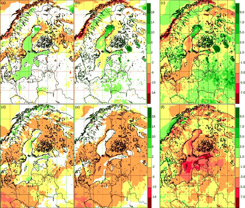
134                  O. B. Christensen et al.: Atmospheric regional climate projections for the Baltic Sea region until 2100

ever, not been addressed here as, at this point, downscaling       completely adequate as input to an RCM; this constitutes an
activities based on CMIP6 projections are still lacking.           additional source of potential uncertainty of the downscaled
   The Baltic Sea region is highly diverse with considerable       regional scenarios (Kjellström and Ruosteenoja, 2007).
spatial variability over small distances compared to typical          During the past decades, a number of regional coupled
GCM resolutions. Consequently, GCMs do not represent all           atmosphere–ocean–sea-ice models with focus on the Baltic
relevant processes at adequate scales and results are often        Sea and adjacent marginal seas have therefore been de-
biased (e.g. Graham et al., 2008). High-resolution regional        veloped for climate studies (e.g. Gustafsson et al., 1998;
climate models, nested in the GCMs, have been shown to             Döscher et al., 2002; Wang et al., 2015; Dieterich et al.,
add value to the GCM results and to promote detailed analy-        2019; Primo et al., 2019; Kelemen et al., 2019; Akhtar et al.,
sis on regional to local scales (e.g. Giorgi and Gao, 2018).       2019; Sein et al., 2020). In these models, prescribed bound-
At the European level, considerable efforts have therefore         ary conditions at the sea surface (i.e. sea ice and SST) were
been undertaken to downscale GCM simulations to a higher           replaced by online coupled ocean models allowing for a di-
horizontal resolution with RCMs. The history of coordi-            rect and more realistic representation of air–sea thermal feed-
nated RCM simulations started in the Prediction of Regional        back mechanisms (see review by Gröger et al., 2021b). These
Scenarios and Uncertainties for Defining European Climate          coupled models exhibit a different model solution for many
Change Risks and Effects (PRUDENCE) project with RCMs              climate variables compared to their atmosphere stand-alone
mostly operated at 50 km spatial resolution (Christensen and       counterparts, especially over the coupled region (Gröger et
Christensen, 2007), continued with the Ensemble-based Pre-         al., 2015; Ho-Hagemann et al., 2017; Primo et al., 2019;
dictions of Climate Changes and their Impacts (ENSEM-              Gröger et al., 2019, 2021a). The most recent and largest en-
BLES) project (van der Linden and Mitchell, 2009; Hanel            semble of regional coupled climate change simulations was
and Buishand, 2011; Kyselý et al., 2011; Räisänen and Ek-          provided by Dieterich et al. (2019) and Gröger et al. (2019,
lund, 2011; Déqué et al., 2012; Kjellström et al., 2013)           2021a), and is based on the Rossby Centre Regional Climate
and more recently in the EURO-CORDEX initiative, which             Model (RCA4) coupled interactively to the Nucleus for Eu-
forms part of the Coordinated Regional climate Downscal-           ropean Modelling of the Ocean (NEMO).
ing EXperiment (CORDEX, https://cordex.org/, last access:             Available RCM literature describes extensive studies of
14 January 2022; e.g. Giorgi et al., 2006; Jacob et al., 2014;     possible future climate conditions for many areas, including
Kotlarski et al., 2014; Keuler et al., 2016; Kjellström et         the Baltic Sea basin (see, e.g. Lind and Kjellström, 2008;
al., 2018). Most recently, the European Copernicus Climate         Kjellström and Lind, 2009; Benestad, 2011; Kjellström et
Change Services has supported an extension of the avail-           al., 2011; Nikulin et al., 2011; Christensen et al., 2015a;
able CMIP5-driven RCM downscaling simulations in the               Christensen and Kjellström, 2018; Coppola et al., 2021). En-
EURO-CORDEX setup with around 12 km spatial resolu-                sembles of climate projection simulations have been used to
tion (Vautard et al., 2021; Coppola et al., 2021). This has led    obtain probabilistic climate change information, both GCM
to the public availability of a large amount, currently 127,       (Lind and Kjellström, 2008; Räisänen, 2010) and RCM en-
of different simulations following the RCP2.6, RCP4.5, and         sembles (Buser et al., 2010; Donat et al., 2011). In addition,
RCP8.5 scenarios (some simulations with known errors are           the wider range of GCM scenarios has been used to set re-
not counted).                                                      gional scenarios in a broader context (Lind and Kjellström,
   Regional climate models have been used not only for             2008; Kjellström et al., 2016, 2018).
downscaling of climate change scenarios. Also, observation-           This work aims at presenting climate change in the area
based reanalysis datasets have been extensively downscaled         around the Baltic Sea, as it is projected by the very large en-
with RCMs in recent years (e.g. Feser et al., 2001; Hagemann       semble of EURO-CORDEX RCMs at 12 km resolution. The
et al., 2004; Christensen et al., 2010; Samuelsson et al., 2011;   spread in results between the projections is used to discuss
Kotlarski et al., 2014; Prein et al., 2015). These experiments     uncertainties in future climate change. In addition to the un-
are useful for comparing RCM results and observational data        coupled atmosphere-only EURO-CORDEX RCM ensemble,
for recent decades, and thereby for evaluation of RCM mod-         we will also assess changes in an ensemble with the atmo-
els. The RCMs are found to capture many features of the            spheric regional model RCA4 coupled to the NEMO ocean
climate in a realistic way, albeit with some systematic errors     model. A comparison between results from the stand-alone
and biases (Wibig et al., 2015; Kjellström and Christensen,        atmospheric model and the coupled model provides input to
2020). As a remedy, bias correction is sometimes applied           the assessment of uncertainties in future climate change pro-
to the results (e.g. Dosio et al., 2016). Biases are generally     jections for the area.
larger when GCMs are downscaled instead of reanalysis data,
as these show systematic biases in their representation of the
atmospheric circulation at large scales, of temperature, hu-       2   Data and methods
midity, and sea-surface conditions. For an area like the Baltic
Sea region, this implies that sea-surface temperatures (SSTs)      We will focus on data of the most commonly studied fields:
and sea ice from the coarse-scale driving GCM may not be           surface air temperature, average total precipitation, mean

Earth Syst. Dynam., 13, 133–157, 2022                                                https://doi.org/10.5194/esd-13-133-2022
O. B. Christensen et al.: Atmospheric regional climate projections for the Baltic Sea region until 2100                     135

wind speed at 10 m height, incoming short-wave radiation,        2009), consisting of simulations following the Special Report
and average winter snow and sea-ice cover. The conse-            on Emissions Scenarios (SRES) (Nakićenović et al., 2000)
quences of extreme weather events impact many aspects            A1B scenario performed in 25 km grid resolution. The peri-
of society. Extreme precipitation often results in flooding,     ods compared were 1961–1990 and 2071–2100. The mean
which often causes extensive damage as do extreme winds          GCM global temperature change weighted with the num-
in connection with low-pressure systems. Changes in these        ber of RCM simulations in the ensemble, for the EURO-
extremes as a result of anthropogenic climate change have        CORDEX and ENSEMBLES simulations, can be seen in Ta-
received considerable attention. We will therefore also report   ble 2. Note that the first reference period differs between
on extremes of daily precipitation and 10 m wind speed.          ENSEMBLES (1961–1990) and EURO-CORDEX (1981–
   The main results of this study build on seasonal means        2010).
from the publicly available and accessible EURO-CORDEX              To a high extent, maps over the Baltic Sea catchment of
data, which at the time of writing consisted of the 124 sim-     climate change for the weaker emission scenarios exhibit the
ulations indicated in Table 1 out of a current total of 127.     same patterns as the RCP8.5 climate change normalized by
Three different emission scenarios have been widely used for     global temperature change; maps are available in the Supple-
downscaling within CORDEX. The RCP2.6 scenario is the            ment.
most moderate and will require a targeted emission reduc-           The maps below show results based on 72 regional cli-
tion worldwide. The RCP8.5 scenario, in contrast, is consis-     mate change simulations from the RCP8.5 EURO-CORDEX
tent with large future increases in emissions, little emission   simulations listed in Table 1. Corresponding plots for other
mitigation, and a continued reliance on fossil fuels for many    scenarios and periods can be found in the Supplement. For
decades. In the middle, the RCP4.5 scenario requires a con-      each location, the median among ensemble members of the
siderable amount of mitigation but is very unlikely to achieve   change is shown together with the first and third quartiles.
the 2 % warming limit relative to pre-industrial conditions,     In the maps showing the median, we only display grid points
which the Paris Agreement targets.                               where 75 % of models agree on the sign, i.e. where both quar-
   In this study, we will concentrate on the warmer RCP8.5       tile plots show the same sign; elsewhere, we indicate in a
scenario. In the analysis, we will analyse three periods:        white colour that the changes are not robust. We will discuss
1981–2010, 2041–2070, and 2071–2100. Plots correspond-           only DJF and summer (JJA) in this study. The scatter plots
ing to the other scenarios can be found in the Supplement. In    below show results for all simulations following the three
general, the amplitude of regional climate change for varying    commonly used scenarios (Table 1). Where possible, we also
scenarios scales with temperature change, while the spatial      include results from the ENSEMBLES project, which were
pattern is similar (see, e.g. Christensen et al., 2015b). This   the basis of BACC II (Christensen et al., 2015a). In addition
means that the RCP8.5 scenario will show expected patterns       to the average over the entire Baltic Sea catchment region in-
of climate change with a relative minimum of noise from          cluding the Baltic Sea, we divide the region into sea points
interannual variability of the simulations. Furthermore, the     and land points north and south of 60◦ N. In the Supplement
largest of all three RCP ensembles is the RCP8.5 one (Ta-        (Tables S1–S20), tables of ensemble means and ensemble
ble 1); hence, the analysis of these scenario simulations al-    standard deviations can be found for temperature and precip-
lows the best estimate of model uncertainties and internal       itation, for both periods, all scenarios (including the BACC
variability.                                                     II/ENSEMBLES SRES A1B scenario), and all five areas.
   Not all EURO-CORDEX simulations have been analysed               We will also investigate the coupled-model ensemble with
for every variable considered here; two WRF361H simula-          RCA4-NEMO. RCA4 is set up for the EURO-CORDEX do-
tions do not contain solar radiation, and snow and sea ice       main with a horizontal resolution of ∼ 25 km and 40 vertical
from several simulations either do not exist in the archive      levels. NEMO simulates the hydrodynamics of the Baltic Sea
or have not been downloaded. Some simulations with the           as well as the North Sea at ∼ 3.7 km resolution and 56 ver-
Convection-Resolving Climate Model (crCLIM) are missing          tical levels (Gröger et al., 2015; Dieterich et al., 2019). Air–
winter (DJF) 2005–2006 due to a problem when handling the        sea fluxes are exchanged every 3 h between the ocean and
transition between historical and scenario simulations; we       the atmosphere. The RCA4-NEMO ensemble consists of 22
have repeated DJF 2004–2005 in its place. All simulations        downscaled GCM simulations based on eight different global
driven by Hadley Centre Global Environment Model version         models for the historical period and the RCP2.6, RCP4.5,
2 Earth system configuration (HadGEM2-ES) are missing            and RCP8.5 scenarios. In addition, there is also a reanalysis-
the year 2100; for these simulations, we have used 2070–         driven simulation for the historical period.
2099 as the end-of-century period.                                  These results will be compared to the corresponding
   The second Baltic Sea Experiment (BALTEX) Assessment          RCA4 atmosphere-only simulations at 12.5 km resolution,
of Climate Change for the Baltic Sea basin (BACC) report         which can be found in the EURO-CORDEX archive. When
from 2015 (BACC II Author Team, 2015) showed similar             possible, these simulations are included in the scatter plots
maps to those presented here. These results were based on        below.
the ENSEMBLES database (van der Linden and Mitchell,

https://doi.org/10.5194/esd-13-133-2022                                             Earth Syst. Dynam., 13, 133–157, 2022
136                   O. B. Christensen et al.: Atmospheric regional climate projections for the Baltic Sea region until 2100

Table 1. Model simulations of the study. These constitute the entire set of seasonal average fields available from the Earth System Grid
Federation (ESGF; http://esgf-data.dkrz.de, last access: 31 May 2021) archive in May 2021. There are 72 ensemble members following
RCP8.5, 22 following RCP4.5, and 30 following RCP2.6.

Table 2. Average global warming from driving GCMs in each scenario, weighted by the number of downscaling simulations of each. The
warming is presented relative to the reference period 1981–2010 for mid-century (2041–2070) and end-of-century (2071–2100) conditions.

                 Project              Scenario      Ensemble size    Mid-century warming      End-of-century warming
                 ENSEMBLES            SRES A1B                 13                        –                        3.00
                 EURO-CORDEX          RCP8.5                   72                     2.21                        3.71
                 EURO-CORDEX          RCP4.5                   22                     1.67                        2.13
                 EURO-CORDEX          RCP2.6                   30                     1.22                        1.19

Earth Syst. Dynam., 13, 133–157, 2022                                                     https://doi.org/10.5194/esd-13-133-2022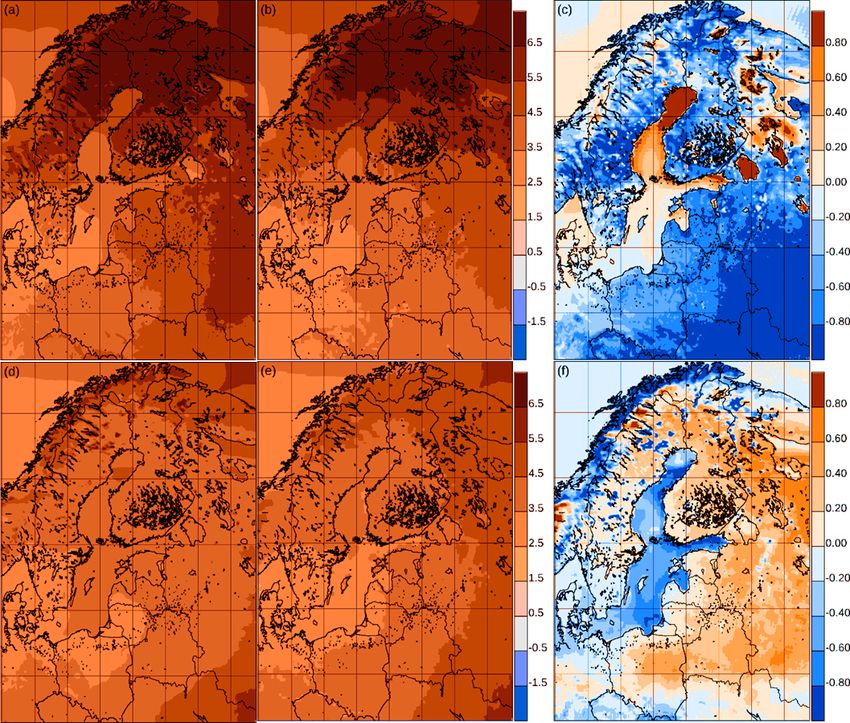
O. B. Christensen et al.: Atmospheric regional climate projections for the Baltic Sea region until 2100 137
3 Results and discussion increases further to the north in the Arctic, potentially con-
nected with the ice–albedo and other feedback mechanisms
3.1 Temperature (IPCC, 2021). The strong warming in the southeastern part
of the Baltic Sea basin is related to the large-scale pattern
According to the analysed EURO-CORDEX ensemble, we of warming in Europe, where the strongest summer warming
will see increasing air temperature in the Baltic Sea area dur- is seen in southern Europe. Similar results for other GCM–
ing the present century. According to this ensemble, it is a RCM combinations have been reached in, e.g. Christensen
robust result for all seasons, locations, simulations, and sce- and Christensen (2007), Kjellström et al. (2011), and Vautard
narios. et al. (2014). A potential source of difference between GCMs
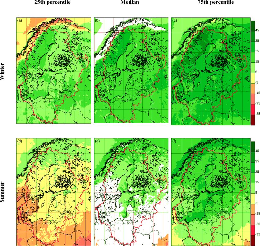
For both seasons analysed (winter and summer), the tem- and RCMs is the different treatment of aerosols in these mod-
perature change shows spatial gradients with the strongest els. Many of the RCMs do not include time-varying anthro-
warming in the northeast (Fig. 1). Winter warming is larger pogenic aerosols leading to weaker future warming com-
than summer warming and larger than the global average pared to GCMs (Boé et al., 2020). The EURO-CORDEX-
warming of about 3.7 % (Table 2); in the northeast, it ap- based results are consistent with the RCM results for 2021–
proaches twice the global average warming. Larger warm- 2050 in Déqué et al. (2012). This study found that there is
ing than the global average is generally expected for land ar- a significant temperature response, even for the relatively
eas, since land heats more quickly than sea areas where also short-term 2021–2050 time frame, even though the total un-
enhanced evaporation tends to reduce warming (e.g. Sutton certainty related to the choice of model combination (GCM–
et al., 2007); it is most clearly seen in winter in the eastern RCM) and sampling (natural variability) is large. Similarly,
part of the area. The strong winter increase is also influenced Kjellström et al. (2013) showed early emergence already in
by the feedback mechanisms involving retreating snow and the first few decades of the 21st century of trends in both win-
sea ice. There is a general pattern of higher warming in the ter and summer temperature despite large natural variability
north than in the south, but there is a spread in the mag- as represented in the ENSEMBLES RCM projections used
nitude of the change. This is illustrated in the columns of in BACC II.
the figures below. As only eight GCMs have been used for Corresponding changes in the daily minimum tempera-
these RCP8.5 RCM experiments, the spread between quar- ture and daily maximum temperature (not shown) have the
tiles could be lower than what would have come from an ex- same patterns as the average temperature change, with the
haustive downscaling of all CMIP5 global simulations; Kjell- expected larger magnitude of warming for minimum temper-
ström et al. (2016) compared nine GCMs, including the eight ature. A range of factors may be responsible for this decrease
GCMs analysed here, to 25 other CMIP5 GCMs and found in difference between minimum and maximum temperatures.
the nine-member-ensemble spread over Sweden to be com- This could involve changes in the diurnal temperature range
parable in summer but smaller than that in the larger GCM (e.g. Lindvall and Svensson, 2015) or changes in the synoptic
ensemble in winter. weather variability in combination with reduced large-scale
Earlier studies have shown that the increase in winter tem- temperature gradients between the Atlantic Ocean and the
peratures is strongest for the coldest episodes (Kjellström, Eurasian continent (IPCC, 2021).
2004) as well as for extreme daily maximum and minimum
temperatures (Kjellström et al., 2007; Nikulin et al., 2011). 3.2 Precipitation
There is a significant decrease in the probability of cold tem-
peratures (Benestad, 2011). Warm summer extremes are pro- The multi-model EURO-CORDEX ensemble relative precip-
jected to become more pronounced; for example, Nikulin itation change for winter and summer is shown in Fig. 2. The
et al. (2011) used an ensemble of six RCM simulations, all ensemble is the same as that in Fig. 1.
downscaling GCMs under the SRES A1B scenario; the data During winter, the relative increases are quite homoge-
indicate that warm extremes with a present-day (1961–1990) neous, although there are large differences between the lower
return period of 20 years will be reached 4 times as often and upper quartiles. These differences are largest west of the
in Scandinavia by 2071–2100, with a frequency around once Baltic Sea catchment (Norway) where the amount of pre-
every 5 years in Scandinavia by 2071–2100. cipitation is particularly sensitive to different changes in the
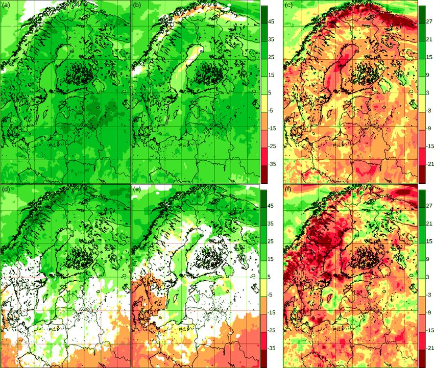
Summer warming in the Baltic Sea basin is smaller than large-scale circulation. For summer, there is a clear pattern of
winter warming, and it is relatively homogeneous across the more positive change in the north versus less positive change
area. A tendency is seen for larger warming over land ar- in the south. As expected, winter increases are projected to
eas in the northernmost parts of the Baltic Sea basin. These be larger than those in summer. Roughly, the winter increase
areas are closest to the northern rim of Scandinavia and is 25 %–35 % over most of the area in the median, and the
the Kola Peninsula where warming in summer is as high summer increase is 15 %–25 % for the northern part of the
as that projected for parts of southernmost Europe (Kjell- area. This is consistent with the AR5 Climate Atlas, where
ström et al., 2018). In the northeastern part of the region, median increases of precipitation in the area are 10 %–20 %
a large warming may be related to the larger temperature for the winter half year and 5 %–10 % for summer, as these
https://doi.org/10.5194/esd-13-133-2022 Earth Syst. Dynam., 13, 133–157, 2022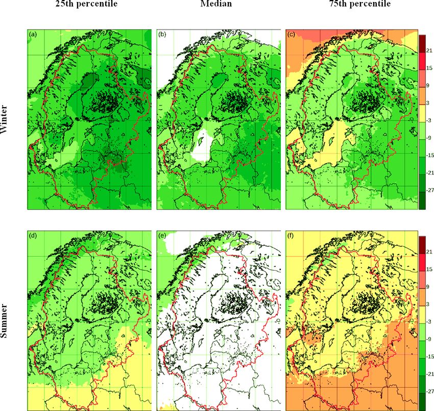
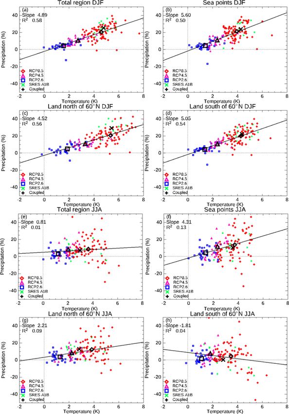
138                     O. B. Christensen et al.: Atmospheric regional climate projections for the Baltic Sea region until 2100

Figure 1. Temperature change between 1981–2010 and 2071–2100 for 72 simulations from EURO-CORDEX according to the RCP8.5
scenario. (a–c) Winter. (d–f) Summer. (a, d) Lowest quartile; (b, e) median value; (c, f) higher quartile. In all the following figures, panels (b,
e) depicting pointwise median values are only coloured when 75 % of the simulations agree on the sign of the change. The Baltic Sea
catchment is indicated in yellow.

results correspond to the RCP4.5 scenario with around 2.5 %                    This general picture of change is not surprising. Climate
of warming for the periods mapped, whereas the EURO-                        models generally project the global hydrological cycle to be-
CORDEX results correspond to a global warming of 3.8 ◦ C.                   come more intense (e.g. Held and Soden, 2006). For Europe,
   For summer, there is disagreement on the sign of climate                 this corresponds to increasing precipitation in northern Eu-
change for most of the southern half of the area, indicated by              rope and decreasing precipitation in southern Europe, both
the masked-out area defined as regions where at least 25 % of               in winter and summer (Christensen et al., 2007). Between
the models disagree on the sign with the majority. Since the                these areas of projected increase and projected decrease, only
period mapped here consists of the three summer months of                   small changes or changes in different directions are projected
June–August, whereas the AR5 Climate Atlas maps April–                      (see, e.g. Kjellström et al., 2011). The location of the tran-
September, a comparison of the position of the no-change                    sition zone depends on the season and is located farther to
area is difficult. In an analysis of the older ENSEMBLES                    the south in winter than in summer. In summer, this zone
simulations (Déqué et al., 2012), almost all land points in                 shifts into the Baltic Basin: winter precipitation is projected
the Baltic Sea region showed significantly positive summer                  to increase over the entire Baltic Sea catchment, while sum-
precipitation signals.                                                      mer precipitation is mostly projected to only increase in the

Earth Syst. Dynam., 13, 133–157, 2022                                                            https://doi.org/10.5194/esd-13-133-2022
O. B. Christensen et al.: Atmospheric regional climate projections for the Baltic Sea region until 2100                       139

northern half of the basin. In the south, precipitation change     larger increase of summer precipitation over the Baltic Sea.
is small for the ensemble mean, and there is a large spread        These conclusions do not contradict the results from Fig. 3,
between different models with both increases and decreases.        since a scaling with global warming would increase both lo-
Basically, both increases and decreases are possible in the        cal precipitation and local temperature changes for the BACC
future.                                                            II ENSEMBLES results relative to RCP8.5.
   In Fig. 3, we show scatter plots where the relative change
between 1981–2010 and 2071–2100 of precipitation is plot-          3.3   Extreme precipitation
ted against the corresponding change of temperature for each
model and each scenario. Ensemble means for the three sce-         The water-holding capacity of the atmosphere increases with
narios are indicated by the three larger symbols. This calcula-    increasing temperature. Therefore, precipitation extremes are
tion has been performed for various subsets of the Baltic Sea      projected to increase with climate warming (e.g. Lenderink
catchment (see Fig. 1): the entire region; only land points;       and van Meijgaard, 2010). Several studies, some of which
only sea points; only land points north and south of 60◦ N,        are described in the following, indicate that extreme precip-
respectively.                                                      itation is likely to increase in the future, even in areas and
   There is a strong correlation between temperature and           seasons, where the average precipitation does not increase.
precipitation in winter with significant regression slopes of      One example is the IPCC Special Report on extreme events
around five percentage points per degree and squared correla-      (Seneviratne et al., 2012), where it was shown that higher
tion coefficients of 0.5 to 0.6 depending on the sub-area. This    extremes of precipitation consistently show larger increases
is an indication of an approximate common sensitivity of           than lower extremes, and higher increases than averages.
precipitation change to local temperature change. This cor-           Already simulations from the PRUDENCE project (Chris-
respondence breaks down for summer, where the plots con-           tensen and Christensen, 2003) showing a considerable de-
tain much more noise, indicating large model-dependent in-         crease in average summer precipitation in large parts of
fluences on the precipitation signal. The north–south gradient     southern Europe at the same time showed an increased prob-
in summer precipitation change is apparent in the model av-        ability of very extreme precipitation in that area as well as
erages (compare the northern and southern land point plots),       in the north, where average precipitation was not projected
but the inter-model spread is large.                               to decrease. Quite generally, more intense precipitation can
   Due to the roughly 20 % higher average global warming in        be expected on all timescales, from single rain showers to
the current RCP8.5 ensemble than in the GCMs underlying            synoptic-scale precipitation.
BACC II (see Table 2), we would have expected general cli-            Nikulin et al. (2011) investigated an ensemble of RCM
mate change to be around 20 % larger for EURO-CORDEX               simulations following the SRES A1B scenario with the RCA
RCP8.5 than those presented in BACC II. It is noteworthy           model; they showed that the 20-year return value of precipi-
that this difference is not generally seen in Fig. 3, where        tation extremes in Scandinavia in the period 1961–1990 was
we have plotted temperature and precipitation change for the       projected to decrease to 6–10 years in 2071–2100 for sum-
BACC II simulations (BACC II Author Team, 2015) along              mer over northern Europe and to 2–4 years in winter. Simi-
with the three scenarios of the present analysis. The BACC         larly, Larsen et al. (2009) analysed a high-resolution RCM
II results correspond to the RCP8.5 results both with respect      integration and reported that the return period for 20-year
to temperature and precipitation change apart from land ar-        rainfall events at hourly duration decreased to about 4 years
eas in summer where the BACC II change is only about 80 %          for Sweden.
of the RCP8.5 result (+6.5 % vs. +8.2 %).                             Collected results from 90 of the models from the EURO-
   In Christensen et al. (2019), a thorough comparison of          CORDEX project are illustrated in Fig. 4, along with results
change patterns of mean temperature and precipitation has          from the coupled models discussed below. For data availabil-
been performed for the PRUDENCE simulations behind the             ity reasons at the time of writing, not all simulations have
first BACC report (BACC Author Team, 2008), the ENSEM-             been analysed for extreme precipitation. We will here use the
BLES simulations behind the second report (BACC II Au-             10-year return value as representative of extreme precipita-
thor Team, 2015), and the EURO-CORDEX data behind the              tion. This is defined as the daily precipitation amount, which
present report. This analysis used patterns of change scaled       is only exceeded once every 10 years on average. The model-
with global temperature change and is therefore useful for         median signal has a consistently positive sign across the do-
pinpointing differences between the BACC reports extrane-          main for the areas where more than 75 % of the model results
ous to the variations of general scenario strength, i.e. differ-   have the same sign. The temperature dependence of the in-
ences in local sensitivity and/or change patterns apart from       creases in the Baltic Sea basin (slopes in Fig. 4) are generally
those due to differences in emission scenarios. The most im-       larger in summer than in winter with the southern land points
portant differences between BACC II and the current sim-           as an exception, the same area where the average precipita-
ulations are a slightly reduced winter warming per unit of         tion (Figs. 2–3) decreases. The inter-model spread is consid-
global warming in EURO-CORDEX compared to BACC                     erably larger in summer than in winter, illustrating the greater
II; a smaller wintertime precipitation increase but a slightly     influence of local processes in this season; it should be noted

https://doi.org/10.5194/esd-13-133-2022                                               Earth Syst. Dynam., 13, 133–157, 2022
140                   O. B. Christensen et al.: Atmospheric regional climate projections for the Baltic Sea region until 2100

Figure 2. Precipitation relative change (%) between 1981–2010 and 2071–2100 for 72 simulations from EURO-CORDEX according to the
RCP8.5 scenario. (a–c) Winter. (d–f) Summer. (a, d) Lowest quartile; (b, e) median value; (c, f) higher quartile. In all following figures,
panels (b, e) depicting pointwise median values are only coloured when 75 % of simulations agree on the sign of the change. The Baltic Sea
catchment is indicated in red.

that the increase from 19 to 90 in the number of models anal-           cant for the average precipitation in summer. This feature is,
ysed, compared to Christensen and Kjellström (2018), results            however, less apparent in the EURO-CORDEX results than
in a considerably more robust positive signal in the summer             in the PRUDENCE results of BACC (BACC Author Team,
10-year return value.                                                   2008) and the ENSEMBLES results described in BACC II
   The relative changes of extreme precipitation in winter              (BACC II Author Team, 2015). It is not clear if this differ-
(Fig. 4 upper panels) are quite similar to the relative change          ence is due to the fact that the RCMs are run at different
in average precipitation (Fig. 2), indicating no change in              horizontal resolutions in the three projects (i.e. 50, 25, and
the shape of the intensity distribution function. For summer,           12.5 km, respectively), or if it is a consequence of different
however, the projected change in extreme precipitation is               model formulations in the projects or of the large-scale cli-
consistently more positive than the change in average precip-           mate change signal as imposed by the underlying GCMs that
itation. While the temperature sensitivities (slopes in Figs. 3         also differs between the experiments.
and 4) for winter average precipitation and winter extreme                 Recently, several research institutes have started employ-
precipitation are almost identical, the sensitivity of extremes         ing convection-permitting regional models (CPMs). Such
in summer is larger than that for winter, while it is insignifi-        models are able to run in much higher resolution, where tra-

Earth Syst. Dynam., 13, 133–157, 2022                                                       https://doi.org/10.5194/esd-13-133-2022
O. B. Christensen et al.: Atmospheric regional climate projections for the Baltic Sea region until 2100                                 141

Figure 3. Relative change 1981–2010 to 2071–2100 of precipitation against temperature change for individual models and all scenarios. Sce-
nario means are indicated by larger black symbols. Blue squares: RCP2.6; pink triangles: RCP4.5; red diamonds: RCP8.5; green crosses: the
ENSEMBLES simulations analysed in BACC II (2015). Plus signs in colours corresponding to the scenario: the RCA4-NEMO atmosphere–
ocean coupled simulations. Calculation performed for subsets of the Baltic catchment: the entire catchment; sea points; land points north and
south of 60◦ N, respectively. Panels (a)–(d) show winter; panels (e)–(h) show summer. The lines, with quoted slope and squared correlation
coefficient, are best fits to all EURO-CORDEX and ENSEMBLES data but do not include coupled-model results.

https://doi.org/10.5194/esd-13-133-2022                                                       Earth Syst. Dynam., 13, 133–157, 2022
142 O. B. Christensen et al.: Atmospheric regional climate projections for the Baltic Sea region until 2100
ditional hydrostatic RCMs with fully parameterized convec- area; the signal is consistent with the findings by Donat et
tive precipitation release may produce convective precipita- al. (2011) but with a large spread between models.
tion explicitly as well as parameterized, CPMs avoid this pos- Figure 5 shows average changes over the Baltic Sea for
sible double counting at high resolution. With CPMs grid dis- the 72 EURO-CORDEX RCP8.5 simulations, the 22 RCP4.5
tances below the “grey zone” of 3–5 km are possible. In Lind simulations, and the 30 RCP2.6 simulations, which were
et al. (2020), results are presented with the CPM HIRLAM used (Table 1). In Figs. S13–S18, we show median and quar-
ALADIN Regional Mesoscale Operational NWP in Europe - tile maps for summer and winter for each of the three RCP
Climate version (HARMONIE-Climate; HCLIM), produced scenarios. There is very little agreement between the models
in a common Nordic model collaboration (NorCP) with par- about even the direction of change for winter in the Baltic
ticipation from Sweden, Norway, Denmark, and Finland. Sea area unlike the tendency for reduced average wind speed
Comparing a CPM version of HCLIM in 3 km resolution outside of the study area over the North Atlantic (not shown).
with a non-CPM version in 12 km, it was concluded that Over the northernmost part of the Baltic Sea basin, the Both-
the high-resolution model showed better results for precip- nian Bay, there is an indication of larger wind speed in-
itation intensity distribution, including extreme precipitation crease (or less decrease) over the sea than over surrounding
at subdaily timescales, for the summer precipitation diurnal land areas. This feature has previously been pointed out by
cycle, and for snow in mountains. Such better agreement Kjellström et al. (2011), Meier et al. (2011), and Tobin et
now shown for the Nordic region has previously been shown al. (2016), and has been related to decreases in sea ice in the
for other regions in Europe and elsewhere (e.g. Kendon et future warmer climate, leading to consequent changes in sta-
al., 2014; Lind et al., 2016; Gao et al., 2020). bility conditions of the lower atmosphere. See also the com-
Based on convection-permitting models, it has been ar- parison between regional coupled and uncoupled simulations
gued that changes in precipitation extremes of a shorter in Fig. 12, where the probably more consistent treatment of
duration may be larger than those for longer timescales ice–albedo feedback leads to a slightly larger increase in win-
(e.g. Kendon et al., 2014; Lenderink and van Meijgaard, ter. As seen in Fig. 5b, the slight increase in mean wind over
2010). However, other results indicate (Ban et al., 2015) the Baltic Sea in BACC II is not projected in the current sim-
that convection-permitting models may give roughly the ulations.
same increase also for shorter durations, consistent with the Summer results show consistent but small reductions of
Clausius–Clapeyron scaling of around 6 %–7 % per degree wind over land of about 2 %–6 %. Again, in summer, there
of warming. In a study of idealized warming experiments are differences between land and ocean areas with generally
repeating present-day observed weather under warmer and larger increases, or smaller decreases, over the Baltic Sea
moister conditions with the HCLIM model, Lenderink et than its surrounding land areas.
al. (2019) showed that the increase in precipitation extremes The relative change in extreme wind speed is shown in
is strongly dependent on moisture availability. Fig. 6 as the relative change of the 10-year return value of
daily maximum wind speed for the EURO-CORDEX RCP-
based and the BACC II SRES-based simulations considered,
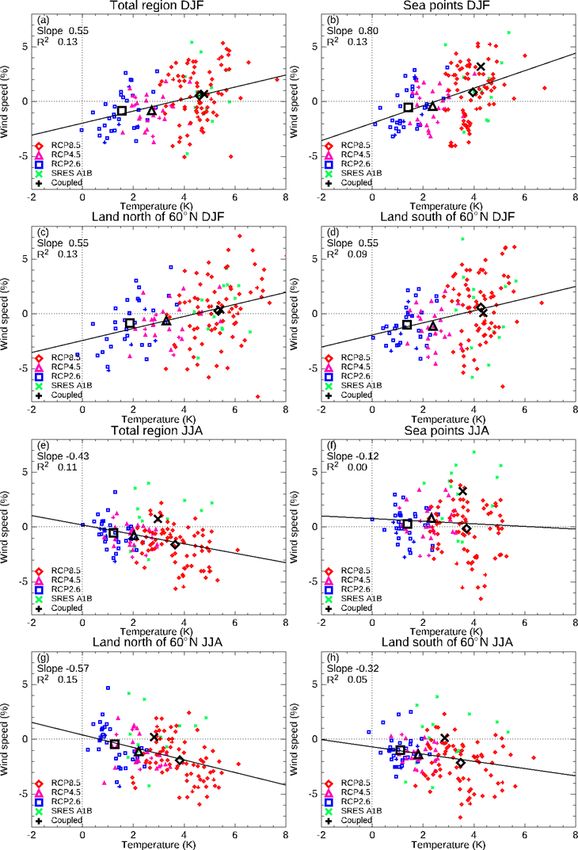
3.4 Wind speed as well as for the coupled RCA4-NEMO simulations. The
correlation between temperature and extreme wind is quite
Changes in the climatology of 10 m wind speed are even small, which indicates that there is no significant signal.
more uncertain than is the case for the precipitation cli-
mate, both for seasonal mean conditions and for extremes on 3.5 Solar irradiation
shorter timescales (e.g. Kjellström et al., 2011, 2018; Nikulin
et al., 2011). In Fig. 7, we study the change in incoming solar radiation
In a study by Donat et al. (2011), annual 98th percentile in the ensemble. In winter, most of the area shows a con-
daily maximum wind speed changes in RCM simulations siderable relative reduction of the order of 10 %. This has
from the ENSEMBLES project were analysed, for the mid- been proposed to be linked to the more extensive cloud cover
dle of the century as well as the end of the century. The en- in northern Europe in most EURO-CORDEX RCMs for the
semble average, like the driving GCMs, increased in a region future (Coppola et al., 2021). It should be noted (Bartók et
from the British Isles to the Baltic Sea and decreased in the al., 2017) that global and regional models frequently dis-
Mediterranean area. Nikulin et al. (2011) found increasing agree considerably about the change in incoming radiation in
wind speed extremes (20-year return periods of annual max- a changing climate, with global models having a more posi-
imum 10 m wind speed) over the Baltic Sea in five out of six tive trend; this discrepancy is connected to different projec-
simulations, based on an ensemble of one RCM downscaling tions of cloud cover, with GCMs frequently projecting a de-
six different GCMs under the A1B scenario. crease, while RCMs frequently show no significant change.
In BACC II (BACC II Author Team, 2015), an analysis of We repeat here that the different treatment of aerosols in
13 ENSEMBLES simulations showed a very small insignif- GCMs and RCMs plays a role as many of the RCMs do
icant median increase in the southern part of the Baltic Sea not include time-varying anthropogenic aerosols as in GCMs
Earth Syst. Dynam., 13, 133–157, 2022 https://doi.org/10.5194/esd-13-133-2022O. B. Christensen et al.: Atmospheric regional climate projections for the Baltic Sea region until 2100 143 Figure 4. Relative change 1981–2010 to 2071–2100 of the 10-year return value of daily precipitation against temperature change for indi- vidual models and all scenarios. Scenario means are indicated by larger black symbols. Blue squares: RCP2.6; pink triangles: RCP4.5; red diamonds: RCP8.5; green crosses: the ENSEMBLES simulations analysed in BACC II (2015). Plus signs in colours corresponding to the scenario: the RCA4-NEMO atmosphere–ocean coupled simulations. Calculation performed for subsets of the Baltic catchment: the entire catchment; sea points; land points north and south of 60◦ N, respectively. Panels (a)–(d) show winter; panels (e)–(h) show summer. The lines, with quoted slope and squared correlation coefficient, are best fits to all EURO-CORDEX and ENSEMBLES data but do not include coupled-model results. https://doi.org/10.5194/esd-13-133-2022 Earth Syst. Dynam., 13, 133–157, 2022
144                   O. B. Christensen et al.: Atmospheric regional climate projections for the Baltic Sea region until 2100

Figure 5. Relative change 1981–2010 to 2071–2100 of 10 m wind speed against temperature change for individual models and all scenar-
ios. Scenario means are indicated by larger black symbols. Blue squares: RCP2.6; pink triangles: RCP4.5; red diamonds: RCP8.5; green
crosses: the ENSEMBLES simulations analysed in BACC II (2015). Plus signs in colours corresponding to the scenario: the RCA4-NEMO
atmosphere–ocean coupled simulations. Calculation performed for subsets of the Baltic catchment: the entire catchment; sea points; land
points north and south of 60◦ N, respectively. Panels (a–d) show winter; panels (e–h) show summer. The lines, with quoted slope and
squared correlation coefficient, are best fits to all EURO-CORDEX and ENSEMBLES data but do not include coupled-model results.

Earth Syst. Dynam., 13, 133–157, 2022                                                    https://doi.org/10.5194/esd-13-133-2022
O. B. Christensen et al.: Atmospheric regional climate projections for the Baltic Sea region until 2100                                 145

Figure 6. Relative change 1981–2010 to 2071–2100 of the 10-year return value of 10 m daily maximum wind speed against temperature
change for individual models and all scenarios. Scenario means are indicated by larger black symbols. Blue squares: RCP2.6; pink triangles:
RCP4.5; red diamonds: RCP8.5; green crosses: the ENSEMBLES simulations analysed in BACC II (2015). Plus signs in colours correspond-
ing to the scenario: the RCA4-NEMO atmosphere–ocean coupled simulations. Calculation performed for subsets of the Baltic catchment:
the entire catchment; sea points; land points north and south of 60◦ N, respectively. Panels (a)–(d) show winter; panels (e)–(h) show summer.
The lines, with quoted slope and squared correlation coefficient, are best fits to all EURO-CORDEX and ENSEMBLES data but do not
include coupled-model results.

https://doi.org/10.5194/esd-13-133-2022                                                       Earth Syst. Dynam., 13, 133–157, 2022
146                   O. B. Christensen et al.: Atmospheric regional climate projections for the Baltic Sea region until 2100

Figure 7. Average incoming surface solar radiation relative change between 1981–2010 and 2071–2100 for 70 simulations from EURO-
CORDEX according to the RCP8.5 scenario. (a–c) Winter; (d–f) summer. (a, d) Lowest quartile; (b, e) median value; (c, f) higher quartile.
For the medians, only points where 75 % of models agree on the sign are shown. The Baltic Sea catchment is indicated in white.

(Boé et al., 2020). It has also been suggested that reduced            2010. Simultaneously, there is an increase in winter precipi-
snow cover (see Sect. 3.6 below) could contribute to attenu-           tation in Scandinavia, which may partly compensate for these
ate gross downward solar radiation flux as the reduced sur-            effects.
face albedo reduces multiple reflection between the surface               Räisänen and Eklund (2011) analysed data from RCM
and the clouds (Ruosteenoja and Räisänen, 2013).                       simulations from the ENSEMBLES project. The study found
                                                                       a decrease of snow volume across all of Europe in the fu-
                                                                       ture with the only exception that the Scandinavian moun-
3.6   Snow and sea ice                                                 tain areas may experience a slight and statistically insignif-
                                                                       icant increase. Räisänen (2021) found a widespread future
Future snow cover is expected to decrease with climate                 decrease in northern Europe for snow water equivalents also
warming, both because more precipitation is projected to fall          for a set of EURO-CORDEX RCMs. It was shown that a
as rain, and because snowmelt accelerates. As an indicator             smaller snowfall fraction together with larger reduction of
of less cold conditions, Coppola et al. (2021) show that the           snow on the ground more than compensated for increasing
number of frost days decrease by more than 2 months in                 precipitation, as seen in several of the RCMs. In relative
large parts of the Baltic Sea basin comparing a set of EURO-           numbers, the decrease was found to be larger in southern
CORDEX RCMs under RCP8.5 for 2071–2100 with 1981–

Earth Syst. Dynam., 13, 133–157, 2022                                                     https://doi.org/10.5194/esd-13-133-2022
O. B. Christensen et al.: Atmospheric regional climate projections for the Baltic Sea region until 2100 147 Figure 8. Relative change 1981–2010 to 2071–2100 of average winter (DJF) snow amount (kg/m2 ) against temperature change for 84 individual model simulations from all scenarios. Scenario means are indicated by larger symbols. Squares: RCP2.6; triangles: RCP4.5; diamonds: RCP8.5. Purple colour: the RCA4-NEMO atmosphere–ocean coupled simulations. Calculation performed for subsets of land points in the Baltic catchment: the entire catchment; land points north and south of 60◦ N, respectively. The lines, with quoted slope and squared correlation coefficient, are best fits to all EURO-CORDEX data but do not include coupled-model results. warmer parts of Scandinavia, while changes in absolute num- 2021). The reduction in snow amount is slightly larger than bers are larger in the north. Similarly, the results were am- in BACC II (BACC II Author Team, 2015). This is consis- biguous for the most high-altitude parts of the Scandinavian tent both with the fact that the RCP8.5 scenario on average mountains where some models indicate increasing snow wa- projects larger warming than the SRES A1B scenario used in ter and others a decrease. A potential increase in the latter BACC II and that the precipitation increase is smaller in the region was also proposed by Schuler et al. (2006) in a de- RCP8.5 scenario than in SRES A1B, at least north of 60◦ N tailed study for Norway based on two RCM simulations with (see Fig. 3c). different GCM drivers. The study concluded that the maxi- It is only in high-altitude parts of central and northern mum amount of snow in extreme years could be greater than Scandinavia that changes are limited with relatively large in extreme years of the recent past in spite of decreasing av- amounts of snow also in the future. At high altitude, the in- erage snow amount. crease of winter precipitation may be compensating for the Winter snow cover is one of the most drastically changed increase in melting with higher temperature. Also the fact climatological quantities (Fig. 8). There is agreement be- that increasing temperatures may not reach the melting point tween models about a reduction of average wintertime snow is significant; see, e.g. Gröger et al. (2021a) Fig. 12b. How- amount of around 50 % on average for land grid points north ever, also in these high-altitude regions, the warmer future of 60◦ N for the RCP8.5 scenario, and almost 80 % reduc- climate results in a shorter snow season with accumulation tion for land grid points south of this latitude. Northern grid starting later and spring melt starting earlier, which acts to points probably have a lower reduction due to the generally reduce the total amount of snow (Räisänen, 2021). colder climate and smaller amount of solar radiation. In ad- Sea-ice cover is not a product of the RCM but rather an dition, there is a significant amount of mountain grid points, input originating from the driving GCM. We will show the where the warming temperature does not reach the freez- changes in interpolated sea-ice field for the RCP8.5 scenario ing point as frequently as in lower-lying regions even if the in Fig. 9, as these changes are large and are decisive for the frequency is increasing in a warmer climate (Nilsen et al., change in climate between the periods. In order to compare https://doi.org/10.5194/esd-13-133-2022 Earth Syst. Dynam., 13, 133–157, 2022
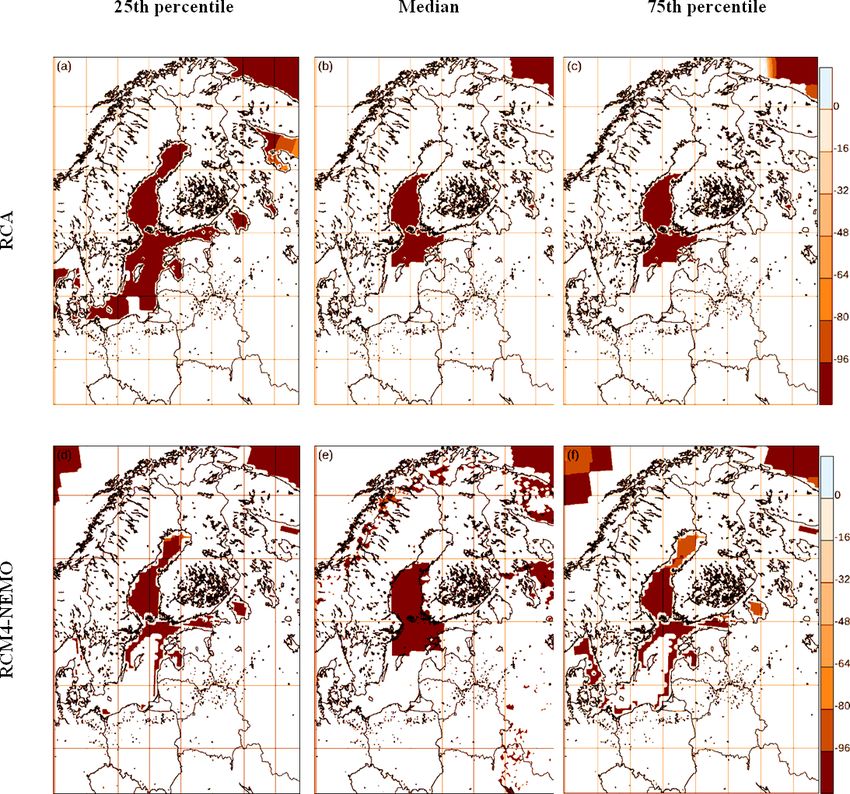
148 O. B. Christensen et al.: Atmospheric regional climate projections for the Baltic Sea region until 2100
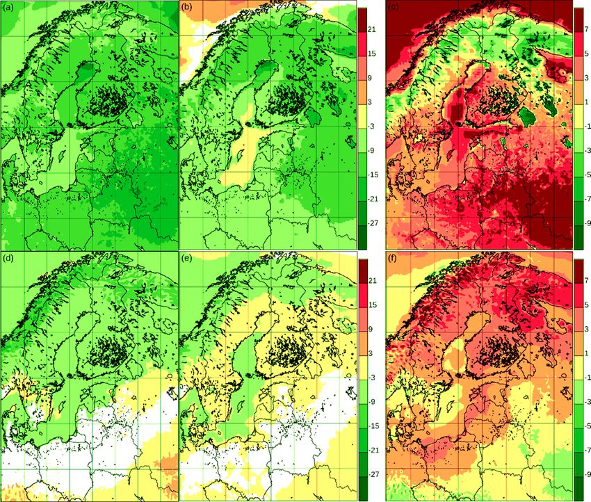
Figure 9. (a–c) Average winter sea-ice cover relative change between 1981–2010 and 2071–2100 for the simulations from EURO-CORDEX
according to the RCP8.5 scenario driven by the GCMs where RCA4-NEMO simulations exist. These values have been interpolated before
the RCM simulations from the driving coupled GCM; note that several simulations have sea ice in the Baltic Sea in the present-day period
but not in the Bothnian Bay. For comparison, in panels (d–f), we also show the corresponding fields from the corresponding five coupled
RCA4-NEMO simulations where sea-ice cover is calculated inside the regional model. (a, d) Lowest quartile; (b, e) median value; (c, f)
higher quartile. For the medians, only points where 75 % of models agree on the sign are shown.
to a more consistent description of sea ice, we also show For near-surface air temperature (Fig. 10), the large-scale
in Fig. 10 the corresponding figures for the eight-member anomaly pattern is fairly coherent in the two ensembles but
RCA4-NEMO coupled regional simulations. The main dif- differences are found over the northern Baltic Sea where the
ference is that the present-day simulations with the coupled coupled model shows a systematically stronger winter warm-
model have some extent of coastal sea ice in the southern ing than the uncoupled model. Over land, the coupled model
Baltic Sea, which is disappearing in the future. displays systematically lower warming. By contrast, during
summer the coupled model shows a weaker warming over
the entire Baltic Sea, while land temperatures increase more
than in the stand-alone RCA.
4 Effects of model coupling
Due to its higher effective heat capacity, the Baltic Sea
acts as a thermal buffer, which dampens the seasonal am-
Here, we take a more detailed look at RCM simulations plitude compared to the surrounding land areas. As a result,
driven by the five GCMs, which have been downscaled both the Baltic Sea is warmer than the overlying atmosphere dur-
by the stand-alone atmosphere EURO-CORDEX ensemble ing winter and releases heat to the atmosphere. Hence, in
and by the 24 km RCA4-NEMO coupled-model version (all regions not covered by sea ice, the SST significantly influ-
coloured squares in Table 1 for the RCA4 RCM).
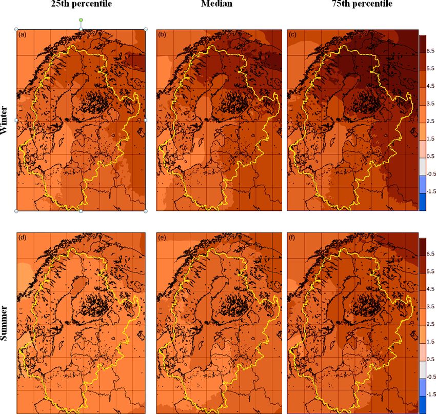
Earth Syst. Dynam., 13, 133–157, 2022 https://doi.org/10.5194/esd-13-133-2022O. B. Christensen et al.: Atmospheric regional climate projections for the Baltic Sea region until 2100 149 Figure 10. Temperature change between 1981–2010 and 2071–2100 for five atmosphere-only RCA4 simulations from EURO-CORDEX according to the RCP8.5 scenario (a, d) and for the coupled single-model RCA4-NEMO ensemble with the same driving GCMs (b, e); pointwise median values, only coloured when 75 % of simulations agree on the sign of the change. Difference between the two (c, f; coupled minus uncoupled; ◦ C). (a–c) Winter; (d–f) summer. ences the sea-to-air heat flux. Consequently, in the uncoupled GCM. Furthermore, changes in the mean and turbulent wind model, the prescribed SSTs from the driving atmosphere– stress due to local climate change in RCA have no impact on ocean GCM (AOGCM) serve as a restoring term for the air wind-induced mixing in the ocean in the RCA stand-alone temperature. By contrast, in the coupled model, SSTs are si- simulations. This further influences the local sea-ice cover multaneously modelled by the ocean model and so the air- and thus may explain the stronger warming over the northern to-sea heat transfer acts to cool SSTs until a new equilibrium Baltic Sea in the coupled model compared to the uncoupled would be reached. Despite these different dynamics in ther- version of RCA, which according to Fig. 9 generally starts mal coupling, over the southern Baltic Sea, the solution of the out with less sea ice in the present-day period and therefore two models is quite similar compared to the northern Baltic experiences less sea-ice loss. In the atmosphere, a stronger (Fig. 10). thermal coupling to the water body not only changes near- In the northern Baltic Sea, the reduction of sea ice has to be surface temperatures but also modifies atmospheric stability considered. In the future climate, areas which today are cov- and thereby mixing of heat, moisture, and momentum with ered by sea ice will get more tightly thermally coupled to the potential impacts on temperature, precipitation, and winds. water body of the Baltic Sea (Dutheil et al., 2022). As shown During summer when the Baltic Sea takes up heat from by Gröger et al. (2015, 2021a, b), the ocean-to-atmosphere the atmosphere, the air–sea heat exchange is greatly influ- heat transfer is largely affected by small-scale vertical mix- enced by the water bodies’ thermocline layer, which is of the ing in the layered ocean because wind-induced mixing trans- order of 10–30 m thick (e.g. Gröger et al., 2019). Thermo- ports warm waters from deeper water layers to the surface. cline dynamics is likely much more realistically represented These small-scale processes are most likely not well repre- when explicitly modelled by a coupled high-resolution ocean sented in the prescribed SST from the driving global ocean RCM rather than reflected in prescribed SST taken from a https://doi.org/10.5194/esd-13-133-2022 Earth Syst. Dynam., 13, 133–157, 2022
150                   O. B. Christensen et al.: Atmospheric regional climate projections for the Baltic Sea region until 2100

Figure 11. Precipitation relative change (%) between 1981–2010 and 2071–2100 for five atmosphere-only RCA4 simulations from EURO-
CORDEX according to the RCP8.5 scenario (a, d) and for the coupled single-model RCA4-NEMO ensemble with the same driving GCMs
(c, f); pointwise median values, only coloured when 75 % of simulations agree on the sign of the change. Difference between the two (c, f;
coupled minus uncoupled; %). (a–c) Winter; (d–f) summer.

global GCM of coarse resolution and only a few vertical lay-           sembles. A noteworthy difference between coupled and un-
ers (Gröger et al., 2015).                                             coupled simulations during winter is the stronger increase in
   Winter precipitation (Fig. 11) displays a fairly coherent           wind speeds over the Bothnian Bay. This points to local cou-
spatial pattern of change for the coupled and uncoupled RCA            pled feedback processes probably related to the vanishing sea
projections. However, the coupled model simulates system-              ice, higher sea-surface temperatures, and altered atmospheric
atically lower increases in precipitation than the uncoupled           static stability. A larger decrease in sea ice and a stronger
model. This is seen for both winter and summer. The differ-            coupling between the atmosphere and the water body leads
ences are most prominent over western Scandinavia and the              to a stronger heat flux to the atmosphere and thereby reduced
Bothnian Sea especially during summer.                                 vertical stability. This, in turn, leads to a more efficient down-
   A prominent feature of winter wind speed changes                    ward mixing of momentum in the lower atmosphere and con-
(Fig. 12) is the strong decrease along the Norwegian coast             sequently higher wind speed close to the sea surface.
seen in the coupled RCA model. This is also notable but                   The changes between future and present climate con-
less pronounced in the uncoupled runs. However, in those               ditions in solar irradiation (Fig. 13) are closely linked to
regions with steep topographic gradients, the differences can          changes in cloud cover. Both RCA versions simulate a gen-
be likely attributed to the differing grid resolutions though          erally less pronounced reduction in solar radiation during
coupling effects cannot be excluded. For most other land re-           winter than the average reduction seen in the entire EURO-
gions, winds are slightly weakened in the lower and slightly           CORDEX ensemble (Fig. 7). Strongest reductions are found
strengthened in the higher quartile, and a consequently high           over the Bothnian Bay in winter where vanishing sea ice ex-
uncertainty is seen for median winds (not shown). This is              poses open water to the atmosphere formerly isolated by sea
probably an effect of the different resolution of the two en-          ice. Compared to the coupled version, the uncoupled RCA

Earth Syst. Dynam., 13, 133–157, 2022                                                      https://doi.org/10.5194/esd-13-133-2022
You can also read