Multi-thermals and high concentrations of secondary ice: a modelling study of convective clouds during the Ice in Clouds Experiment - Dust (ICE-D) ...
←
→
Page content transcription
If your browser does not render page correctly, please read the page content below

Research article
Atmos. Chem. Phys., 22, 1649–1667, 2022
https://doi.org/10.5194/acp-22-1649-2022
© Author(s) 2022. This work is distributed under
the Creative Commons Attribution 4.0 License.

      Multi-thermals and high concentrations of secondary ice:
         a modelling study of convective clouds during the
         Ice in Clouds Experiment – Dust (ICE-D) campaign
          Zhiqiang Cui1 , Alan Blyth1,2 , Yahui Huang1 , Gary Lloyd2,3 , Thomas Choularton3 , Keith Bower3 ,
                                Paul Field1,4 , Rachel Hawker1 , and Lindsay Bennett2
                 1 Institutefor Climate and Atmospheric Science, University of Leeds, Leeds, LS2 9JT, UK
                               2 National Centre for Atmospheric Science, Leeds, LS2 9PH, UK
                  3 Centre for Atmospheric Science, University of Manchester, Manchester, M13 9PL, UK
                                              4 Met Office, Exeter, EX1 3PB, UK

                                   Correspondence: Zhiqiang Cui (z.cui@leeds.ac.uk)

                                    Received: 15 April 2021 – Discussion started: 27 May 2021
                      Revised: 2 December 2021 – Accepted: 17 December 2021 – Published: 3 February 2022

      Abstract. This paper examines the mechanisms responsible for the production of ice in convective clouds influ-
      enced by mineral dust. Observations were made in the Ice in Clouds Experiment – Dust (ICE-D) field campaign
      which took place in the vicinity of Cape Verde during August 2015. Measurements made with instruments on
      the Facility for Airborne Atmospheric Measurements (FAAM) aircraft through the clouds on 21 August showed
      that ice particles were observed in high concentrations at temperatures greater than about −8 ◦ C. Sensitivity
      studies were performed using existing parameterization schemes in a cloud model to explore the impact of the
      freezing onset temperature, the efficiency of freezing, mineral dust as efficient ice nuclei, and multi-thermals on
      secondary ice production by the rime-splintering process.
         The simulation with the default Morrison microphysics scheme (Morrison et al., 2005) that involved a single
      thermal produced a concentration of secondary ice that was much lower than the observed value of total ice
      number concentration. Relaxing the onset temperature to a higher value, enhancing the freezing efficiency, or
      combinations of these increased the secondary ice particle concentration but not by a sufficient amount. Simu-
      lations that involved only dust particles as ice-nucleating particles produced a lower concentration of secondary
      ice particles, since the freezing onset temperature is low. The simulations implicate that a higher concentration
      of ice-nucleating particles with a higher freezing onset temperature may explain some of the observed high con-
      centrations of secondary ice. However, a simulation with two thermals that used the original Morrison scheme
      without enhancement of the freezing efficiency or relaxation of the onset temperature produced the greatest con-
      centration of secondary ice particles. It did so because of the increased time that graupel particles were exposed
      to significant cloud liquid water in the Hallett–Mossop temperature zone. The forward-facing camera and mea-
      surements of the vertical wind in repeated passes of the same cloud suggested that these tropical clouds contained
      multiple thermals. It is possible of course that several mechanisms, some of them only recently discovered, may
      be responsible for producing the ice particles in clouds. This study highlights the fact that the dynamics of the
      clouds likely play an important role in producing high concentrations of secondary ice particles in clouds.

Published by Copernicus Publications on behalf of the European Geosciences Union.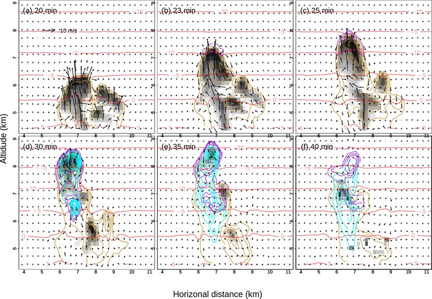
1650                                                                             Z. Cui et al.: Multi-thermals and secondary ice

1   Introduction                                                     contact freezing, and inside-out evaporation freezing (e.g.
                                                                     Cooper, 1986). Ice particles also form as a result of homo-
Ice particles in clouds contribute to the formation of more          geneous freezing at temperatures of about −40 ◦ C. The INP
than half of the world’s precipitation and greatly enhance the       concentrations are highly variable at a particular tempera-
amount of precipitation process over the warm-rain-only pro-         ture that depends on the dynamics and the aerosol properties
cess (McFarquhar et al., 2017). Precipitation in deep convec-        and humidity conditions. Most, if not all, models represent
tive clouds is closely related to the riming and melting of          the widespread relationships with parameterization schemes.
ice particles (Cui et al., 2011). Ice-phase processes in clouds      There is no one-size-fits-all solution to parameterize freezing
affect not only the weather, but also the climate, which is a        processes for all INPs.
new frontier of research in terms of aerosol–cloud–climate              Apart from the primary freezing processes, new ice crys-
interactions (Seinfeld et al., 2016; Storelvmo, 2017).               tals can be produced by secondary ice production (SIP) in
   Cloud drops form on cloud condensation nuclei (CCN)               the presence of preexisting ice without INPs. There are sev-
and primary ice particles on ice-nucleating particles (INPs).        eral SIP processes: fragments emitted from freezing large
The main INP types include mineral and desert dust, metals           drops (e.g. Wildeman et al., 2017), the mechanical break-up
and metal oxides, organics and glassy particles, bioaerosol,         of ice crystals by collision with other particles (e.g. Knight,
soil dust, biomass and fossil fuel combustion aerosol parti-         2012), splinter formation during the riming process (Hallett
cles, volcanic ash particles, and crystalline salts (Kanji et al.,   and Mossop, 1974), enhanced ice nucleation in regions of
2017). The onset and median freezing temperatures of those           spuriously high supersaturations (Hobbs and Rangno, 1990),
INPs show great intra- and inter-type variabilities (Kanji et        and ice particle fracture during evaporation of ice particles
al., 2017). An upper limit of the starting freezing temper-          (Oraltay and Hallett, 1989; Bacon et al., 1998). Of those pro-
atures of some bacteria INPs is typically between −2 and             cesses, the Hallett–Mossop (HM) parameterization has been
−4 ◦ C (Szyrmer and Zawadzki, 1997; Morris et al., 2004)             studied the most and is routinely incorporated into models.
and some even as high as −1.5 ◦ C (Kim et al., 1987; Lindow          New parameterizations for other mechanisms have been de-
et al., 1989). The activation temperature of mineral dust is         veloped recently (e.g. Phillips et al., 2017; Lawson et al.,
less than −15 ◦ C (Hoose and Möhler, 2012) but depends on            2017). Lawson et al. (2015) developed a parameterization for
their mineralogy (Murray et al., 2012). However, dust parti-         the drop-freezing secondary ice production process and sub-
cles can serve as INPs at higher temperatures if the fraction of     sequent riming. Lawson et al. (2017) developed an expres-
potassium-rich feldspar (K-feldspar) is high because feldspar        sion that predicts the level in the updraft core, where liquid
particles have high ice-nucleating active sites (Atkinson et         water becomes depleted. Observational and modelling stud-
al., 2013). A full functionalization of the ice-nucleating sites     ies have shown that the observed high ice concentration in
of a feldspar particle with hydroxyl groups enables a strong         some clouds may be explained by the Hallett–Mossop pro-
bonding to the prismatic plane of ice and prompts the for-           cess (e.g. Huang et al., 2008; Crosier et al., 2011; Crawford
mation of ice crystals on the surface of the feldspar (Kise-         et al., 2012; Huang et al., 2017; Hawker et al., 2021). For a
lev et al., 2017), which favours a higher freezing temper-           complete review of the literature on secondary ice produc-
ature. A recent study showed that a microcline mineral (a            tion, including the current state and recommendations for fu-
potassium-rich alkali feldspar) has bulk freezing tempera-           ture research, see Field et al. (2017), Korolev and Leisner
tures even greater than −3 ◦ C (Kaufmann et al., 2016). It has       (2020), and Korolev et al. (2020).
also been found that sea-spray aerosol particles can serve as           Many numerical models, including some cloud models, do
INPs (e.g. Wilson et al., 2015; DeMott et al., 2016), but they       not explicitly include the information about CCN and INP
do not act until the temperatures fall below −10 ◦ C. Burrows        but rather use parameterizations to represent a “general” or
et al. (2013) suggested strong regional differences in the im-       best-fit case for a freezing mode in the primary ice produc-
portance of marine biogenic INPs relative to dust INPs.              tion. As a result, a parameterized microphysics scheme does
   Nickovic et al. (2012) developed a high-resolution global         not reflect the aerosol environment of a cloud. Any depar-
dataset of mineral composition and showed the effective              ture of the INP properties from the best-fit condition, such
mineral content in soil for quartz, illite, kaolinite, smectite,     as the onset freezing temperature and the freezing efficiency,
feldspar, calcite, hematite, gypsum, and phosphorus. For ex-         may lead to an unrealistic representation of the cloud micro-
ample, the gradients of the surface content of feldspar are          physics.
particularly strong in the central Sahara. What makes the               Ice production in clouds is affected not only by microphys-
INPs even more complex is that they can be chemically and            ical processes, but also by cloud dynamics. Previous stud-
physically modified through chemical processing, internal            ies have revealed that thermals are the building blocks of
and/or external mixing, and cloud processing (Kanji et al.,          convective clouds (Koenig, 1963; Blyth and Latham, 1997;
2017).                                                               Keller and Sax, 1981; Damiani et al., 2006). The clouds of-
   Ice particles form via various primary pathways with the          ten contained multiple thermals that ascended in the wake of
help of INPs, such as deposition ice nucleation, contact freez-      their predecessors. In a theoretical study using a detailed mi-
ing, immersion freezing, condensation freezing, collisional          crophysics model in a simple dynamical framework, Blyth

Atmos. Chem. Phys., 22, 1649–1667, 2022                                               https://doi.org/10.5194/acp-22-1649-2022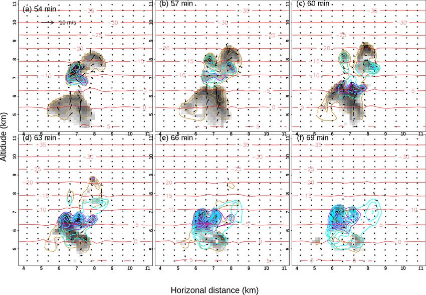
Z. Cui et al.: Multi-thermals and secondary ice                                                                                1651

and Latham (1997) found that multi-thermals can help yield          results. The final section provides the summary and conclu-
rapid ice HM multiplication by providing a new source of liq-       sions.
uid water content and by allowing the particles to be carried
by the thermal circulation. The results were consistent with
those found earlier by Koenig (1963) and others. The op-            2   Summary of the observations
eration of the HM process needs the coexistence of graupel,
large drops (> 25 µm), and small drops (< 12 µm) in the tem-        The observations of the ICE-D field campaign involved an
perature zone of −3 to −8 ◦ C. Previous studies have investi-       aircraft, radar, and ground-based measurements. The UK’s
gated the conditions favourable for secondary ice production:       FAAM BAe 146 research aircraft was used to conduct air-
moderate vertical velocities to allow graupel particles to fall     borne measurements of cloud microphysics and aerosol. A
into the HM zone and availability of both large and small           suite of instruments on board the BAe 146 measured the in-
drops for riming (e.g. Huang et al., 2008; Heymsfield and           formation about cloud microphysics, aerosol particles, and
Willis, 2014; Huang et al., 2017). It is important to consider      other atmospheric variables (see Price et al., 2018, Liu et
the possibility that multiple thermals will ascend through the      al., 2018, and Lloyd et al., 2020, for further descriptions).
HM zone because of the additional source of cloud drops that        One airborne aerosol instrument was the Passive Cavity
can rime onto graupel particles.                                    Aerosol Spectrometer Probe (PCASP), which can measure
   The field campaign of ICE-D (Ice in Clouds Experiment –          both aerosol number and size in the nominal size range 0.1 to
Dust) took place in the Cape Verde region, downwind of the          3 µm (Price et al., 2018; Liu et al., 2018). Ice particle concen-
African dust sources, in August 2015. Although there have           trations were derived from the two-dimensional stereo (2D-
been previous field campaigns that have investigated ice nu-        S) probe, an optical imaging instrument that obtains stereo
cleation in and near the Saharan region, most of them focused       cloud particle images and concentrations using linear array
on chemical and physical properties of the dust particles and       shadowing (Lawson et al., 2006; Cui et al., 2012, 2014).
their impact on large-scale phenomena (e.g. Knippertz et al.,       The UK Met Office ALS450 lidar manufactured by Leo-
2011; Rocha-Lima et al., 2018). ICE-D was specifically de-          sphere with an emitted wavelength of 354.7 nm and a re-
signed to study how dust affected ice production in convec-         ceiver bandwidth of 0.36 nm was on board the aircraft to
tive clouds using aircraft measurements, radar, and ground-         measure cloud-top height, range-corrected signal, and rela-
based aerosol instruments, which was complementary to a             tive depolarization ratio to map cloud and aerosol layers and
series of projects on layer clouds (ICE-L; see Heymsfield et        to retrieve aerosol optical properties (Marenco, 2013). A mo-
al., 2011) and tropical towering clouds (ICE-T; see Heyms-          bile dual-polarization Doppler X-band weather radar (Neely
field and Willis, 2014).                                            et al., 2018) of the National Centre of Atmospheric Science,
   Aircraft measurements were made by the Facility for Air-         UK, was deployed at the Praia airport on the island of Santi-
borne Atmospheric Measurements (FAAM) BAe 146 re-                   ago, Cape Verde. A suite of instruments was positioned at the
search aircraft on 21 August 2015 of convective clouds              airport to measure aerosol properties (Marsden et al., 2019).
about 150 km from the Praia airport, Cape Verde. There are             A trough existed along the western coast of Africa
two main points from the observations. Firstly, the maxi-           (Fig. 1a) on 21 August 2015. Convective cloud systems and
mum concentration of ice particles was greater than 200 L−1 ,       some smaller and more isolated convective clouds developed
greater than expected from INPs alone. Secondly, the first          along the coast. The aircraft operated in the region from
ice particles were believed to have formed at a temperature         longitude 23.541 to 21.022◦ W and from latitude 13.494 to
greater than about −5 ◦ C (Lloyd et al., 2020), which was           15.024◦ N. The operation region was characterized by rela-
thought to be a result of biological material either on or inter-   tively low aerosol optical depth (AOD) compared with the
nally mixed with the dust particles. This would mean that the       dust-plume region between −20 and −5◦ W and between 18
ice embryos would form at only slightly supercooled temper-         and 26◦ N (Fig. 1a). The aerosol subtype image by CALIPSO
atures (Obata et al., 1999; Lloyd et al., 2020).                    overpass to the west of the region indicates the existence of a
   In this paper, we report on a modelling study designed to        dust layer (in yellow) about 2 km thick (Fig. 1b). The aerosol
explore several aspects of the production of ice particles, that    below the dust layer was dominated by clean marine aerosol
is, the impact of the freezing onset temperature and the im-        with some polluted dust. Images from the onboard lidar show
pact of the efficiency of freezing in microphysics schemes,         that the range-correlated lidar signal, which is an indicator
to inspect the relationship between the measured dust as ef-        of aerosol loading, was much stronger below 1.5 km (all alti-
ficient INPs and the secondary ice production, and to in-           tudes are above mean sea level (MSL) in this paper) just after
vestigate the role of multi-thermals in producing high sec-         taking off. However, there was a layer with a slightly weaker
ondary ice concentrations. A three-dimensional cloud model          signal at about 2.3 km during the profile in Fig. 1c, which
was used for the simulations. Section 2 describes the obser-        was approximately 150 km to the west of the clouds shown
vations and datasets. The model description and numerical           in Fig. 1a. The relative depolarization ratio (spheres close to
designs are given in Sect. 3. Section 4 presents the simulation     0 and non-spheres much higher) indicates the aerosol par-
                                                                    ticles were soluble below 1.5 km within the boundary layer

https://doi.org/10.5194/acp-22-1649-2022                                            Atmos. Chem. Phys., 22, 1649–1667, 2022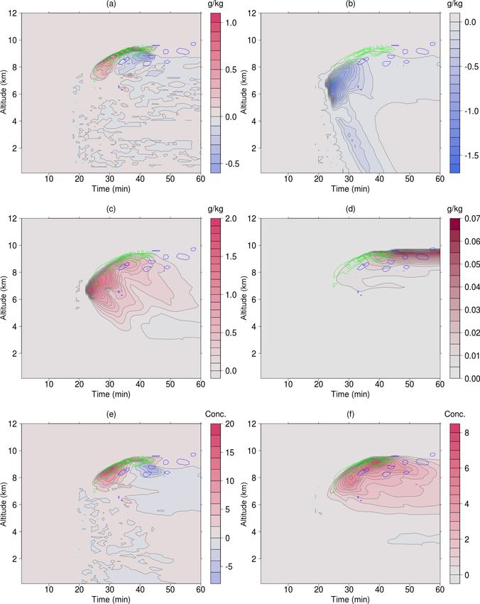
1652                                                                          Z. Cui et al.: Multi-thermals and secondary ice

and insoluble in the aloft layer (Fig. 1d). The lidar signals     −5 ◦ C, and the transition and interaction between different
were consistent with the PCASP measurement in Fig. 1e,            species.
which also shows the two aerosol layers. Together with the
CALIPSO image, we can conclude that the aloft aerosol layer       3.2   Experimental design
was mostly dust.
   The aircraft penetrated clouds between 100 and 300 km          One of the objectives of our study is to investigate the im-
to the south-east of Praia at various levels in the ambient       pact of the onset freezing temperature and the freezing ef-
temperature range of −1 to −7 ◦ C. In-cloud temperatures          ficiency on secondary ice production. As mentioned in the
could not be obtained because of wetting problems. The air-       introduction, the onset temperatures vary with the type of the
craft followed the ascending cloud top wherever possible and      INPs. The Morrison scheme uses the Cooper parameteriza-
made the passes a few hundred metres below the top in or-         tion (Cooper, 1986), in which freezing begins at a temper-
der to detect the formation and production of primary and         ature of −8 ◦ C. The temperature where freezing begins de-
secondary ice particles.                                          pends on the INP types. Recently, Garimella et al. (2018)
   Figure 2 shows the concentrations of ice particles in sev-     summarized some of the limitations of field measurements
eral passes based on the aircraft measurements. The max-          of INPs and their influence on the simulated cloud forcing in
imum concentrations of ice particles (i.e. non-spherical in       a global model. The parameterizations derived from field and
shape) in the size range of 50–1280 µm were 44 L−1 for a          laboratory data using the continuous-flow diffusion cham-
pass at −3.1 ◦ C (∼ 5500 m), 52 L−1 at −4.4 ◦ C (∼ 5800 m),       bers (CFDCs), for example, are subject to systematic low bi-
270 L−1 at −4.7 ◦ C (∼ 6100 m), and 82 L−1 at −6.8 ◦ C (∼         ases due to the limit of detection, not experiencing the max-
6500 m). As an example, the time series of concentration and      imum supersaturation, and the concurrence of ice particles
vertical velocity for the pass with the highest concentration     with drops. To reduce the bias, DeMott et al. (2015) proposed
is shown in Fig. 3. The observation indicates that the ice con-   applying a calibration factor of 3 to multiply the measured
centrations were a few tens per litre at derived temperatures     INP to obtain a better agreement. However, Garimella et al.
in cloud between 0 and −2 ◦ C (Lloyd et al., 2020). It is im-     (2017) noted that the calibration varied from 1.5 to 9.5 be-
possible of course to be certain of the origin of ice particles   cause of the lower relative humidity with respect to water
in such clouds. The fact that the passes were made within         than the intended values if aerosol deviated from the laminar
a few hundred metres of the cloud top, that the concentra-        flow, which indicates that this is one of the major problems
tions of ice particles were higher than expected from typical     in quantifying the formation of ice in numerical models.
INP measurements for the estimated cloud-top temperatures,           Considering these uncertainties, we investigate the in-
and that there was no evidence of higher concentrations of        fluence of the onset temperature and the efficiency in the
ice particles in the downdraughts suggest that secondary ice      ice production in sensitivity simulations using the Morrison
production most likely occurred.                                  scheme as the control run, where the initial drop number con-
                                                                  centration is 150 cm−3 . We also modify the Cooper param-
                                                                  eterization in the Morrison scheme with a parameterization
3     Cloud modelling                                             of DeMott et al. (2010) based on several datasets from dif-
                                                                  ferent regions as a function of temperature. A recently de-
3.1    Model description                                          veloped parameterization by Paukert and Hoose (2014) is
                                                                  also tested to probe whether dust INPs alone can produce
The Cloud Model 1 (CM1) was used for simulations in this          the concentration of ice observed by the aircraft. The details
study. More details on the model can be found in Bryan et         of the control and sensitivity tests are given in Table 1. The
al. (2003) and Bryan and Morrison (2012). The model uses          Morrison scheme has several ice freezing modes, including
conserved mass and energy conservation numerical schemes          immersion freezing, deposition freezing as a function of su-
in three dimensions and has a rich choice of microphysics         persaturation with respect to water and ice for this scheme,
schemes. In our simulations, the Morrison double-moment           contact freezing, homogeneous freezing, and the secondary
microphysics scheme (Morrison et al., 2005) was used to pre-      ice production by the HM process. For relaxation and en-
dict the mass ratio and the number concentration of cloud         hancement sensitivity simulations, we only modified the im-
droplet, rain, ice, snow, and graupel. The microphysical pro-     mersion freezing mode. The aims of the sensitivity simula-
cesses of drops include condensation, evaporation, collision      tions are summarized as follows. The early onset1 run ex-
and coalescence, sedimentation of cloud particles, and par-       amined the effect of active INPs at higher temperatures on
ticle growth by deposition of water vapour. The processes         secondary ice production when the onset temperature was
involved with ice include primary freezing modes of depo-         increased to −3 ◦ C. The Cooper10x run explored the effect
sition/condensation, contact, and immersion and secondary         of more INPs (i.e. the freezing efficiency was multiplied by
freezing through the rime-splintering (Hallett–Mossop) pro-       10). The early ohnset1 & Cooper10x run combined effects
cess (Hallett and Mossop, 1974; Cotton et al., 1986) in the       of the above two, while the early onset1 & 100xINP run
temperature range of −3 to −8 ◦ C, with a maximum at              and the early onset2 & 100xINP run probed the effect of

Atmos. Chem. Phys., 22, 1649–1667, 2022                                            https://doi.org/10.5194/acp-22-1649-2022
Z. Cui et al.: Multi-thermals and secondary ice                                                                                          1653

Figure 1. (a) MODIS combined Dark Target and Deep Blue mean AOD at 0.55 µm for land and ocean on 21 August 2015, with the red
line representing the path of the CALIPSO, (b) CALIPSO aerosol subtypes on 21 August 2015, (c) range-correlated lidar signal, (d) relative
depolarization ratio measured with the UK Met Office’s lidar on board the BAe 146 aircraft, and (e) vertical variation of aerosol concentration
measured with the PCASP on board the BAe 146 aircraft.

https://doi.org/10.5194/acp-22-1649-2022                                                   Atmos. Chem. Phys., 22, 1649–1667, 2022
1654                                                                                 Z. Cui et al.: Multi-thermals and secondary ice

Figure 2. Ice concentration as a function of altitude as measured
with the 2DS probe on board the BAe 146 aircraft. The colour bar
represents temperature.

                                                                        Figure 4. Initial profiles of (a) potential temperature and (b) mixing
                                                                        ratio for the model simulations. Altitude is the height above mean
                                                                        sea level.

                                                                        3.3    Model set-up

                                                                        The domain contained 100 × 100 grid points in the horizon-
                                                                        tal direction and 80 levels in the vertical direction, with a grid
Figure 3. Time series of the concentration of ice particles (L−1 ) in   spacing of 150 m in the three directions. The time step was
the size range of 50–1280 µm measured with the 2D-S Stereo Probe        2 s, and the output frequency was 1 min. Most of the simula-
and vertical velocity (m s−1 ) between 15:48:05 and 15:49:30 UTC        tions had a duration of 60 min, except for the multi-thermals
on 21 August 2015.                                                      and Paukert runs, which had a 120 min duration. The model
                                                                        was initialized with a horizontally homogeneous atmosphere
                                                                        (Fig. 4). Initial profiles of potential temperature and water
even higher loadings of INPs. The DeMott scheme (DeMott
                                                                        vapour mixing ratio were taken from measurements made by
et al., 2010) was examined in runs Demott, early Demott,
                                                                        radiosondes released from the aircraft in the vicinity of the
and Demott 10xINP. To investigate the effect of the dust as
                                                                        clouds studied. Because the release level of the dropsonde is
an INP, the Bigg (1953) scheme was replaced by the Pauk-
                                                                        lower than the highest level of the model domain, we used the
ert and Hoose scheme (Paukert and Hoose, 2014) since the
                                                                        NCEP/NCAR reanalysis data close to the cloud to represent
Bigg scheme does not consider INP types, but the Paukert
                                                                        the air above the radiosonde drop-off level. The simulated
and Hoose scheme considers different INP types. The Pauk-
                                                                        clouds were triggered by a warm bubble of 2 ◦ C in the con-
ert run used the mineral dust parameters in the Paukert and
                                                                        trol and most of the sensitivity runs except the multi-thermals
Hoose scheme. The Paukert-dust run was the same as the
                                                                        run, where another bubble was added 20 min from the start-
Paukert run except that the INP numbers were increased by
                                                                        ing time.
a factor of 3.3 in the layer between 2 and 3 km where the
coarse-mode concentrations in that dust layer were approxi-
mately 3.3 times higher than those above the layer (Fig. 1e).           4     Results
Finally, the effect of multi-thermals on secondary ice pro-
duction was examined in the multi-thermals when a second                4.1    Control simulation
bubble of 2 ◦ C was added after 20 min into the simulation.
                                                                        Figure 5 shows a time sequence of a cross section along the
                                                                        centre of the simulated cloud for the control run (control)

Atmos. Chem. Phys., 22, 1649–1667, 2022                                                    https://doi.org/10.5194/acp-22-1649-2022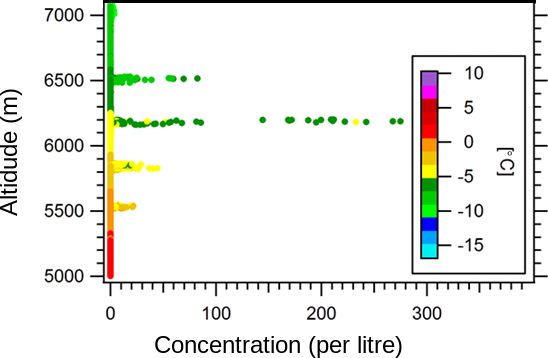
Z. Cui et al.: Multi-thermals and secondary ice                                                                                      1655

Table 1. Experimental design.

  Experiment                    Description
  Control                       The control run using the Morrison scheme
  Double-HM                     Same as control, except that the rate of the HM process is doubled.
  Early onset1                  Same as control, except that the onset freezing temperature is −3 ◦ C rather than −8 ◦ C.
  Early onset1 & noHM           Same as control, except that the onset freezing temperature is −3 ◦ C rather than −8 ◦ C, but switch off
                                the HM process.
  Cooper10x                     The ice nuclei number concentration from the Cooper scheme is multiplied by 10.
  Early onset1 & Cooper10x      Combination of early onset1 and Cooper10x
  Early onset1 & 100xINP        The onset freezing temperature is −3 ◦ C and the ice nuclei number concentration is multiplied by 100.
  Early onset2 & 100xINP        The onset freezing temperature is −2 ◦ C and the ice nuclei number concentration is multiplied by 100.
  Demott                        Use the DeMott et al. (2010) best fit, 0.117 exp(−0.125 × (T −273.2)), with the onset freezing temper-
                                ature being −8 ◦ C.
  Early Demott                  Same as Demott, but the starting freezing temperature is −3 ◦ C.
  Demott 10xINP                 Same as early Demott, but the ice nuclei number concentration is multiplied by 10.
  Paukert                       Paukert scheme
  Paukert-dust                  Same as Paukert, but the ice nuclei number concentration is enhanced in the dust layer.
  Multi-thermals                A second bubble of 2 ◦ C is imposed at 20 min from the simulation.

with only one thermal. The cloud ascended generally at a rate          to descend to about 8.5 km (T ∼ −18 ◦ C) by 40 min. The ice
of 300 m min−1 between 20 and 25 min. The maximum ver-                 crystal concentration increased to 21.5 L−1 at the cloud top.
tical wind was 17.7 m s−1 at 20 min and 8.3 m s−1 at 25 min;              The maximum values at each level in the control run of
thereafter, it ascended at a rate of about 150 m min−1 to              the vertical velocity and the number concentrations of rain-
36 min. The maximum vertical wind was 6.4 m s−1 at 30 min              drops, graupel particles, and ice crystals are shown in Fig. 6.
and 4.4 m s−1 at 35 min. The maximum level of the cloud top            As the cloud developed, latent heat release and reduced wa-
was 9075 m at 36 min. Figure 5a shows that there was a col-            ter loading drove the increase in the vertical velocity, and
umn of supercooled raindrops up to a temperature of about              the maximum reached 18.8 m −1 at z = 5.55 km at 19 min.
−5 ◦ C (6.3 km). There were no ice crystals or graupel parti-          Raindrops developed after 7 min, and the maximum concen-
cles. The cloud-top temperature was about −6 ◦ C at the time.          tration was 330.4 L−1 at z = 3.45 km at 13 min. The major
The cloud top reached around 8 km (T ∼ −14 ◦ C) at 25 min.             region of graupel particles appeared at an altitude of ap-
Ice particles were present in the upper 500 m with a maxi-             proximately 8 km at about 30 min, with the maximum being
mum concentration of 0.5 L−1 , but there were no graupel par-          1.7 L−1 at 8.7 km at 41 min. Additionally, a local maximum
ticles. The column of supercooled raindrops reached a tem-             was at about 6 km, and its value was 0.26 L−1 at 31 min. The
perature of about −14 ◦ C. There were few if any observations          major region of ice crystals occurred above an altitude of
of such cold columns, especially in tropical oceanic clouds.           8 km with a maximum of 21.5 L−1 at z = 9.15 km at 41 min.
At 30 min, the graupel particles fell into the HM zone, pre-           In the HM zone, the maximum concentration was 4.1 L−1 at
sumably around the edges of the thermal in the downdraughts            z = 6.6 km at 30 min, closely related to the local maximum
and then at the rear of the thermal, where the updraught is            in graupel concentration. Figure 6e and f show the variations
much weaker. The arrival of the graupel in the HM temper-              of the ice particle concentration of the early onset1 run and
ature zone allowed for splinters to be produced by the HM              the early onset1 & noHM run, respectively. The maximum
process. The graupel and ice concentrations in the HM zone             ice particle concentration in the HM zone of the early on-
reached 0.35 and 4.1 L−1 , respectively. The cloud had further         set1 simulation was 8.64 L−1 , while it was 0.27 L−1 in the
developed by 35 min such that the top had reached an altitude          early onset1 & noHM simulation, which clearly indicates the
of about 9 km (T ∼ −22 ◦ C), the maximum height. The con-              importance of rime splintering in the HM zone, where it is
centrations of ice in the HM zone and at the cloud top were            active more directly.
2.1 and 14.5 L−1 , respectively. By this time the entire cloud-
top region had begun to descend. The cloud top continued

https://doi.org/10.5194/acp-22-1649-2022                                                Atmos. Chem. Phys., 22, 1649–1667, 2022
1656 Z. Cui et al.: Multi-thermals and secondary ice
Figure 5. Time sequence for the control run control of spatial distribution of wind vectors, concentration of raindrops, ice crystals, and
graupel particles at (a) 20 min, (b) 23 min, (c) 25 min, (d) 30 min, (e) 35 min, and (f) 40 min. The orange, purple, and cyan lines are the
concentration of raindrops (contours at 1, then 2.5 to 10 in intervals of 2.5, and then in intervals of 5 to 70 L−1 ), ice crystals (contours at
0.25, 0.5, 1, 2.5, 5, 7.5, 10, 12.5, 15, 17.5, 20, and 22.5 L−1 ), and graupel particles (contour at 0.02 L−1 ), respectively. The shade represents
the cloud drop mixing ratio in each panel. The x axis and y axis are distance (km) and altitude (km), respectively. Also shown in each panel
are the maximum concentrations and scale of the wind vectors. Red lines are temperature in degrees Celsius.
4.2 Maximum concentration in the HM zone impact of possible INP properties, such as the onset freezing
temperature, the abundance of active INPs, and the freez-
Figure 7 shows the temporal variation of the maximum con- ing efficiency on the ice concentration in the HM zone, a
centration of ice in the HM zone for the control and sen- series of sensitivity simulations were conducted, as plotted
sitivity runs. Overall, the concentrations started to increase in Fig. 7. The maximum ice concentration was twice as high
at about 20 min and reached the maximum values at about when the rate of ice production in the HM scheme was dou-
30 min, except in the multi-thermals run. The curve of con- bled. When the onset freezing temperature of the Cooper pa-
centrations for the multi-thermals run was identical to that of rameterization in the Morrison scheme was relaxed from the
the control run before 45 min but greatly increases afterward. default value of −8 to −3 ◦ C (early onset1), the maximum
The control run produced a maximum ice concentration concentration increased to 8.8 L−1 . If the ice number con-
of 4.1 L−1 which was significantly smaller than the observed centration produced with the Cooper parameterization was
value (> 40 L−1 ). The Morrison microphysics scheme uses multiplied by 10 (Cooper10x), the maximum concentration
the Cooper parameterization for the primary ice production, increased to 13.4 L−1 . A combination of the relaxation and
which is based on a best-fit curve of measurements from enhancement (early onset1 & Cooper10x) further increased
Wyoming wintertime cap clouds, wintertime orographic the concentration in the HM zone to 30.6 L−1 . The maxi-
clouds of south-western Colorado, Israel winter cumulus mum concentrations increased to 45.3 L−1 in early onset1 &
clouds, summertime cumulus clouds of Montana, cumulus 100xINP and 48.6 L−1 in early onset2 & 100xINP. The De-
clouds of South Africa, and Australian cumulus clouds. As Mott scheme (Demott) produced the maximum concentration
discussed by Cooper (1986), the variance in the ice concen- of 11.7 L−1 . It increased to 32.2 L−1 with relaxation (early
trations at any given temperature is large, probably due to the Demott) and 40.4 L−1 with both relaxation and enhancement
high variability in the INP population itself or the wide vari- (Demott 10xINP).
ability in the activated fraction of INPs. Since the chemical The maximum concentration in the HM zone decreased
and physical properties of INPs vary with time and space, to 1.8 L−1 using the Paukert scheme (Paukert) when the
the Cooper parameterization does not necessarily represent Bigg (1953) scheme was replaced by the Paukert and Hoose
the INP conditions of the observed cloud. To investigate the
Atmos. Chem. Phys., 22, 1649–1667, 2022 https://doi.org/10.5194/acp-22-1649-2022Z. Cui et al.: Multi-thermals and secondary ice 1657
produce total ice concentration observed in some passes (e.g.
∼ 50 L−1 in pass at approximately 5830 m in Fig. 3) but
much lower than the maximum value ∼ 270 L−1 observed
in the cloud.
The temporal variations of the ice production in the HM
zone were broadly similar except for the two-thermal run
(multi-thermals) which produced a maximum concentration
of 121 L−1 at 69 min. We will discuss the causes of en-
hanced secondary ice production in the microphysical sen-
sitivity runs in Sect. 4.3–4.5.
4.3 Onset freezing temperature and freezing efficiency
Sensitivity tests were used to investigate the effect of varying
the onset freezing temperature and freezing efficiency on sec-
ondary ice production. The differences of several microphys-
ical properties between the sensitivity tests and the control
simulations are examined. There was a significantly higher
concentration of secondary ice particles produced in early
onset1 & Cooper10x compared with the control run. Fig-
ure 8 shows the detailed differences between the two runs. A
banana-shaped area of positive difference in vertical velocity
appeared in Fig. 8a. The positive region increased with time
and height from 23 min and z ∼ 6.6 km, reaching a maximum
concentration of about 2.7 m s−1 at 35 min at 9.15 km. The
increases in the vertical velocity were most likely caused by
Figure 6. Time–height variations of maximum values in (a) vertical the extra latent heat release due to the enhancement of freez-
velocity, (b) raindrop concentration, (c) graupel particle concentra- ing (e.g. McGee and van den Heever, 2014).
tion, (d) ice crystal concentration in the control run (control), as The region of the positive difference in the cloud water
well as (e) ice crystal concentration in the early onset1 run and (f) mixing ratio was well correlated with the enhanced vertical
ice crystal concentration in the early onset1 & noHM run. motion before 35 min, indicating that the enhanced vertical
velocity pushed the cloud top higher, which was confirmed
with an inspection of the fields of the two simulations and
their difference (figures now shown).
Although there was a small area of increase in the rain
mixing ratio, the ratio generally tended to decrease mainly
below 7 km and with the minimum at 24 min and z = 6.6 km.
The decrease was a result of more raindrops being converted
to graupel particles.
The maximum increase in the raindrop number concen-
tration in early onset1 & Cooper10x was at 30 min and
z = 8.55 km (Fig. 8e). However, a decrease occurred after
about 37 min, and the minimum is above 8 km. The positive
and negative regions shown in Fig. 8e are explained by the
fact that the concentration of raindrops was greater in the on-
set1 & Cooper10x run than in the control run up to about
Figure 7. Temporal variation of maximum concentrations of ice 38 min, and these drops remained elevated thereafter, while
crystals in the Hallett–Mossop temperature zone. those in the control run began to fall (figures not shown).
The mixing ratios of graupel and the ice crystals tended
to increase (Fig. 8c and d, respectively). The maximum in-
(2014) scheme (Paukert). Accounting for the dust layer creases appeared at 24 min and z = 6.75 km and at 47 min
(Paukert-dust) led to only a slight increase to 1.9 L−1 . and z = 9.45 km, respectively. The increase in the mixing ra-
Overall, the greater the starting freezing temperature, the tio of graupel seemed to be related to the raindrops being
higher the maximum ice concentration appears in the HM converted to graupel by direct freezing since there was no in-
zone. Simulations with both relaxation and enhancement can crease in ice particles at that time and altitude. The graupel
https://doi.org/10.5194/acp-22-1649-2022 Atmos. Chem. Phys., 22, 1649–1667, 20221658 Z. Cui et al.: Multi-thermals and secondary ice Figure 8. Difference between the sensitivity run early onset1 & Cooper10x and the control run control: (a) cloud water mixing ratio (g kg−1 ), (b) rain water mixing ratio (g kg−1 ), (c) graupel mixing ratio (g kg−1 ), (d) ice mixing ratio (g kg−1 ), (e) raindrop concentration (L−1 ), and (f) graupel concentration (L−1 ), respectively. Imposed on these figures are the differences in vertical velocity, with green contour lines indicating positive and blue contour lines negative differences and contour intervals of 0.5 m s−1 . number concentration increased (Fig. 8f), with the maximum With both relaxation and enhancement, the increase in the difference being at 39 min and z = 9.15 km. HM zone was 30.6 L−1 . The relaxation led to earlier sec- Differences in the maximum ice crystal concentration at ondary ice production and the enhancement increased ice each model level as a function of time between all the sensi- production not only in the HM zone, but also in the higher tivity runs and control are shown in Fig. 9. levels. The differences in concentrations further increased to For the early onset1 run, the differences at the upper lev- 45.2 L−1 in early onset1 & 100xINP and 48.5 L−1 in early els were small since the onset freezing temperature was only onset2 & 100xINP, as expected. There were more (fewer) in- relaxed from −8 to −3 ◦ C. However, the increase in the ice creases in the lower (upper) levels when using the DeMott crystal number concentration in the HM zone was 5.9 L−1 . scheme (Demott) because of the slope of the DeMott curve, For the enhancement run Cooper10x, the concentration in- i.e. more INP at higher temperatures. The ice concentration creased both in the upper levels and in the HM zone due in the HM zone in Demott was 11.6 L−1 . When the onset to more primary ice production, and the latter is 13.4 L−1 . freezing temperature was relaxed from −8 to −3 ◦ C (early Atmos. Chem. Phys., 22, 1649–1667, 2022 https://doi.org/10.5194/acp-22-1649-2022
Z. Cui et al.: Multi-thermals and secondary ice                                                                                 1659

                                                                       about 3 L−1 . This was because the onset freezing tempera-
                                                                       ture in the Paukert scheme was −12 ◦ C, less than the default
                                                                       value, −8 ◦ C, in the Morrison scheme. Freezing took place
                                                                       later in time and hence higher in altitude.
                                                                          To account for the dust layer between 2 and 3 km (Fig. 1),
                                                                       we increased the INP number to drop number ratio by a fac-
                                                                       tor of 3.3 in the Paukert scheme. However, the results indi-
                                                                       cate that there was an insignificant increase in the concentra-
                                                                       tion of ice particles (figures not shown). The results of these
                                                                       two simulations suggest that dust alone as a source of INPs
                                                                       was not enough to produce secondary ice concentrations that
                                                                       were similar to the observations in this case.

                                                                       4.5   Multiple thermals

                                                                       The above results indicate that the freezing rate and onset
                                                                       temperature in the Morrison scheme affect the secondary
                                                                       ice production. However, none of them produces a sufficient
                                                                       number of ice particles to explain the observations. Next, we
                                                                       will discuss the impact of cloud dynamics on the secondary
                                                                       ice production in a cloud with multi-thermals. It is important
                                                                       to consider both the dynamics and microphysics and their in-
                                                                       teractions since both play a critical role in ice production.
Figure 9. Difference in the ice crystal number concentrations (L−1 )   Figure 11 shows the time–height variations of maximum val-
between the sensitivity run and the control run: (a) early onset1,     ues of the vertical velocity, the raindrop concentration, the
(b) Cooper10x, (c) early onset1 & Cooper10x, (d) early onset1 &
                                                                       graupel particle concentration, and the ice crystal number
100xINP, (e) early onset2 & 100xINP, (f) Demott, (g) early Demott,
and (h) Demott 10xINP, respectively. The x axis and y axis are time
                                                                       concentration in the multi-thermals run.
(min) and altitude (km), respectively.                                    The defining feature of this run was the two updraughts
                                                                       (Fig. 11a). The isoline of 2 m s−1 of the first updraught
                                                                       started from the beginning at about 1 km and ended at about
Demott), there was a slight increase at the upper levels but a         35 min and reached an altitude of approximately 9 km, whilst
larger increase in the HM zone (32.1 L−1 ). With both relax-           the second started at about 20 min and also reached approxi-
ation and enhancement (Demott 10xINP), the increase in the             mately 9 km. There were no differences in the maximum ver-
HM zone was even larger (40.3 L−1 ) although not as large as           tical velocity in the first updraught before 20 min between
in early onset1 & 100xINP or early onset2 & 100xINP.                   the multi-thermals and control runs. The difference in the
   The results indicate that combinations of relaxing the onset        first updraught was minimal (< 0.5 m s−1 ) and appears be-
freezing temperature and enhancing the freezing efficiency             yond 20 min. Although the maximum vertical velocity in the
can produce secondary ice in concentrations of several tens            second updraught was smaller, the updraught lasted for ap-
per litre. However, these concentrations are significantly less        proximately 10 min longer than the first updraught.
than the maximum concentration observed by the aircraft.                  There was virtually no difference in the raindrop concen-
                                                                       tration associated with the first updraught. However, there
                                                                       were two local maxima associated with the second up-
4.4   Dust particles as INPs
                                                                       draught: one between 30 and 40 min at z = 2–4 km and the
It is interesting to consider whether it was possible to repro-        other between 50 and 60 min at z = 7–9 km. In the control
duce the observed concentrations of ice particles via primary          run, many raindrops precipitated before 20 min (Fig. 6b).
and secondary ice production processes if the INPs were                Some raindrops were transferred to graupel particles via di-
only dust particles. We used the Paukert scheme to address             rect freezing, but there were few raindrops remaining near the
this question with two simulations (see Table 1). The differ-          cloud top (e.g. Fig. 5c). In the multi-thermal run, the second
ences in the vertical velocity between the Paukert and con-            thermal started 20 min from the beginning. The lower-level
trol runs were less than 0.7 m s−1 (Fig. 10a). The number              maximum around 30–40 min was related to raindrops devel-
concentrations of raindrops, graupel particles, and ice crys-          oped with the second thermal. There was a second maximum
tals generally increased approximately above 8 km and de-              at z = 7–9 km (e.g. Fig. 12).
creased slightly below (Fig. 10b–d). There was less riming                There were very little differences in the graupel concen-
and therefore less secondary ice production in the HM zone.            trations between the multi-thermals run and the control run
The decrease in the ice concentration in the HM zone was               before 45 min by comparing Figs. 6a and 10a. However,

https://doi.org/10.5194/acp-22-1649-2022                                              Atmos. Chem. Phys., 22, 1649–1667, 2022
1660 Z. Cui et al.: Multi-thermals and secondary ice Figure 10. Difference between the Paukert run and the control run: (a) vertical velocity (m s−1 ), (b) raindrop number concentration (L−1 ), (c) the graupel concentrations (L−1 ), and (d) the ice crystal concentrations (L−1 ), respectively. two maxima appeared at 60 and 75 min between 7 and 8 km produced by the HM process. During the next 9 min, the co- with the multi-thermals run. The graupel concentrations were existence of graupel particles, drops, and raindrops produced much higher, 12 and 17 L−1 , compared with less than 2 L−1 secondary ice particles in the zone to 121 L−1 . More riming at about 40 min in the control run, which indicated more rim- and hence secondary ice particles were produced in the sec- ing in the multi-thermals run. Similarly, there were very little ond thermal due to the increase in liquid water content in the changes in the ice crystal concentration before 45 min. As- updraught. sociated with the two graupel maxima, there were two ice The results are consistent with the findings of Blyth and crystal maxima, one maximum being 84.9 L−1 at 58 min and Latham (1997) in that multi-thermals can significantly en- z = 6.9 km and the other maximum being 121 L−1 at 69 min hance the secondary ice production. A conceptual representa- and z = 6.75 km. tion of the kinematics was used in the detailed microphysics Figure 12 presents a time sequence of cloud properties for model described by Blyth and Latham (1997), whilst the the multi-thermals run between 54 and 69 min at intervals of present study employed a cloud model with detailed cloud 3 min spanning a period of a maximum of the secondary ice microphysical processes. There have been a few studies of production in the HM zone. thermals in shallow convective clouds (e.g. Heus et al., 2009; A turret containing graupel reached just above 8 km at Heiblum et al., 2016). It is impossible to make a direct com- x ≈ 7 km with strong updraught up to 7.6 m s−1 and rain- parison of thermals between the deep convective cloud in this drops below the turret at 54 min. The turret developed to a paper and those shallow clouds, but similar features were slightly higher level at 57 min and started to collapse, but found, such as enhanced vertical velocities and cloud mass strong updraughts of 7.8 m s−1 below the turret still sup- associated with the thermals. The injection time of 20 min ported the graupel particles from falling into the HM zone. was chosen when the updraught was about to decay (Fig. 11). As the turret continued to collapse and the updraughts below An earlier injection time (e.g. 10 min) of the second bubble the turret weakened, graupel particles fell down into the HM only slightly increased the first main updraught and did not zone at 60 min. A local maximum of ice concentration ap- change the result significantly. peared around 7 km in altitude and x ≈ 7.2 km, which was Atmos. Chem. Phys., 22, 1649–1667, 2022 https://doi.org/10.5194/acp-22-1649-2022
Z. Cui et al.: Multi-thermals and secondary ice                                                                                        1661

Figure 11. Time–height variations of maximum values in vertical velocity (a), raindrop concentration (b), graupel particle concentration (c),
and ice crystal concentration (d) in the two-thermal run (multi-thermals).

5   Discussions                                                          collision mechanism. Images of ice with irregular shapes are
                                                                         most likely produced by the drop shattering during freezing
                                                                         (Field et al., 2017).
Firstly, we discuss whether the conditions for the rime-                    Another question is whether very active (e.g. biogenic)
splintering process were met in cloud penetrations. Figure 13            INPs existed in the environment of the observed clouds
shows the variations of the aircraft-measured vertical ve-               (Lloyd et al., 2020). As described in Sect. 2, the aerosol parti-
locity and the cloud drop concentration at 6180 m between                cles in the lowest 1.5 km were mostly marine with some pol-
15:12:07 and 15:15:39 UTC. The vertical velocities indicate              luted dust, and the upper layer at 2–3 km consisted mostly of
the weak updraught in the cloud was surrounded by down-                  dust. The laser ablation aerosol particle time-of-flight mass
draughts. The vertical velocities were approximately 2 m s−1             spectrometer (LAAPTOF) was deployed to measure aerosol
at the time when columns were measured (Fig. 14). The con-               properties during the field campaign. The organic–biogenic
centrations of drops in the cloud were a few tens per cu-                fractions were moderately high in the measured dust parti-
bic centimetre (Fig. 13c). In Fig. 14, graupel particles, small          cles at the Praia airport on 21 August (Marsden et al., 2019),
droplets, and large drops were observed during the same pass             which could affect the ice formation in the clouds. Although
as in Fig. 13. Fragments of frozen drops were found, but not             the ground measurement site was about 150 km away from
in a great amount compared with the amount of columnar                   the clouds, it is possible that aerosol particles in the aircraft
crystals, although the exact concentration needed to be de-              operation region had a similar chemical composition to those
termined. The high concentrations of ice particles were most             at the ground site.
likely produced by the rime-splintering process because all                 It is noted that other mechanisms of secondary ice pro-
the conditions for the process were met. However, there is no            duction may have operated in these clouds, such as frag-
causal evidence of other mechanisms of secondary ice pro-                mentation during evaporation (Bacon et al., 1998), crystal–
duction. Qu et al. (2020), for example, showed that several              crystal collision (Takahashi et al., 1995), fragile needles com-
SIP mechanisms can operate within a convective cloud. Evi-               bined with ice–ice collision fragmentation (Knight, 2012),
dence of other secondary ice mechanisms could be provided                and shattering following the freezing of supercooled rain-
by cloud particle images. For example, images of fragmented              drops (Leisner et al., 2014; Wildeman et al., 2017). The shat-
ice, especially pieces of dendrites, are related to the ice–ice

https://doi.org/10.5194/acp-22-1649-2022                                                  Atmos. Chem. Phys., 22, 1649–1667, 2022
1662 Z. Cui et al.: Multi-thermals and secondary ice
Figure 12. Time sequence for the multi-thermals run of spatial distribution of wind vectors, concentration of raindrops, ice crystals, and
graupel particles at (a) 54 min, (b) 57 min, (c) 60 min, (d) 63 min, (e) 66 min, and (f) 69 min. The orange, purple, and cyan lines are the
concentration of raindrops (intervals at 2 L−1 ), ice crystals (intervals at 10 L−1 ), and graupel particles (intervals at 2 L−1 ), respectively.
Cloud drop mass mixing ratio is shown in shade in each panel. The cyan lines are isotherms in degrees Celsius. The maximum concentrations
are shown in each panel in L−1 . The scale for the wind vectors is also shown in (a).
can investigate the relative importance of this mechanism us-
ing new parameterizations accounting for the ice–ice colli-
sion processes (e.g. Phillips et al., 2017). Since the tops of
the clouds in this study were no higher than −10 ◦ C and the
conditions in the clouds were conducive to the HM process
as currently understood, we have focussed on modelling the
production of ice particles by that rime-splintering process.
The recent development of the parametrization of secondary
ice particles from frozen drops by Phillips et al. (2017) in-
dicates that this process might have a considerable contribu-
tion to the secondary ice formation at temperatures greater
than −10 ◦ C. Future research will undoubtedly include this
parametrization. It should also be noted that research con-
tinues on mechanisms that can cause an enhancement of ice
particles (e.g. James et al., 2021).
Figure 5a shows that the cloud model produced several
separate thermals over the approximately 4 km width of the
Figure 13. Variations of (a) the vector winds and (b) cloud drop cloud system. Only one of them (between 6 and 7 km) de-
concentration measured with the Cloud Drop Probe. veloped and ascended to 9 km. As discussed by Heus et al.
(2009), the inflow of air from the subcloud thermal is as-
sumed to be in balance with detrainment from the cloud
tering mechanism may be most efficient between −10 and into the environment in a mature cloud. In a single cloud
−15 ◦ C, and ice fragments generated by shattering may be simulation, a cloud is triggered by perturbations in tem-
transferred to lower or higher altitudes due to the updraughts perature as a thermal. Since the lower boundary conditions
and downdraughts. The Knight mechanism (Knight, 2012) were prescribed and only random perturbations were added,
operates at a similar temperature range, and future studies there were no subsequent thermals to produce profound heat
Atmos. Chem. Phys., 22, 1649–1667, 2022 https://doi.org/10.5194/acp-22-1649-2022Z. Cui et al.: Multi-thermals and secondary ice 1663
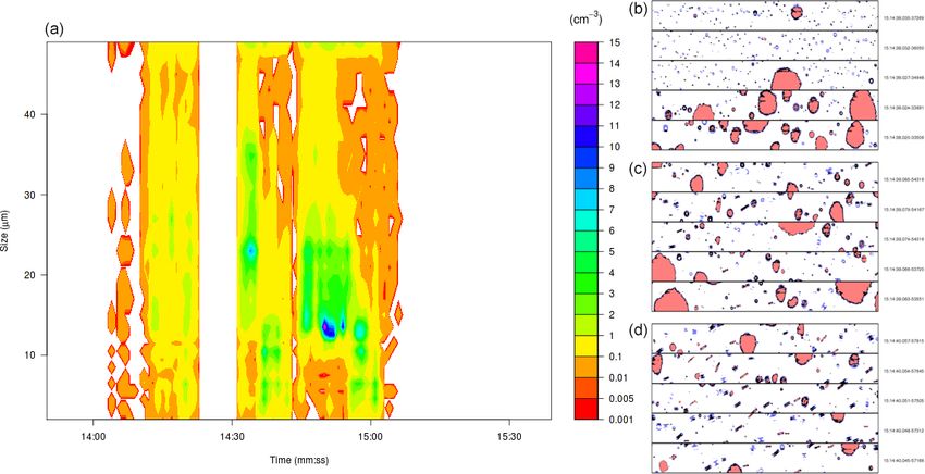
Figure 14. (a) Size distribution of drops measured with the Cloud Drop Probe and (b) examples of images measured with the Cloud Imaging
Probe (CIP) during Run 6. The CIP image width is 960 µm.
or momentum fluxes from the underlying surface that were of updraft velocities and horizontal extent. Initial conditions
strong enough to produce more new cloud droplets near the not only affect the thermodynamic environment of a cloud,
cloud base. Recently, Heiblum et al. (2016) simulated the but also directly affect ice nucleation and rime splintering.
cumulus field using a LES model and showed a series of in- Therefore, it is important to use the aircraft measurement of
cloud positively buoyant thermals spanning 5–15 min each in temperature and moisture profiles close to the clouds to be
precipitating clouds (their Fig. 3). However, there was only simulated.
one thermal in the non-precipitating cases. Their results indi-
cated that their multi-thermals could be a result of cold pool
interaction and subsequent lifting. The multi-thermal in con- 6 Conclusions
vective clouds could be topographically or thermally forced
in the mountainous region. In principle, NWP or cloud mod- Numerical simulations of the 21 August 2015 ICE-D deep
els will be able to describe the appearance of sequential ther- convective clouds in the Cape Verde region examined the
mals if the boundary layer conditions are realistically rep- secondary ice production through the rime-splintering pro-
resented. This study and previous studies by Ludlam and cess and the sensitivity to the onset freezing temperature
Scorer (1953), Koenig (1963), and Mason and Jonas (1974) or/and freezing efficiency as well as the impact of multiple
have highlighted the importance of atmospheric models be- thermals.
ing able to simulate these entities. CM1 was run for the 21 August case. The default Mor-
The behaviour of a simulated cloud is sensitive to the ini- rison microphysics scheme was applied for the simulations.
tial conditions. A perfect initialization requires one to follow Additional simulations were run with adjusted onset freez-
the trajectory of the cloud in time and space to get the ver- ing temperature, freezing efficiency, the Paukert scheme for
tical variation of thermodynamic variables before its forma- dust-only INPs, and a two-thermal simulation. The control
tion. The initial conditions we could get in close proximity simulation produced a maximum concentration of secondary
to reality were from the aircraft profile run after it took off to ice of a few per litre in the HM temperature zone which is
reach the clouds. The initialization based on the combination much lower than the observed value. One possible reason for
of aircraft measurement and reanalysis was a source of un- the underestimation is that the default onset freezing temper-
certainty. However, the major conclusion of this study is that ature is −8 ◦ C, which means the first ice in the control run
the multi-thermal is the only way to get enough ice. The ini- appeared too late at higher levels. Relaxing the onset temper-
tial conditions only have to be roughly correct to get a cloud ature from −8 to −3 ◦ C doubled the maximum concentra-
that goes to the correct height and has the same magnitude tion of the secondary ice but is still not as high as observed.
Enhancing the freezing efficiency made more primary ice
https://doi.org/10.5194/acp-22-1649-2022 Atmos. Chem. Phys., 22, 1649–1667, 2022You can also read