Uncertainties in eddy covariance air-sea CO2 flux measurements and implications for gas transfer velocity parameterisations
←
→
Page content transcription
If your browser does not render page correctly, please read the page content below

Atmos. Chem. Phys., 21, 8089–8110, 2021
https://doi.org/10.5194/acp-21-8089-2021
© Author(s) 2021. This work is distributed under
the Creative Commons Attribution 4.0 License.

Uncertainties in eddy covariance air–sea CO2 flux measurements
and implications for gas transfer velocity parameterisations
Yuanxu Dong1,2 , Mingxi Yang2 , Dorothee C. E. Bakker1 , Vassilis Kitidis2 , and Thomas G. Bell2
1 Centre   for Ocean and Atmospheric Sciences, School of Environmental Sciences, University of East Anglia, Norwich, UK
2 Plymouth    Marine Laboratory, Prospect Place, Plymouth, UK

Correspondence: Yuanxu Dong (yuanxu.dong@uea.ac.uk) and Mingxi Yang (miya@pml.ac.uk)

Received: 10 February 2021 – Discussion started: 19 February 2021
Revised: 18 April 2021 – Accepted: 21 April 2021 – Published: 26 May 2021

Abstract. Air–sea carbon dioxide (CO2 ) flux is often indi-     1   Introduction
rectly estimated by the bulk method using the air–sea dif-
ference in CO2 fugacity (1f CO2 ) and a parameterisation        Since the Industrial Revolution, atmospheric CO2 levels have
of the gas transfer velocity (K). Direct flux measurements      risen steeply due to human activities (Broecker and Peng,
by eddy covariance (EC) provide an independent reference        1998). The ocean plays a key role in the global carbon cycle,
for bulk flux estimates and are often used to study processes   having taken up roughly one-quarter of anthropogenic CO2
that drive K. However, inherent uncertainties in EC air–sea     emissions over the last decade (Friedlingstein et al., 2020).
CO2 flux measurements from ships have not been well quan-       Accurate estimates of air–sea CO2 flux are vital to forecast
tified and may confound analyses of K. This paper evalu-        climate change and to quantify the effects of ocean CO2 up-
ates the uncertainties in EC CO2 fluxes from four cruises.      take on the marine biosphere.
Fluxes were measured with two state-of-the-art closed-path         Air–sea CO2 flux (F , e.g. in mmol m−2 d−1 ) is typically
CO2 analysers on two ships. The mean bias in the EC CO2         estimated indirectly by the bulk equation:
flux is low, but the random error is relatively large over      F = K660 (Sc/660)−0.5 α(f CO2w − f CO2a ),                  (1)
short timescales. The uncertainty (1 standard deviation) in
hourly averaged EC air–sea CO2 fluxes (cruise mean) ranges      where K660 (in cm h−1 ) is the gas transfer velocity, usu-
from 1.4 to 3.2 mmol m−2 d−1 . This corresponds to a rela-      ally parameterised as a function of wind speed (e.g. Nightin-
tive uncertainty of ∼ 20 % during two Arctic cruises that ob-   gale et al., 2000); Sc (dimensionless) is the Schmidt number
served large CO2 flux magnitude. The relative uncertainty       (Wanninkhof, 2014); and α (mol L−1 atm−1 ) is the solubility
was greater (∼ 50 %) when the CO2 flux magnitude was            (Weiss, 1974). Sc is equal to 660 for CO2 at 20 ◦ C and 35 ‰
small during two Atlantic cruises. Random uncertainty in the    saltwater (Wanninkhof et al., 2009). f CO2w and f CO2a are
EC CO2 flux is mostly caused by sampling error. Instrument      the CO2 fugacity (in µatm) at the sea surface and in the over-
noise is relatively unimportant. Random uncertainty in EC       lying atmosphere, respectively, with f CO2w − f CO2a the
CO2 fluxes can be reduced by averaging for longer. However,     air–sea CO2 fugacity difference (1f CO2 ). Uncertainties in
averaging for too long will result in the inclusion of more     the K660 parameterisation and limited coverage of f CO2w
natural variability. Auto-covariance analysis of CO2 fluxes     measurements result in considerable uncertainties in global
suggests that the optimal timescale for averaging EC CO2        bulk flux estimates (Takahashi et al., 2009; Woolf et al.,
flux measurements ranges from 1 to 3 h, which increases the     2019).
mean signal-to-noise ratio of the four cruises to higher than      Eddy covariance (EC) is the most direct method for mea-
3. Applying an appropriate averaging timescale and suitable     suring the air–sea CO2 flux F :
1f CO2 threshold (20 µatm) to EC flux data enables an opti-     F = ρw0 c0 ,                                                (2)
mal analysis of K.
                                                                where ρ  is the mean mole density of dry air (e.g. in mol m−3 ).
                                                                The dry CO2 mixing ratio c (in ppm or µmol mol−1 ) is mea-

Published by Copernicus Publications on behalf of the European Geosciences Union.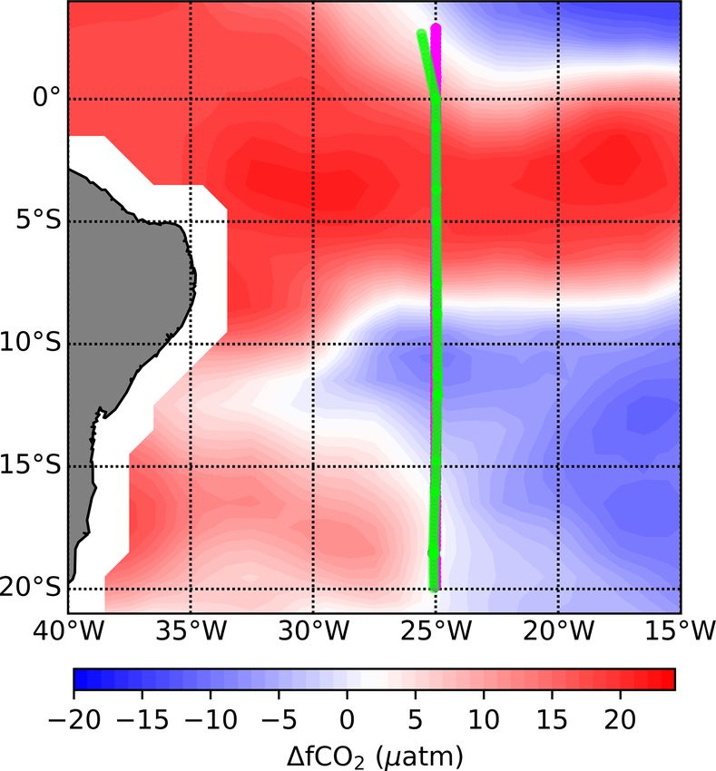
8090                                      Y. Dong et al.: Uncertainties in eddy covariance air–sea CO2 flux measurements

sured by a fast-response gas analyser, and the vertical wind      tuations from the sampled air. The simplest approach is to
velocity w (in m s−1 ) is often measured by a sonic anemome-      combine a closed-path gas analyser with a physical dryer to
ter. The prime denotes the fluctuations from the mean, while      eliminate most of the water vapour fluctuation (Miller et al.,
the overbar indicates time average. Equation (2) does not rely    2010; Blomquist et al., 2014; Landwehr et al., 2014; Yang
on 1f CO2 measurements, nor empirical parameters and as-          et al., 2016; Nilsson et al., 2018). The tuneable-diode-laser-
sumptions of the gas properties (Wanninkhof, 2014). EC flux       based cavity ring-down spectrometer (CRDS) made by Pi-
measurements can therefore be considered useful as an inde-       carro Inc. (Santa Clara, California, USA) is the most precise
pendent reference for bulk air–sea CO2 flux estimates. Fur-       closed-path analyser currently available (Blomquist et al.,
thermore, the typical temporal and spatial scales of EC flux      2014). The closed-path infrared gas analyser LI-7200 (LI-
measurements are ca. hourly and 1–10 km2 . These scales are       COR Biosciences, Lincoln, Nebraska, USA) is another pop-
much smaller than the temporal and spatial scales of alterna-     ular choice.
tive techniques for measuring gas transfer, e.g. by dual tracer      The advancements in instrumentation and in motion cor-
methods (daily and 1000 km2 ) (Nightingale et al., 2000; Ho       rection methods have significantly improved the quality of
et al., 2006). EC measurements are thus potentially better        air–sea EC CO2 flux observations, but, despite these changes,
suited to capture variations in gas exchange due to small-        the flux uncertainties have not been well quantified. The aims
scale processes at the air–sea interface (Garbe et al., 2014).    of this study are to (1) analyse uncertainties in EC air–sea
   The EC CO2 flux method has developed and improved              CO2 flux measurements; (2) propose practical methods to re-
over time. Before 1990, EC was successfully used to mea-          duce the systematic and random flux uncertainty; and (3) in-
sure air–sea momentum and heat fluxes. EC air–sea CO2             vestigate how the EC flux uncertainty influences our ability
flux measurements made during those times were unreason-          to estimate and parameterise K660 .
ably high (Jones and Smith, 1977; Wesely et al., 1982; Smith
and Jones, 1985; Broecker et al., 1986). After 1990, with
the development of the infrared gas analyser, EC became           2     Experiment and methods
routinely used for terrestrial carbon cycle research (Baldoc-
chi et al., 2001). Development of the EC method was ac-           2.1    Instrumental setup
companied by improvements in the flux uncertainty analysis,
which was generally based on momentum, heat and land–             The basic information of four cruises is summarised in Ta-
atmosphere gas flux measurements (Lenschow and Kris-              ble 1. Appendix A shows the four cruise tracks (Figs. A1
tensen, 1985; Businger, 1986; Lenschow et al., 1994; Wien-        and A2). Data from the Atlantic cruises (AMT28 and
hold et al., 1995; Mahrt, 1998; Finkelstein and Sims, 2001;       AMT29) are limited to 3◦ N–20◦ S in order to focus specifi-
Loescher et al., 2006; Rannik et al., 2009, 2016; Billesbach,     cally on the performance of two different gas analysers in the
2011; Mauder et al., 2013; Langford et al., 2015; Post et al.,    same region with low flux signal (tropical zone).
2015).                                                               The CO2 flux and data logging systems installed on the
   In the late 1990s, the advancement in motion correction of     JCR and Discovery were operated autonomously. The EC
wind measurements (Edson et al., 1998; Yelland et al., 1998)      systems were approximately 20 m a.m.s.l. on both ships (at
facilitated ship-based EC CO2 flux measurements from a            the top of the foremasts; Fig. 1) to minimise flow distor-
moving platform (McGillis et al., 2001; 2004). After 2000,        tion and exposure to sea spray. Computational fluid dynamics
a commercial open-path infrared gas analyser LI-7500 (Li-         (CFD) simulation indicates that the airflow distortion at the
COR Inc. USA) became widely used for air–sea CO2 flux             top of the JCR foremast is small (∼ 1 % of the free stream
measurements (Weiss et al., 2007; Kondo and Tsukamoto,            wind speed when the ship is head to wind; Moat and Yel-
2007; Prytherch et al., 2010; Edson et al., 2011; Else et al.,    land, 2015). The hull structure of RRS Discovery is nearly
2011; Lauvset et al., 2011). The LI-7500 generated ex-            identical to that of RRS James Cook. CFD simulation of the
tremely large and highly variable CO2 fluxes in comparison        James Cook indicates that the airflow at the top foremast is
to expected fluxes (Kondo and Tsukamoto, 2007; Prytherch          distorted by ∼ 2 % for bow-on flows (Moat et al., 2006). The
et al., 2010; Edson et al., 2011; Else et al., 2011; Lauvset      deflection of the streamline from horizontal and effects on
et al., 2011). This problem is generally considered to be an      the vertical wind component is accounted for by the double
artefact caused by water vapour cross-sensitivity (Kohsiek,       rotation (motion correction processes; see Sect. 2.2) prior to
2000; Prytherch et al., 2010; Edson et al., 2011; Landwehr        the EC flux calculation for both ships.
et al., 2014). Mathematical corrections proposed to address          The EC system on the JCR consists of a three-dimensional
this artefact (Edson et al., 2011; Prytherch et al., 2010) were   sonic anemometer (Metek Inc., Sonic-3 Scientific), a mo-
later shown to be unsatisfactory (Else et al., 2011; Ikawa        tion sensor (initially Systron Donner Motionpak II, which
et al., 2013; Blomquist et al., 2014; Tsukamoto et al., 2014)     compared favourably with and was then replaced by a Life
or incorrect (Landwehr et al., 2014).                             Performance-Research LPMS-RS232AL2 in April 2019),
   The most reliable method for measuring EC air–sea CO2          and a Picarro G2311-f gas analyser. All instruments sam-
fluxes involves the physical removal of water vapour fluc-        pled at a frequency of 10 Hz or greater, and the data were

Atmos. Chem. Phys., 21, 8089–8110, 2021                                            https://doi.org/10.5194/acp-21-8089-2021

Y. Dong et al.: Uncertainties in eddy covariance air–sea CO2 flux measurements                                                           8091

Table 1. Basic information for all four cruises on the RRS James Clark Ross (JCR) and RRS Discovery that measured air–sea EC CO2
fluxes.

    Cruise             JR18006                         JR18007                        AMT28                       AMT29
    Data period        30 Jun–1 Aug 2019               5 Aug–29 Sep 2019              9–16 Oct 2018               4–11 Nov 2019
    Visited region     Arctic Ocean (Barents Sea)      Arctic Ocean (Fram Strait)     Tropical Atlantic Ocean     Tropical Atlantic Ocean
    Research vessel    JCR                             JCR                            JCR                         Discovery
    Gas analyser       Picarro G2311-f                 Picarro G2311-f                Picarro G2311-f             LI-7200

Figure 1. EC system (upper panel) and a diagram of the system setup (bottom panel). EC instruments: (1) sonic anemometer, (2) motion
sensor, (3) air sample inlet for gas analyser, (4) data logger/gas analyser. Arctic and Atlantic data from 2018 were collected on the RRS James
Clark Ross (JCR; upper right) using a Picarro G2311-f, and Atlantic data from 2019 were collected using a LI-7200 on the RRS Discovery
(upper left).

logged at 10 Hz with a data logger (CR6, Campbell Scien-                  within the enclosed staircase, directly underneath the meteo-
tific, Inc.), similar to the setup by Butterworth and Miller              rological platform and close to the inlet (inlet length 7.5 m,
(2016). Air is pulled through a long tube (30 m, inner diame-             inner diameter 0.95 cm, Reynolds number 1042). A single
ter 0.95 cm, Reynolds number 5957) with a dry vane pump at                pump (Gast 1023) was sufficient to pull air through a parti-
a flow rate of ∼ 40 L min−1 (Gast 1023 series). The Picarro               cle filter (Swagelok 2 µm), a dryer (Nafion PD-200T-24M),
gas analyser subsamples from this tube through a particle fil-            and the LI-7200 at a flow of ∼ 7 L min−1 . There was no N2
ter (Swagelok 2 µm) and a dryer (Nafion PD-200T-24M) at                   puff system setup on Discovery, but equivalent lab tests con-
a flow of ∼ 5 L min−1 (Fig. 1). The dryer is set up in the                firmed that the delay time was less than on the JCR because
“re-flux” configuration and uses the lower pressure Picarro               of the shorter inlet line. The dryer on the Discovery is set
exhaust to dry the sample air. This method removes ∼ 80 %                 up in the same re-flux configuration as the JCR and uses the
of the water vapour and essentially all of the humidity fluc-             lower pressure at the LI-7200 exhaust (limited by an addi-
tuations (Yang et al., 2016). The Picarro internal calculation            tional 0.08 cm diameter critical orifice) to dry the sample air.
accounts for the detected residual water vapour and yields a              This setup removes ∼ 60 %–70 % of the water vapour and es-
dry CO2 mixing ratio that is used in the flux calculations. A             sentially all of the humidity fluctuations. The dry CO2 mix-
valve controlled by the Picarro instrument injects a “puff” of            ing ratio, computed by accounting for the LI-7200 temper-
nitrogen (N2 ) into the tip of the inlet tube for 30 s every 6 h.         ature, pressure, and residual water vapour measurements, is
This enables estimates of the time delay and high-frequency               used in the flux calculations.
signal attenuation (Sect. 2.2).
    The EC system on RRS Discovery consists of a Gill R3-50               2.2   Flux processing
sonic anemometer, a LPMS motion sensor package, and a LI-
7200 gas analyser. The LI-7200 gas analyser was mounted                   The EC air–sea CO2 flux calculation steps using the raw data
                                                                          are outlined with a flow chart (Fig. 2) and detailed below. The

https://doi.org/10.5194/acp-21-8089-2021                                                    Atmos. Chem. Phys., 21, 8089–8110, 2021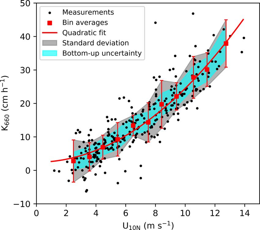
8092                                          Y. Dong et al.: Uncertainties in eddy covariance air–sea CO2 flux measurements

Figure 2. Flow chart of EC data processing. The raw high-frequency (10 Hz) wind and CO2 data were initially processed separately and then
combined to calculate fluxes. CO2 fluxes were filtered by a series of data quality control criteria. The 20 min flux intervals were averaged to
longer timescales (hourly or more). The data processing is detailed in the text.

raw high-frequency wind and CO2 data are processed first,                 ship, yielding the vertical wind velocity (w) required in
yielding fluxes in 20 min averaging time interval and related             Eq. (2). Inspection of frequency spectra showed that the spec-
statistics. These statistics are then used for quality control of         tral peak at the ship motion frequencies (approximately 0.1–
the fluxes. Further averaging of the quality-controlled 20 min            0.3 Hz) had disappeared after the motion correction (Fig. S1
fluxes to hourly or longer timescales is then used to reduce              in the Supplement). This indicates that the majority of ship
random error (Sect. 4.1). Linear detrending was used to iden-             motion had been removed from the measured wind speed.
tify the turbulent fluctuations (i.e. w0 and c0 ) throughout the          The last step in the wind data processing was the calculation
analyses.                                                                 of 20 min average friction velocity, sensible heat flux, and
   To correct the wind data for ship motion, we first generated           other key variables used for data quality control (Table S1 in
hourly data files containing the measurements from the sonic              the Supplement).
anemometer (three-dimensional wind speed components: u,                      The CO2 data were de-spiked (by removing val-
v, and w and sonic temperature Ts ), motion sensor (three axis            ues > 4 SDs from the median). The Picarro CO2 mixing ratio
accelerations: accel_x, accel_y, accel_z; and rotation angles:            was further decorrelated against analyser cell pressure and
rot_x, rot_y, rot_z), ship heading over ground (HDG; from                 temperature to remove CO2 variations due to the ship’s mo-
the gyro compass), and ship speed over ground (SOG; from                  tion. The LI-7200 CO2 mixing ratio was further decorrelated
Global Position System). Spikes larger than 4 standard devia-             against the LI-7200 H2 O mixing ratio and temperature to re-
tions (SDs) from the median were removed. Secondly, a com-                move residual air density fluctuations, following Landwehr
plementary filtering method using Euler angles (see Edson                 et al. (2018). CO2 data were also decorrelated against the
et al., 1998) was applied to the hourly data files to remove ap-          ship’s heave and accelerations because these can produce
parent winds generated by the ship movements. The motion-                 spurious CO2 variability (Miller et al., 2010; Blomquist et al.,
corrected winds were further decorrelated against ship mo-                2014).
tion to remove any residual motion-sensitivity (Miller et al.,               A lag between CO2 data acquisition and the wind data is
2010; Yang et al., 2013). The motion-corrected winds were                 created because of the time taken for sample air to travel
double-rotated to account for the wind streamline over the                through the inlet tube. On the JCR, we use the puff system

Atmos. Chem. Phys., 21, 8089–8110, 2021                                                      https://doi.org/10.5194/acp-21-8089-2021
Y. Dong et al.: Uncertainties in eddy covariance air–sea CO2 flux measurements                                               8093

where the lag time is the time difference between the N2            (Sect. 2.3.3). Errors due to insufficient sampling and in-
puff start (when the on/off valve is switched) and the time         strument noise are generally considered most important in
when the diluted signal is sensed by the gas analyser. The          EC flux measurements (Lenschow and Kristensen, 1985;
lag time can also be estimated by the maximum covariance            Businger, 1986; Mauder et al., 2013; Rannik et al., 2016).
method, calculated by shifting the time base of the CO2 sig-           Sampling error is an inherent issue for EC flux measure-
nal and finding the shift that achieves maximum covariance          ments and is typically the main source of the CO2 flux un-
between the vertical wind velocity (w) signal and the shifted       certainty (Mauder et al., 2013). The sampling error is caused
CO2 signal. The lag times estimated by the maximum covari-          by the difference between the ensemble average and the time
ance method agree well with the estimates of the puff proce-        average. The calculation of EC flux (Eq. 2) requires the sepa-
dure (Fig. S2 in the Supplement). These estimates indicate a        ration between the mean and fluctuating components, which
lag time of 3.3–3.4 s for the Arctic cruises and 3.3 s for cruise   can be represented fully for CO2 mixing ratio c as
AMT28 on the JCR. The lag time on Discovery (AMT29) es-
timated by the maximum covariance method was 2.6 s, con-            c(x, t) = c(x, t) + c0 (x, t).                             (4)
sistent with laboratory test results prior to the cruise.
   The inlet tube, particle filter, and dryer cause high-              The mean component c represents ensemble average over
frequency CO2 flux signal attenuation. The N2 puff was also         time (t) and space (x) and does not contribute to the flux.
used to assess the response time by considering the e-folding       The time average of a stationary turbulent signal and space
time in the CO2 signal change (similar approaches have been         average of a homogenous turbulent signal theoretically con-
used by Bariteau et al., 2010; Blomquist et al., 2014, Bell         verge on the ensemble average when the averaging time ap-
et al., 2015). The response time is 0.35 s for the EC system        proaches infinity, i.e. T → ∞ (Wyngaard, 2010). In prac-
on JCR and 0.25 s for the EC system on Discovery (estimated         tice, Reynolds averaging over a much shorter time inter-
in the laboratory prior to cruise). These response times were       val (10 min to an hour) is typically used for EC flux mea-
combined with the relative wind speed-dependent, theoreti-          surements from a fixed point or from a slow-moving plat-
cal shapes of the cospectra (Kaimal et al., 1972) to estimate       form such as a ship. This is because the atmospheric bound-
the percentage flux loss due to the inlet attenuation (Yang         ary layer is only quasi-stationary for a few hours. Non-
et al., 2013). The mean attenuation percentage is less than         stationarity (e.g. diurnal variability and synoptic conditions)
10 %, with a relative wind speed dependence (Fig. S3 in the         is an inherent property of the atmospheric boundary layer
Supplement). The attenuation percentage value was applied           (Wyngaard, 2010). EC flux observations thus inevitably con-
to the computed flux to compensate for the flux loss due            tain some random error due to insufficient sampling time, and
to the high-frequency signal attenuation. Finally, horizontal       this error is greater at shorter averaging times.
CO2 fluxes and other statistics such as CO2 range and CO2              Random error due to instrument noise comes mainly from
trend were computed for quality control purposes (Table S1,         the white noise of the gas analyser, as the noise from the
Supplement).                                                        sonic anemometer is relatively unimportant (Blomquist et al.,
   The computed 20 min fluxes were filtered for non-ideal           2010; Fairall et al., 2000; Mauder et al., 2013). Blomquist
ship manoeuvres or violations of the homogeneity/stationary         et al. (2014) show “pink” noise with a weak spectral slope for
requirement of EC (see Supplement for the quality control           their CRDS gas analyser (G1301-f), but the gas analysers on
criteria).                                                          JCR (G2311-f) and Discovery (LI-7200) demonstrate white
                                                                    noise with a constant variance at high frequency (Fig. B2,
2.3     Uncertainty analysis methods                                Appendix B).

2.3.1    Uncertainty components                                     2.3.2   Systematic error

Uncertainty contains two components: systematic error               Table 2 details the measures taken during instrument setup
(δFS ) and random error (δFR ). According to propagation of         and data processing that help eliminate most sources of sys-
uncertainty theory (JCGM, 2008), the total uncertainty in EC        tematic error in EC CO2 fluxes.
CO2 fluxes (from random and systematic errors) can be ex-              In addition to bias sources related to the instrument setup
pressed as                                                          (Table 2), insufficient sampling time (an inherent issue of EC
                                                                    fluxes) may also generate a systematic error. We use a the-
                                                                    oretical method to estimate this systematic error in EC CO2
        q
δF =        δFR2 + δFS2 .                                    (3)    flux (Lenschow et al., 1994):
   Systematic errors (Sect. 2.3.2) will cause bias in the flux.                      √
                                                                                        τw τc
They thus should be eliminated/minimised with the appro-            |δFS | ≤ 2σw σca          ,                                 (5)
                                                                                        T
priate system setup and, if needed, effective numerical cor-
rections. Random error results in imprecision (but not bias)        where σw (m s−1 ) and σca (ppm) are the standard deviations
and can be reduced by averaging repeated measurements               of the vertical wind velocity and the CO2 mixing ratio due to

https://doi.org/10.5194/acp-21-8089-2021                                              Atmos. Chem. Phys., 21, 8089–8110, 2021
8094                                         Y. Dong et al.: Uncertainties in eddy covariance air–sea CO2 flux measurements

Table 2. Potential sources of bias in our EC air–sea CO2 flux measurements and the methods used to minimise them.

   Potential source               Methods used to minimise the bias                                                         Flux
   of bias                                                                                                                  uncertainty
   δFS,1                          Closed-path gas analyser with a dryer removes essentially all of the water vapour         Negligible
   Water vapour                   fluctuation (Blomquist et al., 2014; Yang et al., 2016). The residual H2 O signal is
   cross-sensitivity              measured by the gas analyser and used in the calculation of the dry CO2 mixing
                                  ratio, which removes water cross-sensitivity.
   δFS,2                          Flux uncertainty from an earlier version of the motion correction procedure (less         ≤6%
   Ship motion                    rigorous than the one used by ourselves) is estimated to be 10 %–20 % (Edson
                                  et al., 1998). The more recently adopted decorrelation of vertical winds and CO2
                                  against platform motion (Miller et al., 2010; Yang et al., 2013) reduces this uncer-
                                  tainty. Flügge et al. (2016) compare EC momentum fluxes measured from a moving
                                  platform (buoy) with fluxes measured from a nearby fixed tower. Flux estimates
                                  from these two platforms agree well (relative flux bias due to the motion correction
                                  ≤ 6 %).
   δFS,3                          The EC flux system is deployed as far forward and as high as possible on the ship         Negligible
   Airflow distortion             (top of the foremast), which minimises the impacts of flow distortion. Subsequent
                                  distortion correction using the CFD simulation (Moat et al., 2006; Moat and Yel-
                                  land, 2015) along with a relative wind direction restriction further reduces the im-
                                  pact of flow distortion on the fluxes. Measured EC friction velocities and friction ve-
                                  locities from the COARE3.5 model (Edson et al., 2013) agree well (e.g. R 2 = 0.95,
                                  slope = 0.97) for data collected during cruise JR18006. Good comparison between
                                  observed and COARE3.5 friction velocity estimates indicates that we have fully
                                  accounted for flow distortion effects.
   δFS,4                          High-frequency flux signal attenuation (in the inlet tube, particle filter, and dryer)    < 2 % for vast
   Inlet effects (high-           is evaluated by the CO2 signal response to a puff of N2 gas. Flux attenuation             majority of the
   frequency flux attenuation     is calculated from the “inlet puff” response and applied as a correction (< 10 %;         cruises
   and CO2 sampling delay)        see Sect. 2.2). The uncertainty in the attenuation correction is about 1 % for un-
                                  stable/neutral atmospheric conditions, which is generally the case over the ocean
                                  (e.g. 93 % of the time for the Atlantic cruises, 80 % of the time for the Arctic
                                  cruises). During stable conditions, the attenuation correction is larger (Landwehr
                                  et al., 2018), and the uncertainty is also greater (∼ 20 %).
                                  The lag time adjustment prior to the flux calculation aligns the CO2 and wind sig-
                                  nals. Two methods are used to estimate the optimal lag time: puff injection and
                                  maximum covariance. The two lag estimates are in good agreement (Sect. 2.2).
                                  Random adjustment of ± 0.2 s (1σ of the puff test result) to the optimal lag time
                                  impacts the CO2 flux by < 1 %.
   δFS,5                          The CO2 inlet is ∼ 70 cm directly below the centre volume of the sonic anemome-           Negligible
   Spatial separation between     ter. This distance is small relative to the size of the dominant flux-carrying eddies
   the sonic anemometer and       encountered by the EC measurement system height above sea level. The excellent
   the gas inlet                  agreement between the lag time determined by the puff system and by the optimal
                                  covariance method further confirms that the distance between the CO2 inlet and
                                  anemometer is sufficiently small.
   δFS,6                          The potential flux bias resulting from instrument calibration (gas analyser,              ≤4%
   Imperfect calibration of the   anemometer and meteorological sensors required to calculate air density: air tem-
   sensors                        perature, relative humidity and pressure) is up to 4 % for the JCR setup. The
                                  largest instrument calibration uncertainty derives from the wind sensor accuracy
                                  (± 0.15 m s−1 at 4 m s−1 winds according to the Metek uSonic instrument specifi-
                                  cation). This bias is even lower (< 2 %) for the Discovery setup because the Gill R3
                                  sonic anemometer is more accurate.
   Propagated bias                Estimated from the individual bias estimates above (δFS,1 , δFS,2 , etc.) using δFS =     < 7.5 %
                                  s
                                    n
                                    P    2
                                       δFS,n
                                    1

Atmos. Chem. Phys., 21, 8089–8110, 2021                                                       https://doi.org/10.5194/acp-21-8089-2021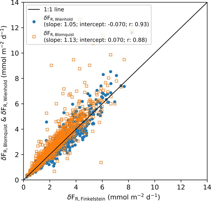
Y. Dong et al.: Uncertainties in eddy covariance air–sea CO2 flux measurements                                              8095

atmospheric processes, respectively. T is the averaging time          in the brackets represents the auto-covariance compo-
interval (s), and τw and τc are integral timescales (s) for ver-      nent, and the second term is the cross-covariance com-
tical wind velocity and CO2 signal, respectively. The defi-           ponent. rww and rcc are the auto-covariance functions
nition and estimation of the integral timescale are shown in          for vertical wind velocity (w) and CO2 mixing ratio (c),
Appendix B. The sign of δFS could be positive or negative             respectively. rwc and rcw are the cross-covariance func-
(i.e. under- or overestimation) because of the poor statistics        tions for w and c. Here rwc represents shifting w data
in capturing low-frequency eddies within the flux averaging           relative to CO2 data, while rcw represents shifting CO2
period (Lenschow et al., 1993). The mean hourly relative              data relative to w data.
systematic error due to insufficient sampling time for four
cruises estimated by Eq. (5) is < 5 %. According to propaga-       C. Blomquist et al. (2010) attributed the sources of CO2
tion of uncertainty theory√(JCGM, 2008), the total systematic         variance σc2 to atmospheric processes (σc2a ) and white
error is less than 9 % (= 7.5 %2 + 5 %2 ).                            noise (σc2n ). The sources of variance are considered to be
                                                                      independent of each other, and the sonic anemometer is
2.3.3   Random error                                                  assumed to be relatively noise-free. According to prop-
                                                                      agation of uncertainty theory (JCGM, 2008), the total
Five approaches used to estimate the total random error (A–           random flux error can be defined as
C) and the random error component due to instrument noise                                 aσw                1/2
(C–E) in EC CO2 fluxes are discussed below. The random                δFR,Blomquist ≤ √ σc2a τwc + σc2n τcn        ,          (7)
                                                                                             T
error assessments are empirical (A and D) or theoretical (B,
                                                                                                            √
C, and E).                                                            where the constant a varies from 2 to 2, depending
                                                                      on the relationship between the covariance of the two
 A. An empirical approach to estimate total random er-                variables (w and CO2 ) and the product of their auto-
    ror involves shifting the w data relative to the CO2              correlations (Lenschow and Kristensen, 1985). Here,
    data (or vice versa) by a large, unrealistic time shift           τwc is equal to the shorter of τw and τc , which is typ-
    and then computing the “null fluxes” from the time-               ically τw (Blomquist et al., 2010), and τcn is the inte-
    desynchronized CO2 and w time series (Rannik et al.,              gral timescale of white noise in the CO2 signal. The
    2016). The shift removes any real correlation between             CO2 variance due to atmospheric processes (σc2a ) in-
    CO2 and w due to vertical exchange. The standard de-              cludes two components: variance due to vertical flux
    viation of the resultant null fluxes represents the random        (i.e. air–sea CO2 flux), σc2av , and variance due to other
    flux uncertainty (Wienhold et al., 1995). We applied
                                                                      atmospheric processes, σc2ao (Fairall et al., 2000). The
    a series of time shifts of ∼ 20–60 · τw (i.e. using time
    shifts ranging from −300 to −100 and 100 to 300 s;                variance in CO2 due to vertical flux (σc2av ) depends
    Rannik et al., 2016). This empirical estimation of to-            on atmospheric stability. σc2av can be estimated with
    tal random flux uncertainty will hereafter be referred to         Monin–Obukhov similarity theory (Blomquist et al.,
    as δFR,Wienhold .                                                 2010, 2014; Fairall et al., 2000):
                                                                              "                  #2
 B. Lenschow and Kristensen (1985) derived a rigorous                   2         w 0 c0
                                                                      σcav = 3           fc (z/L) ,                           (8)
    theoretical equation for total random error estimation,                        u∗
    which contains both the auto-covariance and cross-
    covariance functions. The theoretical equation has been           where u∗ is the friction velocity (m s−1 ), and the similar-
    numerically approximated by Finkelstein and Sims                  ity function (fc ) depends on the stability parameter z/L,
    (2001):                                                           where z is the observational height (m), and L is the
                                                                      Obukhov length (m). The expression of fc can be found
                        " Xm
                        1                                             in Blomquist et al. (2010).
     δFR,Finkelstein =          rww (p)rcc (p)
                        n p= −m                                       Equation (7) can be used to assess the random error
                          m
                                            # 1/2                    due to instrument noise by setting σc2a = 0, referred to
                       +
                          X
                             rwc (p)rcw (p)        ,        (6)       hereafter as δFRN,Blomquist . We use the CO2 variance
                        p= −m                                         spectra to directly estimate the white noise term σc2n τcn
                                                                      in Eq. (7). The variance is fairly constant at high fre-
     where n is the number of data points within an averag-           quency (1–5 Hz; Fig. B2, Appendix B), which is often
     ing time interval, and p is the number of shifting points.       referred to as band-limited white noise. The relation-
     The maximum shifting point m can be chosen subjec-               ship between σc2n τcn and the band-limited noise spectral
     tively ( < n). We found that the random error for m be-          value ϕcn is expressed in Blomquist et al. (2010) as
     tween 1000 and 2000 data points was similar, so for this                      ϕc n
     study we use m = 1500 (150 s shift time). The first term         σc2n τcn =        .                                     (9)
                                                                                    4

https://doi.org/10.5194/acp-21-8089-2021                                             Atmos. Chem. Phys., 21, 8089–8110, 2021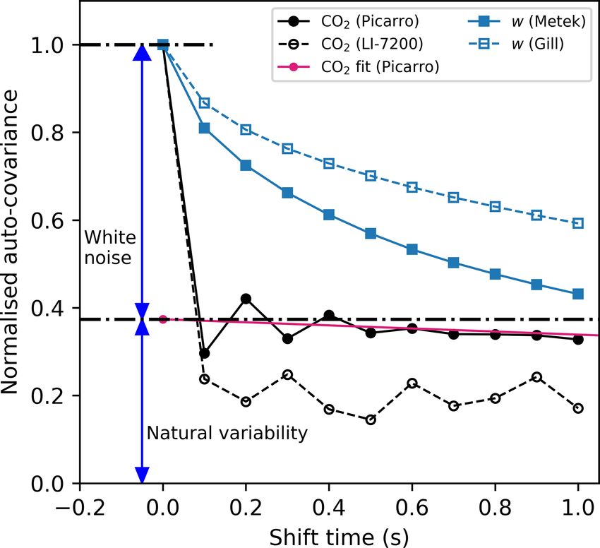
8096                                        Y. Dong et al.: Uncertainties in eddy covariance air–sea CO2 flux measurements

    D. Billesbach (2011) developed an empirical method to es-
       timate the random error due to instrument noise alone
       (referred to as 1FRN,Billesbach ). This involves random
       shuffling of the CO2 time series within an averaging in-
       terval and then calculating the covariance of w and CO2 .
       The correlation between w and CO2 is minimised by the
       shuffling, and any remaining correlation between w and
       CO2 is due to the unintentional correlations contributed
       by instrument noise.
    E. Mauder et al. (2013) describe another theoretical ap-
       proach to estimate the random flux error due to instru-
       ment noise:
                      σw σc
       δFRN,Mauder = √ n .                               (10)
                         n
                                                                    Figure 3. Mean normalised auto-covariance functions of CO2 and
       White noise correlates with itself but is uncorrelated       vertical wind velocity (w) by four different instruments. The ma-
       with atmospheric turbulence. Thus, the white-noise-          genta line represents a fit to the noise-free auto-covariance function
       induced CO2 variance (σcn ) only contributes to the total    of CO2 (measured by Picarro) extrapolated back to a zero time shift.
       variance. The value of σcn can be estimated from the         An example of the white noise and natural variability contributions
                                                                    to the total CO2 (measured by Picarro) variance is indicated by two
       difference between the zero-shift auto-covariance value
                                                                    blue arrows. The sharp decrease of the CO2 auto-covariance be-
       (CO2 variance σc2 ) and the noise-free variance extrapo-     tween the zero shift and the initial 0.1 s shift corresponds to the large
       lated to a time shift of zero (Lenschow et al., 2000):       contribution of white noise from the gas analysers. The LI-7200 is
                                                                    the noisier instrument. The noise contributions from the anemome-
       σc2n = σc2 − σ 2 (t → 0),                            (11)    ter are relatively small (< 10 %).

       where σ 2 (t → 0) represents the extrapolation of auto-
       covariance to a zero shift, which is considered equal to     noise (δFRN,Mauder ) is about 3 times higher during AMT29
       variance due to atmospheric processes (σc2a ). Figure 3      using LI-7200 than during AMT28 using Picarro G2311-f
       shows the normalised auto-covariance function curves         (Fig. 4b; Fig. D1, Appendix D). The similar total random un-
       of w and CO2 as measured by the Picarro G2311-f and          certainty in the AMT28 and AMT29 fluxes shows that both
       the LI-7200. There is a sharp decrease in the CO2 auto-      gas analysers are equally suitable for air–sea EC CO2 flux
       covariance when shifting from 0 s shift to 0.1 s shift for   measurements. The variance budgets of atmospheric CO2
       both the Picarro G2311-f and LI-7200 gas analyser. The       mixing ratio (used to estimate random flux uncertainty; see
       same sharp decrease is not seen in the vertical wind ve-     Sect. 3.1) are shown in Fig. 4c. Total variance in CO2 mix-
       locity (w) auto-covariance. The relative difference in the   ing ratio is dominated by instrument noise on both cruises.
       change in normalised auto-covariance shows that white        CO2 mixing ratio variance (total and instrument noise) was
       noise makes a much larger relative contribution to the       substantially higher during AMT29.
       CO2 variance than to the vertical wind velocity vari-
       ance.                                                        3.1   Random uncertainty

                                                                    Theoretical derivation of flux uncertainty (δFRN,Blomquist ,
                                                                    Eq. 7) requires knowledge of the contributions to CO2 mix-
3     Results
                                                                    ing ratio variance. Total CO2 variance is made up of in-
Measurements from AMT28 and AMT29 set the scene for                 strument noise (σc2n ) and atmospheric processes (σc2a ). At-
our uncertainty analysis. These two Atlantic cruises transited      mospheric processes include vertical flux (σc2av ) and other
across the same tropical region (Fig. A2, Appendix A) in Oc-        atmospheric processes (σc2ao ). The variance budgets of CO2
tober 2018 and September 2019 with different eddy covari-           mixing ratio for the four cruises are listed in Table 3. At-
ance systems (Sect. 2.1). AMT28 and AMT29 show broadly              mospheric processes contribute a larger CO2 variance in the
similar latitudinal patterns (Fig. 4a). An obvious question of      Arctic (where flux magnitudes are greater) compared to the
interest is whether the measured fluxes were the same for           Atlantic. Vertical flux accounts for ∼ 10 % of the variance in
the 2 years. To answer this question, the measurement uncer-        CO2 mixing ratio in the Arctic and ∼ 1 % of the CO2 vari-
tainties must be quantified. The total random uncertainties in      ance in the Atlantic. Previous results demonstrate that hori-
CO2 flux (δFR,Finkelstein ) are comparable for the two cruises,     zontal transport is a major source of σc2ao for long-lived green-
even though the random error component due to instrument            house gases (Blomquist et al., 2012). Small changes in CO2

Atmos. Chem. Phys., 21, 8089–8110, 2021                                                 https://doi.org/10.5194/acp-21-8089-2021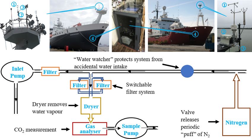
Y. Dong et al.: Uncertainties in eddy covariance air–sea CO2 flux measurements 8097
Figure 4. (a) Air–sea CO2 fluxes (hourly and 6 h averages), (b) random uncertainty in flux (total and due to instrument noise only), and
(c) variance in CO2 mixing ratio (total and due to instrument noise only) for two Atlantic cruises.
Table 3. Variance in the CO2 mixing ratio estimated using Eqs. (8) and (11) for the Arctic (JR18006/7, Picarro G2311-f) and Atlantic cruises
(AMT28, Picarro G2311-f; AMT29, LI-7200). Total CO2 variance (σc2 ) consists of white noise (σc2n ) and atmospheric processes (σc2a ). The
latter can be further broken down to the CO2 variance due to vertical flux (σc2av ) and due to other processes (σc2ao ).
CO2 variance (× 10−3 ppm2 ) JR18006 JR18007 AMT28 AMT29
Total, σc2 9.9 8.6 3.6 13.9
Due to instrument white noise, σc2n 5.8 5.4 2.0 12.6
Due to atmospheric processes, σc2a 4.1 3.3 1.6 1.3
– Due to vertical flux, σc2av 1.3 0.8 0.03 0.08
– Due to other atmospheric processes, σc2ao 2.8 2.5 1.6 1.2
mixing ratio transported horizontally can yield variance that We used three methods to estimate the total random un-
greatly exceeds the variance from vertical flux. certainty (δFR ; Methods A–C, Sect. 2.3.3) in the hourly aver-
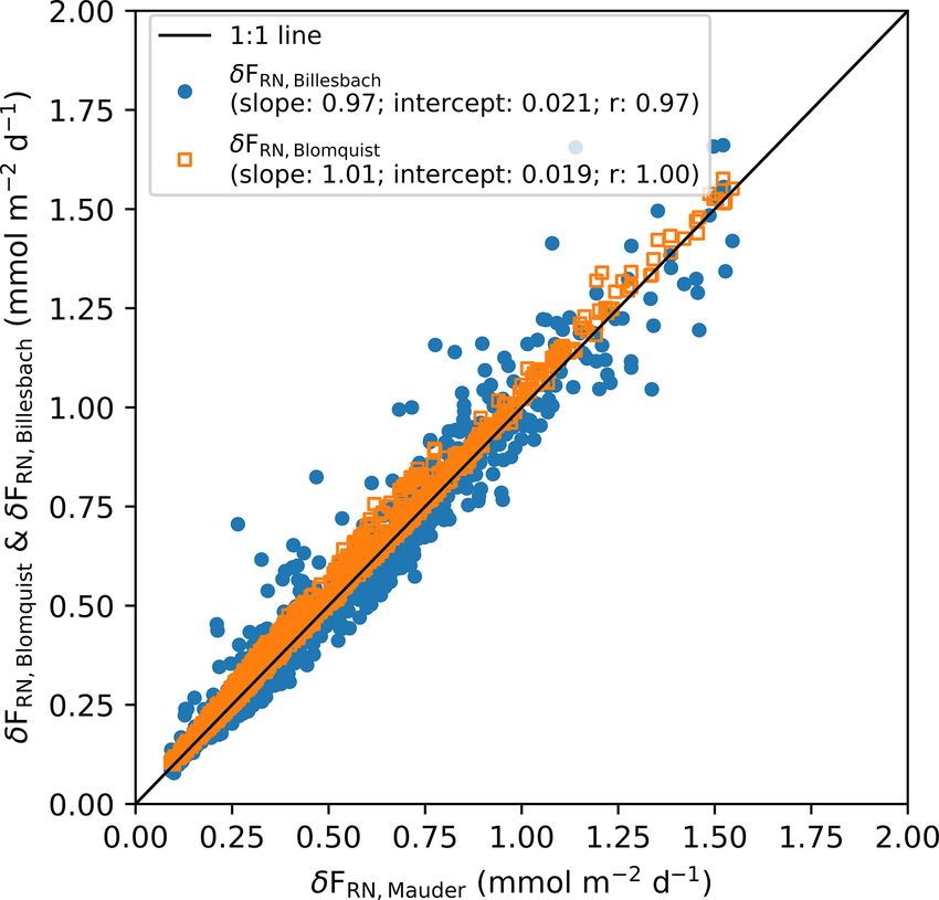
Three quasi-independent methods were used to estimate aged air–sea CO2 fluxes. There is good agreement among the
random uncertainty in EC air–sea CO2 fluxes caused by three estimates (r > 0.88; Fig.√ C1, Appendix C). Again, the
instrument noise (δFRN ; Methods C–E, Sect. 2.3.3). Good constant in Eq. (7) (a) is set to 2, as informed by the instru-
agreement was found √ between all three estimates (Fig. C2, ment noise uncertainty analysis above. We use δFR,Finkelstein
Appendix C) when 2 is used as the constant in Eq. (7) (a). (Eq. 6) to estimate the total random flux uncertainty here-
The 1FRN,Billesbach estimates have more scatter and are after. Our decision is based on δFR,Finkelstein not requiring
slightly higher than the theoretical results, possibly because the integral timescale (unlike δFR,Blomquist ) and showing less
the random shuffling of data fails to fully exclude the con- scatter than δFR,Wienhold .
tribution from atmospheric turbulence (Rannik et al., 2016). Figure 5 shows the different relative contributions to the
For the remainder of this study, we use the δFRN,Mauder random flux uncertainty for the Arctic cruises (hourly aver-
method to estimate δFRN . age). Here the uncertainty is normalised by the flux magni-
tude and then averaged into flux magnitude bins. When the
https://doi.org/10.5194/acp-21-8089-2021 Atmos. Chem. Phys., 21, 8089–8110, 2021
8098                                          Y. Dong et al.: Uncertainties in eddy covariance air–sea CO2 flux measurements

Figure 5. Relative random uncertainty in hourly CO2 flux and its
                                                                       Figure 6. Comparison of relative random uncertainty in
contribution from noise, vertical flux, and other processes during
                                                                       hourly CO2 flux and relative standard deviation (RSTD;
two Arctic cruises. Relative random uncertainty data are binned into
                                                                       standard deviation/|flux mean|) of the EC CO2 flux from two Arc-
3 mmol m−2 d−1 flux magnitude bins (error bars represent 1 stan-
                                                                       tic cruises. These results are binned in 1 m s−1 wind speed bins.
dard deviation).

                                                                       flux from this region was 0.5 mmol m−2 d−1 , which is indis-
flux magnitude is sufficiently large (> 20 mmol m−2 d−1 ),             tinguishable from zero considering the random uncertainty.
the total relative random uncertainty in flux asymptotes to            This further confirms the minimal bias in our flux observa-
about 15 % and is driven by variance associated with both              tions.
vertical flux and other atmospheric processes. This estimate              Figure 6 shows a comparison between the relative un-
is similar to uncertainties in air–sea fluxes of other well re-        certainty and the relative standard deviation (RSTD) in the
solved (i.e. high signal-to-noise ratio) variables (Fairall et al.,    hourly CO2 flux for the two Arctic cruises. Results have
2000). At a lower flux magnitude, uncertainty due to atmo-             been binned into 1 m s−1 wind speed bins. Wind speed
spheric processes other than vertical flux dominates the total         was converted to 10 m neutral wind speed (U10N ) using the
random uncertainty. Uncertainty due to the white noise from            COARE3.5 model (Edson et al., 2013). The relative random
the Picarro G2311-f gas analyser is small.                             error decreases with increasing wind speed. This is partly be-
                                                                       cause the fluxes tend to be larger at higher wind speeds, and
3.2    Summary of systematic and random uncertainties                  so the signal-to-noise ratio in the flux is greater. In addition,
                                                                       at higher wind speeds, a greater number of high-frequency
The total uncertainty δF in the hourly average EC CO2 flux             turbulent eddies are sampled by the EC system, providing
(estimated using Eq. 3) ranges from 1.4 to 3.2 mmol m−2 d−1            better statistics of turbulent eddies and lower sampling error.
in the mean for the four cruises (Table 4). Our EC flux sys-              The RSTD of the flux is greater in magnitude than the
tem setup was optimal, and subsequent corrections have min-            estimated flux uncertainty because it also contains environ-
imised any bias to < 9 % (Sect. 2.3.2). Systematic error is            mental variability. The CO2 flux auto-covariance analysis
on average much lower than random error (Table 4). This                (Sect. 4.1) shows that random error in hourly flux explains
means the accuracy of the EC CO2 flux measurements is very             ∼ 20 % of the flux variance on average for the two Arctic
high, but the precision of hourly averaged EC CO2 air–sea              cruises. This implies that the remaining variability in the EC
flux measurements is relatively low. In Sect. 4.1, we discuss          flux (∼ 80 %) is due to natural phenomena (e.g. changes in
how the precision can be improved by averaging the observed            1f CO2 or wind speed). Similarly, substantial variability is
fluxes for longer.                                                     typical in EC-derived CO2 gas transfer velocity at a given
   The theoretical uncertainty estimates above can be com-             wind speed (e.g. Edson et al., 2011; Butterworth and Miller,
pared with a portion of the AMT28 cruise data (15–20◦ S,               2016). K660 is derived from (EC CO2 flux)/1f CO2 , and thus
∼ 25◦ W; Fig. 4), when the ship encountered sea surface                an understanding of EC flux uncertainty can help understand
CO2 fugacity close to equilibrium with the atmosphere (i.e.            and explain the variability in EC-derived gas transfer velocity
1f CO2 ∼ 0; Fig. A2, Appendix A). The data from this re-               estimates (Sect. 4.2).
gion are useful for assessing the random and systematic flux
uncertainties. The standard deviation of the EC CO2 flux dur-
ing cruise AMT28 when 1f CO2 ∼ 0 is 1.6 mmol m−2 d−1 ,
which compares well with the theoretical random flux uncer-
tainty in this region (1.4 mmol m−2 d−1 ). The mean EC CO2

Atmos. Chem. Phys., 21, 8089–8110, 2021                                                  https://doi.org/10.5194/acp-21-8089-2021
Y. Dong et al.: Uncertainties in eddy covariance air–sea CO2 flux measurements 8099
Table 4. Summary of hourly average EC CO2 fluxes and associated uncertainties in the mean for the four cruises (mmol m−2 d−1 ). Shown
are the mean CO2 flux magnitude (|F |, mmol m−2 d−1 ), upper limitation of the total uncertainty (δF ; Eq. 3), upper limitation of the absolute
systematic error (|δFS |; propagated from Table 2 and Eq. 5), and random error (δFR ; Eq. 6). The
q random error components are white noise
(δFRN ; Eq. 10), vertical flux (δFRV ; Eqs. 7 and 8), and other atmospheric processes (δFRO = δFR2 − δFRN
2 − δF 2 ). The total uncertainty
RV
is also expressed as a percentage of the mean flux magnitude (δF /|F | · 100 %).
Cruises JR18006 JR18007 AMT28 AMT29
|CO2 flux|, |F | 10.1 16.3 2.5 3.5
Total uncertainty, δF (δF /|F | · 100 %) 2.3 (23 %) 3.2 (20 %) 1.4 (58 %) 1.7 (49 %)
Systematic error, |δFS | 0.8 1.2 0.3 0.3
Total random error, δFR 2.2 2.9 1.4 1.7
Random error due to white noise, δFRN 0.5 0.6 0.3 1.0
Random error due to vertical flux, δFRV 1.1 1.4 0.2 0.4
Random error due to other atmospheric processes, δFRO 1.5 2.4 1.4 1.5
4 Discussion ity in the natural CO2 flux. Subtracting the extrapolated
natural flux variability from the total variance in CO2 flux
4.1 Impact of averaging timescale on flux uncertainty provides an estimate of the random noise in the flux for
each averaging timescale (Fig. 7a). All four cruises con-
sistently demonstrate a non-linear reduction in the noise
The random error in flux decreases with increasing averaging contribution to the flux measurements when the averag-
time interval T or the number of sampling points n (Eqs. 6, ing timescale increases (Fig. 8). The random noise in flux
7, and 10). This is because a longer averaging time interval can be expressed relative to the natural variance in flux
results in better statistics of the turbulent eddies. However, representing the inverse of the signal-to-noise ratio (i.e.
averaging for too long is also not ideal since the atmosphere random noise in flux/natural flux variability, hereafter re-
is less likely to maintain stationarity. The typical averaging ferred to as noise : signal).
time interval is thus typically between 10 min and 60 min for The noise : signal also facilitates comparison of all four
air–sea flux measurements (20 min intervals were used in this cruises (Fig. 8) and demonstrates the consistent effect that
study). The time series of quality controlled 20 min flux inter- increasing the averaging timescale has on noise : signal. Con-
vals can be further averaged over a longer timescale to reduce sistent with Table 4, the Arctic cruises show much lower
the random uncertainty. Averaging the 20 min flux intervals noise : signal because the flux magnitudes are much larger.
assumes that the flux interval data are essentially repeat mea- Typical detection limits in analytical science are often de-
surements within a chosen averaging timescale. If the 20 min fined by a 1 : 3 noise : signal ratio. A 1 : 3 noise : signal
flux intervals are averaged, one can ask the following ques- is achieved with a 1 h averaging timescale for the Arctic
tion: what is the optimal averaging timescale for interpreting cruises. The Atlantic cruises encountered much lower air–
air–sea EC CO2 fluxes? sea CO2 fluxes, and an averaging timescale of at least 3 h is
We use an auto-covariance method to determine the opti- required to achieve the same 1 : 3 noise : signal ratio.
mal averaging timescale. The observed variance in CO2 flux The flux measurement uncertainty at a 6 h averaging
consists of random uncertainty (random noise) as well as nat- timescale for the AMT cruises is ∼ 0.6 mmol m−2 d−1 . The
ural variability. The random noise component should only analysis presented above permits an answer to the question
contribute to the CO2 flux variance when the data are zero- posed at the beginning of the Results section. The mean dif-
shifted. After the CO2 flux data are shifted, the noise will not ference between the 6 h averaged EC CO2 flux observations
contribute to the auto-covariance function. Figure 7 shows on AMT29 and AMT28 (1.3 mmol m−2 d−1 ; Fig. 4a) is much
the auto-covariance function of the air–sea CO2 flux with dif- greater than the measurement uncertainty. This significant
ferent averaging timescales for Arctic cruise JR18007. For difference was likely because of the interannual variability
the 20 min fluxes (Fig. 7a), the auto-covariance decreases in AMT CO2 flux due to changes in the natural environment
rapidly between the zero shift and the initial time shift, which (e.g. 1f CO2 , sea surface temperature, and physical drivers
indicates that a large fraction of the 20 min flux variance is of interfacial turbulence such as wind speed) during the two
due to random noise. cruises.
The random noise in the CO2 fluxes decreases with a At a typical research ship speed of ∼ 10 knots, the AMT
longer averaging timescale, with the greatest effect ob- cruises cover ∼ 110 km in 6 h, which is equivalent to ∼ 1◦
served from 20 min to 1 h (Fig. 7b). A fit to the noise- latitude. Averaging for longer than 6 h is likely to cause sub-
free auto-covariance function extrapolated back to a zero stantial loss of real information about the natural variations
time shift gives us an estimate of the non-noise variabil-
https://doi.org/10.5194/acp-21-8089-2021 Atmos. Chem. Phys., 21, 8089–8110, 20218100 Y. Dong et al.: Uncertainties in eddy covariance air–sea CO2 flux measurements
Figure 7. (a) Auto-covariance of the original 20 min fluxes (cruise JR18007) and a fit to the noise-free auto-covariance function extrapolated
back to a zero time shift. (b) CO2 flux auto-covariance functions with different averaging timescales. The black line represents the auto-
covariance of the original 20 min fluxes. The 20 min fluxes are further averaged at different timescales (1, 2, 3, and 6 h), and the corresponding
auto-covariance functions are shown with different colours (dark blue, orange, green, and light blue).
Figure 9. Gas transfer velocity (K660 ) measured on Arctic cruise
JR18007 (hourly average, signal : noise ∼ 5) vs. 10 m neutral
Figure 8. Effect of the averaging timescale on the noise : wind speed (U10N ). Red squares represent 1 m s−1 bin aver-
signal (random noise in flux/natural flux variability) for EC air– ages, with error bars representing 1 standard deviation (SD).
sea CO2 flux measurements during four cruises. The red curve represents a quadratic fit using the bin averages:
2 + 2.46 (R 2 = 0.76). The grey shaded area rep-
K660 = 0.22 U10N
resents the standard deviation calculated for each wind speed bin
in air–sea CO2 flux and the drivers of flux variability. For ex- (K660 ± 1 SD). The cyan region represents the upper and lower
ample, the mean flux between 0–20◦ S during cruise AMT28 bounds in K660 uncertainty computed from the EC flux uncertainty
(K660 ± δK660 ; see text for detail).
is 0.9 mmol m−2 d−1 . However, the 6 h average EC measure-
ments show that the flux varied between +5 mmol m−2 d−1
(∼ 2–6◦ S) and −5 mmol m−2 d−1 (∼ 11–13◦ S; Fig. 4a).
sea surface salinity filter (data excluded when salinity < 32).
4.2 Effect of CO2 flux uncertainty on the gas transfer Equation (1) is rearranged and used with concurrent mea-
velocity K surements of CO2 flux (F ), 1f CO2 , and sea surface temper-
ature (SST) to obtain K adjusted for the effect of temperature
The uncertainties in the EC CO2 air–sea flux measurement (K660 ).
will influence the uncertainty that translates to EC-based es- The determination coefficient (R 2 ) of the quadratic fit
timates of the gas transfer velocity, K. For illustration, K between wind speed (U10N ) and EC-derived K660 (Fig. 9)
is computed for Arctic cruise JR18007, which had a high demonstrates that wind speed explains 76 % of the K660 vari-
flux signal : noise ratio of ∼ 5 (Fig. 8). Any data potentially ance during Arctic cruise JR18007. How much of the remain-
influenced by ice and sea ice melt were excluded using a ing 24 % can be attributed to uncertainties in EC CO2 fluxes?
Atmos. Chem. Phys., 21, 8089–8110, 2021 https://doi.org/10.5194/acp-21-8089-2021Y. Dong et al.: Uncertainties in eddy covariance air–sea CO2 flux measurements 8101
Variability in K660 within each 1 m s−1 wind speed bin
can be considered to have minimal wind speed influence. It
is thus useful to compare the variability within each wind
speed bin (K660 ± 1 SD) with the upper and lower uncer-
tainty bounds derived from the EC flux measurements. Un-
certainty in EC flux-derived K660 (δK660 ) is calculated from
the uncertainty in hourly EC flux (δF ) by rearranging Eq. (1)
(bulk flux equation) and replacing F with δF . The resultant
δK660 is then averaged in wind speed bins. The shaded cyan
band in Fig. 9 (K660 ± δK660 ) is consistently narrower than
the grey shaded band (K660 ± 1 SD). On average, EC flux-
derived uncertainty in K660 can only account for a quarter
of the K660 variance within each wind speed bin, and the
remaining variance is most likely due to the non-wind speed
factors that influence gas exchange (e.g. breaking waves, sur-
factants). Figure 10. Relative uncertainty in EC-estimated hourly K660
The analysis above can be extended to assess how EC flux- (δK660 /K660 ) vs. the magnitude of the air–sea CO2 fugacity differ-
ence (|1f CO2 |) during Arctic cruise JR18007 and Atlantic cruises
derived uncertainty affects our ability to parameterise K660
AMT28 and AMT29 (no 1f CO2 data were collected on JR18006).
(e.g. as a function of wind speed). To do so, a set of synthetic
The data points are colour-coded by wind speed. Blue points are
K660 data is generated (same U10N as the K660 measurements medians of δK660 /K660 in 5 µatm bins. Here we use the param-
in Fig. 9). The synthetic K660 data are initialised using a 2 + 2.46) to normalise the uncertainty
eterised K660 (= 0.22 U10N
quadratic wind speed dependence that matches JR18007 (i.e. in K660 . The dashed line represents the 3 : 1 signal : noise ratio
K660 = 0.22 U10N2 + 2.46). Random Gaussian noise is then
(δK660 /K660 = 1/3).
added to the synthetic K660 data, with relative noise level cor-
responding to the relative flux uncertainty values taken from
JR18007 (mean of 20 %; Table 4). The relative uncertainty
in K660 due to EC flux uncertainty (δK660 /K660 ) shows a 5 Conclusions
wind speed dependence (Fig. S4a in the Supplement), and the
artificially generated Gaussian noise incorporates this wind This study uses data from four cruises with a range in air–sea
speed dependence (Fig. S4b, Supplement). The R 2 of the CO2 flux magnitude to comprehensively assess the sources
quadratic fit to the synthetic data as a function of U10N is 0.90 of uncertainty in EC air–sea CO2 flux measurements. Data
(the rest of the variance is due to uncertainty in K660 ). Since from two ships and two different state-of-the-art CO2 analy-
wind speed explains 76 % of variance in the observed K660 , sers (Picarro G2311-f and LI-7200, both fitted with a dryer)
it can be inferred that non-wind speed factors can account are analysed using multiple methods (Sect. 2.3). Random er-
for 14 % (i.e. (100–76) %–(100–90) %) of the total variance ror accounts for the majority of the flux uncertainty, while the
in K660 from this Arctic cruise. If the synthetic K660 data are systematic error (bias) is small (Table 4). Random flux uncer-
assigned a relative flux uncertainty of 50 % (reflective of a tainty is primarily caused by variance in CO2 mixing ratio
region with low fluxes, e.g. AMT28/29), the R 2 of the wind due to atmospheric processes. The random error due to in-
speed dependence in the synthetic data decreases to 0.60. strument noise for the Picarro G2311-f is 3-fold smaller than
The relative uncertainty in EC flux-derived K660 for LI-7200 (Table 4 and Fig. D1, Appendix D). However,
(δK660 /K660 ) is large when |1f CO2 | is small (Fig. 10). the contribution of the instrument noise to the total random
Previous EC studies have filtered EC flux data to remove uncertainty is much smaller than the contribution of atmo-
fluxes when the |1f CO2 | falls below a specified thresh- spheric processes such that both gas analysers are well suited
old (e.g. 20 µatm, Blomquist et al. (2017); 40 µatm, Miller for air–sea CO2 flux measurements.
et al. (2010), Landwehr et al. (2014), Butterworth and The mean uncertainty in hourly EC flux is estimated to
Miller (2016), Prytherch et al. (2017); 50 µatm, Landwehr be 1.4–3.2 mmol m−2 d−1 , which equates to the relative un-
et al. (2018)). Analysis of the data presented here suggests certainty of ∼ 20 % in high CO2 flux regions and ∼ 50 % in
that a |1f CO2 | threshold of at least 20 µatm is reason- low CO2 flux regions. Lengthening the averaging timescale
able for hourly K660 measurements, leading to δK660 of can improve the signal : noise ratio in EC CO2 flux through
∼ 10 cm h−1 (δK660 /K660 ∼ 1/3) or less on average. At very the reduction of random uncertainty. Auto-covariance anal-
large |1f CO2 | of over 100 µatm, δK660 is reduced to only ysis of CO2 flux is used to quantify the optimal averaging
a few centimetres per hour (cm h−1 ) (δK660 /K660 ∼ 1/5). At timescale (Figs. 7 and 8, Sect. 4.1). The optimal averaging
longer flux averaging timescales, it may be possible to relax timescale varies between 1 h for regions of large CO2 flux
the minimal |1f CO2 | threshold. (Arctic in our analysis) and at least 3 h for regions of low
CO2 flux (tropical/subtropical Atlantic in our analysis).
https://doi.org/10.5194/acp-21-8089-2021 Atmos. Chem. Phys., 21, 8089–8110, 2021You can also read