Observed slump of sea land breeze in Brisbane under the effect of aerosols from remote transport during 2019 Australian mega fire events
←
→
Page content transcription
If your browser does not render page correctly, please read the page content below

Research article
Atmos. Chem. Phys., 22, 419–439, 2022
https://doi.org/10.5194/acp-22-419-2022
© Author(s) 2022. This work is distributed under
the Creative Commons Attribution 4.0 License.

         Observed slump of sea land breeze in Brisbane under
          the effect of aerosols from remote transport during
                    2019 Australian mega fire events
                    Lixing Shen, Chuanfeng Zhao, Xingchuan Yang, Yikun Yang, and Ping Zhou
      College of Global Change and Earth System Science, and State Key Laboratory of Earth Surface Processes and
                         Resource Ecology, Beijing Normal University, Beijing 100875, China
                                 Correspondence: Chuanfeng Zhao (czhao@bnu.edu.cn)

                                 Received: 1 October 2021 – Discussion started: 4 October 2021
                     Revised: 16 November 2021 – Accepted: 6 December 2021 – Published: 12 January 2022

      Abstract. The 2019 Australian mega fires were unprecedented considering their intensity and consistency.
      There has been much research on the environmental and ecological effects of these mega fires, most of which
      focused on the effect of huge aerosol loadings and the ecological devastation. Sea land breeze (SLB) is a re-
      gional thermodynamic circulation closely related to coastal pollution dispersion, yet few have looked into how it
      is influenced by different types of aerosols transported from either nearby or remote areas. Mega fires provide an
      optimal scenario of large aerosol emissions. Near the coastal site of Brisbane Archerfield during January 2020,
      when mega fires were the strongest, reanalysis data from Modern-Era Retrospective analysis for Research and
      Applications version 2 (MERRA-2) showed that mega fires did release huge amounts of aerosols, making aerosol
      optical depth (AOD) of total aerosols, black carbon (BC) and organic carbon (OC) approximately 240 %, 425 %
      and 630 % of the averages in other non-fire years. Using 20 years’ wind observations of hourly time resolution
      from a global observation network managed by the National Oceanic and Atmospheric Administration (NOAA),
      we found that the SLB day number during that month was only 4, accounting for 33.3 % of the multi-years’
      average. The land wind (LW) speed and sea wind (SW) speed also decreased by 22.3 % and 14.8 % compared
      with their averages respectively. Surprisingly, fire spot and fire radiative power (FRP) analysis showed that heat-
      ing effects and aerosol emission of the nearby fire spots were not the main causes of the local SLB anomaly,
      while the remote transport of aerosols from the fire centre was mainly responsible for the decrease of SW, which
      was partially offset by the heating effect of nearby fire spots and the warming effect of long-range transported
      BC and CO2 . The large-scale cooling effect of aerosols on sea surface temperature (SST) and the burst of BC
      contributed to the slump of LW. The remote transport of total aerosols was mainly caused by free diffusion, while
      the large-scale wind field played a secondary role at 500 m. The large-scale wind field played a more important
      role in aerosol transport at 3 km than at 500 m, especially for the gathered smoke, but free diffusion remained
      the major contributor. The decrease of SLB speed boosted the local accumulation of aerosols, thus making SLB
      speed decrease further, forming a positive feedback mechanism.

Published by Copernicus Publications on behalf of the European Geosciences Union.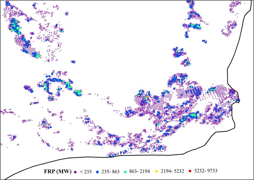
420                                                                       L. Shen et al.: Slump of sea land breeze by aerosols

1   Introduction                                                     from biomass burning (van der Werf et al., 2006; Meyer et
                                                                     al., 2008). Particularly, there have been many studies con-
Aerosols play an important role in balancing the Earth’s ra-         centrating on wild fires’ association with enhancing aerosol
diation budget, through their direct or indirect effects (Al-        loadings and air pollution events in Australia, some of which
brecht, 1989; Garrett and Zhao, 2006; IPCC, 2013; McCoy              included the discussion on the combined effect from back-
and Hartmann, 2015). There are different types of aerosols           ground meteorological conditions (Mitchell et al., 2006;
from various sources which have different climatological             Luhar et al., 2008; Meyer et al., 2008; Mitchell et al., 2013;
forcing effects (Charlson et al., 1992; Yang et al., 2016).          Mallet et al., 2017). The 2019 Australian wild fires from
Aerosols differ in radiative forcing effects as their physical       December 2019 to February 2020 were unprecedented in
and chemical properties vary, some of which may affect the           recent decades in terms of the magnitude and consistency,
earth–atmosphere system by bringing changes to the lifespan          so they have attracted the attention of the world in a short
of clouds (Albrecht, 1989; Zhao and Garrett, 2015).                  time. Since their outbreak, numerous studies have been car-
   Carbonaceous aerosol contains black carbon (BC) and               ried out to investigate them from different aspects. For exam-
organic carbon (OC) and serves as a major radiation-                 ple, Yang et al. (2021) examined the statistical properties of
influencing aerosol which mainly originates from biomass             aerosol properties associated with the 2019 Australian mega
burning (Vermote et al., 2009; Yang et al., 2021). There             fire events in both horizontal and vertical directions. Torres
have been studies addressing the importance of BC on at-             et al. (2020) investigated the aerosol emissions during the
mospheric warming and that of OC on weakening in situ                mega fires happening in New South Wales, Australia, and
downwelling solar radiation (Jacobson, 2001; Ramana et al.,          found a great amount of carbonaceous aerosols in the strato-
2010). There are also some studies that try to quantify the          sphere. Ohneiser et al. (2020) traced wildfire smoke in one of
average radiative forcing effects of BC and OC, while they           the most severely burnt areas in southeastern Australia and
also emphasize the potential uncertainties with respect to the       found that smoke could even travel across the Pacific, which
specific values (Zhang et al., 2017). At a planetary scale, the      was detected by an observation site at Punta Arenas in South
change of aerosols brings many uncertainties to the radia-           America.
tion balance, thus further influencing the magnitude of atmo-           Sea land breeze (SLB) is a common circulation over
spheric circulation (Wang et al., 2015; Zhao et al., 2020). At       coastal areas whose direct cause is the regional temperature
a synoptic scale, aerosols can affect tropical cyclones by en-       difference between land and sea (TDLS). Many studies have
larging their rainfall area, which is also related to their radia-   investigated this regional circulation. On the one hand, the
tive properties (Zhao et al., 2018). At a regional scale, Han        complicated influencing factors of SLB have been studied
et al. (2020) discussed in detail the radiative forcing effect       from different perspectives (Miller et al., 2013). Our previ-
of aerosols on the speed of the urban heat island (UHI) in           ous studies pointed out that the change of TDLS is highly
different seasons.                                                   related to the change of in situ downwelling solar radiation
   As mentioned above, biomass burning is an important               (Shen et al., 2021a, b; Shen and Zhao, 2020). We also found
source of aerosols, especially for carbonaceous aerosols. Ad-        that the continuous increase of surface roughness in cities
equate amounts of fire-emitted aerosols would bring per-             can reduce the SLB speed in the long term (Shen et al., 2019).
turbations to the balanced Earth’s climate system through            The long-term significance and trends of SLBs over the globe
both direct and indirect effects (Jacobson, 2014). There has         are driven by climate regimes which are related to climato-
been much research discussing the characteristics of wild fire       logical differences in both in situ downwelling solar radia-
aerosols and their effect around the world (Grandey et al.,          tion and background wind fields. There are also many other
2016; Mitchell et al., 2006). For example, Portin et al. (2012)      studies on the influencing factors of SLB in short periods.
investigated the characterization of burning aerosols in east-       For example, based on the case analysis, Sarker et al. (1998)
ern Finland during Russian wild fires in the summer of 2010.         found that the UHI magnitude has a great impact on the en-
Kloss et al. (2019) pointed out that wild fires could bring          croachment range of sea wind (SW) frontal surface. Using
plumes of smoke that ascend very high and pollute remote ar-         regional model simulation, Ma et al. (2013) found that the
eas with the help of a monsoon. Grandey et al. (2016) quanti-        UHI effect can greatly enhance TDLS, which would result
fied the radiative effect of the total fire-induced aerosols over    in strengthened SLB circulation in a great metropolis. Miller
the globe, which was estimated to be −1.0 W/m2 on aver-              et al. (2013) reviewed the studies on SLB and pointed out
age. The fire-induced aerosols could have more significant           that local topography such as the shape of the coastline is an-
radiative effects with clouds than under clear-sky conditions        other important influencing factor of SLB. On the other hand,
through cloud–aerosol interaction, whose global forcing ef-          SLB’s effect has also been extensively investigated. For ex-
fect could reach −1.16 W/m2 (Chuang et al., 2002).                   ample, SLB has been reported as a direct controller of air
   Australia is one of the areas where wild fires occur fre-         pollutants which transports air pollutants inland or to the vast
quently (Yang et al., 2021). An area of nearly 550 000 km2           ocean with the help of the background meteorological field
of tropical and arid savanna is burnt each year in Australia,        (Nai et al., 2018; Shen and Zhao, 2020). SLB is also essen-
contributing to about 6 %–8 % of global carbon emissions             tial to the modification of the meteorological conditions and

Atmos. Chem. Phys., 22, 419–439, 2022                                                   https://doi.org/10.5194/acp-22-419-2022
L. Shen et al.: Slump of sea land breeze by aerosols                                                                              421

local climate (Rajib and Heekwa, 2010). Moreover, SLB is            ports, which could possibly have caused fire-induced com-
a determinant factor of the diurnal variation of the precipita-     plex flows and circulation in the form of fire–atmosphere in-
tion on the island since its direction and magnitude can affect     teractions in the vicinity of a fire (Sun et al., 2019). Based
the location and magnitude of convective systems (Zhu et al.,       on previous observation during mega fire events, the concen-
2017).                                                              trated fire spots changed the local air pressure field and added
   Over the years, the cause and effect of aerosols, wild fires     a regional temperature-pressure field, bringing uncertainties
in typical areas and SLBs have been learned in detail. The          to local wind speed and wind direction (Jia et al., 1987; Li et
relationship between aerosols and other small-scale circula-        al., 2016). On the one hand, this could further interrupt the
tions such as UHI circulation has also been investigated from       formation of SLB since it might make the background wind
many aspects (Han et al., 2020). However, few studies have          field more complicated. On the other hand, the detected SLB
investigated the effects of different types of aerosols on SLBs     might not be accurate since it is likely to contain other wind
or looked into how local and remote aerosol emissions dur-          disturbances at a small regional scale.
ing mega fires would affect local SLB with the help of the             As shown in Fig. 1, we selected an urban site in Brisbane
meteorological background field or other potential mecha-           along the eastern coast of Australia as the study site, which
nisms. There was an updated and important study calling for         was due to several considerations. First, alongside the eastern
attention of the record-breaking aerosol emissions during the       coastal areas of Australia which belong to monsoon climate,
2019 Australian mega fires which led to a significant cooling       including Brisbane and areas to its south but to the north of
effect on ocean temperature (Hirsch and Koren, 2021). Since         the fire centre, the Australian monsoon system is not strong,
in situ downwelling solar radiation and sea surface temper-         so the OE-SLB can be verified from a climatological per-
ature (SST), which are both important influential factors of        spective, which also means integrated SLB circulation can
SLB, are deeply affected by different types of aerosols due         be found during all seasons. Second, compared to rural sites,
to their different radiative properties, it is interesting to ex-   there are longer periods of high-time-resolution observation
amine in detail how the record-breaking mega fires would            data at urban sites, which is necessary for the extraction of
influence SLB by releasing large amounts of aerosols.               SLB signals. Third, the urban area of Brisbane is relatively
   The paper is organized as follows. Section 2 describes the       small and is not very far from vast areas of forests which pro-
observation site, data and analysis methods. Section 3 illus-       vide stable combustion environment, ensuring the persistent
trates the characteristics of SLB, the variation of SLB days,       effect of wild fires. Fourth, the UHI effect, which could pos-
the distribution and fire radiative power (FRP) of wild fire        sibly interrupt SLB and bring errors when calculating SLB
spots, the anomaly of observed SW speed, land wind (LW)             magnitude, should be small for the study region consider-
speed and air temperature, the effects of different aerosols        ing the small scale of urban areas. Also, the wild fires near
on SLB’s variation, the analysis on background wind field           suburban areas could further eliminate the UHI effect, even
and the comparison between local fire spots’ and the remote         if it could exist through their heating impact on these areas.
fire centre’s contributions. Section 4 summarizes and dis-          In contrast, the forest site is surrounded by or within great
cusses the findings of the study and proposes a mechanism           amounts of flora where the majority of solar radiation is ab-
of aerosol–SLB interaction during the peak of the 2019 Aus-         sorbed and scattered by leaves, prohibiting the surface heat-
tralian mega fires.                                                 ing by solar radiation and then the formation and detection
                                                                    of SLB. Actually, due to the existence of photosynthesis, the
                                                                    endothermic process of leaves from solar radiation and the
2     Data and methods
                                                                    temperature rise of the “leaf surface” are different from those
2.1    Site
                                                                    of Earth’s surface. As a result, the traditional mechanism of
                                                                    SLB formation is not necessarily applicable when the site is
The 2019 Australian mega fires occurred mainly in the east-         in the forest or quite close to clusters of flora. Coastal sites to
ern and southeastern coastal areas of Australian continent          the north of Brisbane are too far from the fire centre, and they
(Yang et al., 2021). The southeastern parts, including the          are mostly rural sites covered with flora as well. Considering
state of Victoria and the southeastern part of the state of New     all of this, we chose the site of Brisbane Archerfield located
South Wales, belong to a marine climate, where obvious ex-          on the eastern coast of the state of Queensland (Fig. 1) as the
istence of SLB (OE-SLB) is not clearly verified because of          study site.
the influence of strong westerlies and water vapour accompa-
nied with westerlies from the ocean (Shen et al., 2021). Note       2.2   Data
that OE-SLB means that SLB is significant from a climato-
logical perspective. In other words, the SLB can be found           Several types of data have been used in this study, including
during most time of the year. Details of the definition of          land-cover-type data, Modern-Era Retrospective analysis for
OE-SLB can be found in Shen et al. (2021) and are not re-           Research and Applications version 2 (MERRA-2) data, Mod-
peated here. Meanwhile, the wild fire events there were the         erate Resolution Imaging Spectroradiometer (MODIS) data,
most severe with a great density according to numerous re-          ground site observation data, the Fifth Version of European

https://doi.org/10.5194/acp-22-419-2022                                                Atmos. Chem. Phys., 22, 419–439, 2022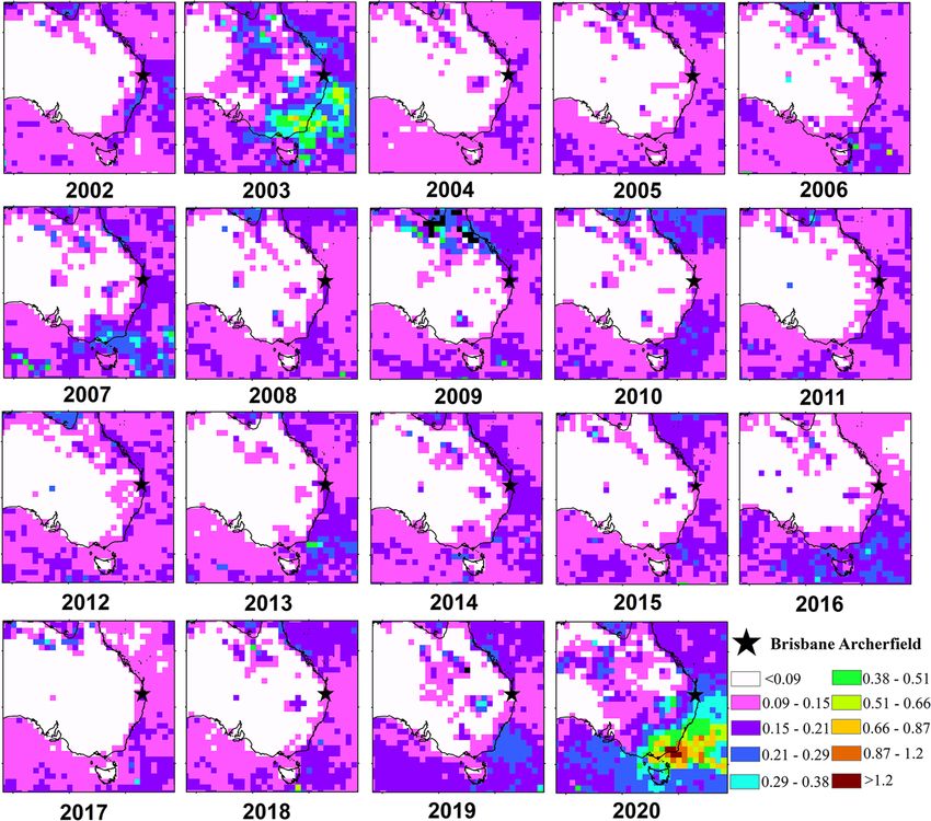
422                                                                      L. Shen et al.: Slump of sea land breeze by aerosols

                                                                    mega fires. The spatial resolution of MERRA-2 AOD data
                                                                    is 0.625◦ × 1◦ .
                                                                       MODIS data. The MODIS instrument is performed
                                                                    on Aqua and Terra platforms. In this study, we used
                                                                    the MODIS cloud product which belongs to the dataset
                                                                    of MCD06COSP_M3_MODIS. The cloud information in-
                                                                    cludes cloud optical depth (COD) and cloud fraction for all
                                                                    January months during the period from 2003 to 2020 with
                                                                    a monthly time resolution. The Brisbane Archerfield site is
                                                                    located at 153.008◦ E, 27.57◦ S. So we used COD and cloud
                                                                    fraction data whose space range and resolution are 152.5–
                                                                    153.5◦ E × 28.5–26.5◦ S and 1◦ × 1◦ respectively. This spa-
                                                                    tial range covers the whole Brisbane area and the normal en-
                                                                    croaching distance of SLB, which is about tens of kilometres
                                                                    (Rajib and Heekwa, 2010; Shen et al., 2019). In this study,
                                                                    their spatial averages were calculated to represent the local
                                                                    COD and cloud fraction every January from 2003 to 2020.
                                                                    Also, we used the MODIS monthly AOD product for com-
                                                                    parison with that of MERRA-2, which belongs to the dataset
                                                                    of MOD08_M3. The spatial resolution of MODIS AOD data
Figure 1. The map of eastern Australia with land-cover types. The   is 1◦ × 1◦ , and the time range is the same as that of MERRA-
observation site is marked by a black dot.                          2.
                                                                       Ground site observation data. The wind and air tempera-
                                                                    ture observation data are from National Oceanic and Atmo-
                                                                    spheric Administration (NOAA) global observation network
                                                                    at the site of Brisbane Archerfield (153.008◦ E, 27.57◦ S). We
Centre for Medium-Range Weather Forecasts (ECMWF) Re-               used data in January from 2001 to 2020 in this study. The
Analysis (ERA5) data, fire spot and FRP data and Global             time resolution is every 3 h at 02:00, 05:00, 08:00, 11:00,
Data Assimilation System (GDAS) data. The detailed data             14:00, 17:00, 20:00 and 23:00 UTC on most days. The con-
information is described below one by one.                          tinuity of the observation data is ensured; there are observa-
   Land-cover-type data. The land-cover-type data of Aus-           tions on each day in January throughout the whole study pe-
tralia are from the Dynamic Land Cover Dataset (DLCD)               riod, with only one missing observation data on each day of
with Version 2.1 provided by Geoscience Australia. In this          a small fraction time (approximately 3.5 %). The wind infor-
study, the DLCD land-cover-type data were used to reveal            mation includes wind speed and wind direction. The air tem-
the surrounding landscape of Brisbane Archerfield. The spa-         perature is measured in Fahrenheit, and we have converted it
tial resolution of the data is 0.002◦ × 0.002◦ , which is based     into Celsius. The observation data were the main data used
on the annual mean of satellite observations from 2014 to           in this study to show the variations of both SLB and air tem-
2015.                                                               perature during the fire.
   MERRA-2 data. MERRA-2 belongs to the global atmo-                   ERA5 data. The monthly mean U wind (zonal) speed and
spheric reanalysis product managed by the National Aero-            V wind (meridional) speed in January 2020 from the ERA5
nautics and Space Administration (NASA). It is produced by          were used in this study to reveal the background meteoro-
the Global Modeling and Assimilation Office (GMAO), and             logical field so as to assess its effect on aerosol transport.
the assimilation system of Goddard Earth Observing Sys-             The spatial resolution is 0.250◦ × 0.250◦ at pressure levels
tem (GEOS-5) is used to ensure the quality of this dataset.         of 1000, 975, 950, 925, 900, 875, 850, 825, 800, 775, 750
At major ground sites over Australia, Yang et al. (2021)            and 700 hPa.
compared the monthly aerosol optical depth (AOD) prod-                 Fire spot and FRP data. Fire spot and FRP data are from
uct with Aerosol Robotic Network (AERONET) observa-                 the MODIS product (MCD14). This product can catch and
tions and found their root mean square errors (RMSEs) were          locate the active fire hotspots based on thermal anomalies of
all smaller than 0.05. Thus, MERRA-2 should be reliable to          1 km pixel resolution (Giglio et al., 2016). The time resolu-
be used for the analysis of the large-scale spatial distribu-       tion is daily, and we used the monthly averages for January
tion of AOD in Australia. Yang et al. (2021) also denoted           from 2002 to 2020 to look into the fire situations over the
that the 2019 Australian mega fires were the strongest in Jan-      years in detail.
uary 2020. Correspondingly, we used the monthly AOD in                 GDAS data. The GDAS data were used to perform the
January at 550 nm from 2002 to 2020 to check the AOD                back-trajectory analysis from the Hybrid Single-Particle La-
difference between the mega fire year and years with no             grangian Integrated Trajectory (HYSPLIT). The spatial res-

Atmos. Chem. Phys., 22, 419–439, 2022                                                 https://doi.org/10.5194/acp-22-419-2022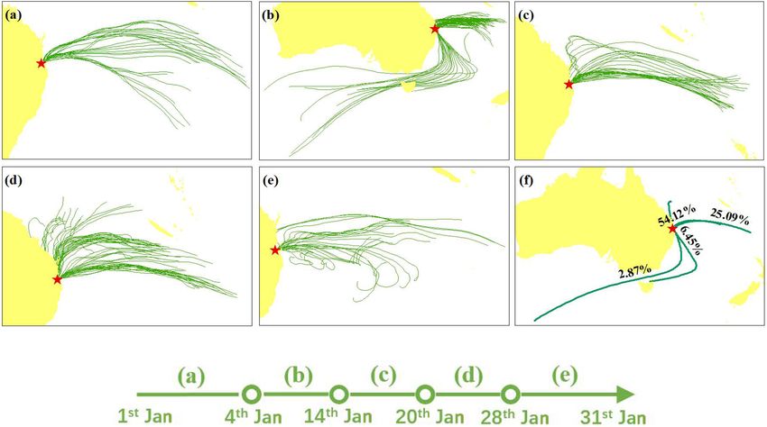
L. Shen et al.: Slump of sea land breeze by aerosols                                                                              423

olution of GDAS data is 1◦ × 1◦ with daily time resolution.
The levels of GDAS data chosen in this study to help to per-
form HYSPLIT analysis were 500 m and 3 km respectively.
The time range set in this study was the whole of January
2020.

2.3     Methods

2.3.1    Extracting SLB signal

The verification of OE-SLB and extraction of SLB signals
from original wind observation over monsoon areas were car-
ried out through the method of the separation of the regional
wind field (SRWF). The definition of OE-SLB, the details of
SRWF method and the criterion for verification were detailed      Figure 2. Hourly average of wind angle in a diurnal period
in our previous studies and are not repeated here (Shen et al.,   (HAWADP) of the local wind.
2019; Shen and Zhao, 2020; Shen et al., 2021). Briefly speak-
ing, SRWF calculates the vector difference between observed       Table 1. Summary of information for the verification of OE-SLB at
wind vector and daily average wind vector for each observa-       Brisbane Archerfield.
tion time. Then, the vector difference is considered to be the
local wind. The criterion of OE-SLB requires that there are        The range of SW   The range of LW      PTS (UTC)       PTL (UTC)
intersection sets among the range of SW, the range of LW and       [20◦ 135◦ ]            [200◦ 315◦ ]   [05:00 08:00]   [14:00 20:00]
the range of hourly average of wind angle in a diurnal period
(HAWADP). Also, the intersection set between the range of
SW (LW) and the range of HAWADP only exists during day-           which means that 05:00–08:00 UTC and 14:00–20:00 UTC
time (night-time). Then the local wind can be thought as the      are within the real PTS and PTL respectively, even if they
SLB signal as long as the OE-SLB is verified at that site.        are not the exact PTS or PTL. Thus, the PTS (PTL) defined
Based on HAWADP and specific sea–land distribution, we            in this study is reliable. The aim of defining PTS (PTL) is
further defined the prevailing time of sea wind (PTS) and         to find the time period when SW (LW) develops most vig-
prevailing time of land wind (PTL). Briefly speaking, during      orously so as to ensure further exclusion of winds from syn-
PTS (PTL) the local wind keeps blowing from sea (land), and       optic scales when trying to extract real SLB signals after ap-
the wind angle keeps rotating towards the direction of vast       plying the SRWF method (Shen and Zhao, 2020; Shen et al.,
sea (inland). The HAWADP at Brisbane Archerfield is shown         2021; Cuxart et al., 2014).
in Fig. 2. As shown, the HAWADP of local wind was close
to sinusoid, which conformed to previous findings in other
                                                                  2.3.2   Definition of the SLB day
monsoon areas (Shen et al., 2021; Yan and Anthes, 1987).
According to the sea–land distribution shown in Fig. 1, we        The SLB day is the day when SLB circulation is most signif-
first defined the ranges of SW and LW, and then the OE-SLB        icant (Xue et al., 1995). To some extent, the number of SLB
of Brisbane Archerfield was verified using these criteria. We     days reveals the activity level of SLB. Different criteria have
further selected the PTS (PTL) based on the rules above.          been adopted when defining the SLB day. Here we referred
    To make it clear, we summarize the range of SW, LW,           to our previous study (Shen et al., 2019) to adopt the criteria
PTS and PTL in Table 1. The ranges of SW and LW re-               based on the minimum times of successful detection of winds
fer to specific sea–land distribution. Notably, there are few     coming from the range of SW (LW) during PTS (PTL). Since
mountains within the ranges of SW and LW based on the             the time interval between two adjacent observations is 3 h,
accurate site location and detailed landscape nearby, which       which makes the number of total observation times less than
helps to exclude potential interruption from other small-         the total hours during prevailing time, we modified the crite-
scale circulations like mountain–valley wind. Note that the       ria slightly as follows: when the offshore land winds occur in
actual PTS (PTL) may be longer than what we defined               the period of 14:00–20:00 UTC with a total occurrence time
here because the time resolution is 3 h instead of hourly in      of no fewer than three times, and the onshore sea winds oc-
this study. As a result, we cannot know the exact thresh-         cur in the period of 05:00–08:00 UTC with a total occurrence
old of time when the wind angle meets the criteria men-           time of no fewer than two times, the day is counted as a SLB
tioned above. For instance, it is possible that the wind an-      day.
gle is within the range of SW before 05:00 UTC. However,
it is still certain that the SW (LW) develops vigorously dur-
ing 05:00–08:00 UTC (14:00–20:00 UTC) based on Fig. 2,

https://doi.org/10.5194/acp-22-419-2022                                              Atmos. Chem. Phys., 22, 419–439, 2022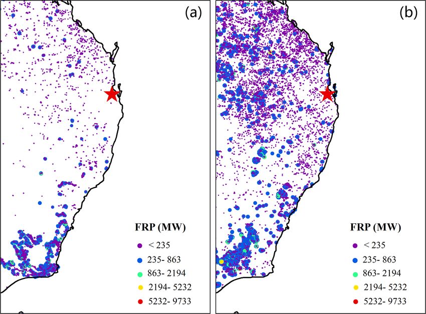
424                                                                       L. Shen et al.: Slump of sea land breeze by aerosols

2.3.3    The calculation of monthly SW and LW speeds
After defining PTS, PTL and SLB day, we could finally cal-
culate the monthly SW and LW speeds. First, we picked up
SLB days in every January from 2001 to 2020. Second, we
picked up local wind speed during PTS (PTL) on SLB days
and calculated the monthly average of SW (LW) speed in ev-
ery January from 2001 to 2020.
   Based on GDAS data throughout the whole of January
2020, the back trajectories of the lower atmosphere at Bris-
bane Archerfield were simulated using the HYSPLIT model,
which could help analyse the effect of background wind
fields on aerosol transport at this site. The simulated levels at
the site were 500 m and 3 km since the lower level of the at-
mosphere (500 m) was closer to fire spots, and there was also
accumulated smoke at 3 km in the southeastern parts of Aus-         Figure 3. Number of SLB days in January from 2001 to 2020.
tralia during the exact same month (Yang et al., 2021). The
TrajStat module of Meteoinfo version 2.4.1 was also used
to cluster the back trajectories based on the Euclidean dis-        2000). Among all the influencing factors, cloud is one of the
tance method, whose details and source code can be found on         most important because it has a significant effect on in situ
its official website (http://meteothink.org/docs/trajstat/index.    solar radiation, which is the direct cause of TDLS. We will
html, last access: 31 January 2021).                                discuss this in the following sections.

2.3.4    The calculation of monthly temperature during
                                                                    3.2   The trends in SW and LW speeds and local air
         daytime and night-time
                                                                          temperature
After defining the SLB day, PTS and PTL, we calculated
the monthly mean temperature during daytime and night-              The monthly mean SW and LW speeds in January from 2001
time using the similar method as SW and LW speeds. First            to 2020 are shown in Fig. 4a. As can be seen, there were
we selected the temperature on SLB days. Second, we cal-            fluctuations in the trends of both SW and LW speeds. The
culated the monthly average of temperature during PTS               SW speed was higher than LW speed, which conformed to
(PTL) to represent monthly average temperature during day-          many previous findings (Miller et al., 2013; Zhu et al., 2017).
time (night-time) in January. Actually, temperature during          The averages were calculated as 3.70 m/s for SW speed and
daytime (night-time) represents land temperature when SW            2.86 m/s for LW speed, respectively. Figure 4b and c show
(LW) prevails. In order to make it clear and concise, we call       the anomalies of both SW and LW speeds. In general, LW
it temperature during PTS (PTL) or land temperature during          speed fluctuated more significantly than SW speed did. This
daytime (night-time) in this study.                                 is due to its lower level of kinetic energy which can make it
                                                                    more sensitive to any potential interruptions from the back-
                                                                    ground meteorological field (Shen and Zhao, 2020). The neg-
3     Results
                                                                    ative anomalies of LW speed happened in 2001, 2004, 2008,
                                                                    2010, 2011, 2015, 2016, 2017, 2018 and 2020. Different
3.1     The variation of SLB day number
                                                                    from other years, it is obvious that the negative anomaly in
Figure 3 shows the SLB day number in January from 2001              2020 was higher than 0.6 m/s, which was beyond the multi-
to 2020. As shown, the SLB day number in January was nor-           years’ oscillation range. The anomaly accounted for 22.3 %
mally larger than 10. Among these 20 years, there were 25 %         of the multi-years’ average LW speed. The negative anoma-
of the years whose SLB days in January accounted for more           lies of SW speed happened in 2004, 2008, 2009, 2010, 2011,
than half of the month. Note that it does not necessarily mean      2013, 2014, 2015, 2017 and 2020 (Fig. 4c). For SW speed,
that there is no SLB on days that are not SLB days. It is ob-       the negative anomaly in 2020 was also obvious, but its value
vious that there was a slump in the number of SLB days in           was still within the multi-year oscillation range. It was higher
2020. The total SLB day number dropped to only 4 during             than 0.5 m/s, accounting for 14.8 % of the multi-years’ aver-
mega fires, accounting for only 33.33 % of the average SLB          age. It is interesting to find that there were obvious positive
day number during the past 20 years. Also, the year 2012            anomalies of both SW and LW speeds in 2003, whereas their
witnessed a low SLB day number (6 d) in January. There are          absolute values were not the highest. Also, the SLB day num-
a lot of potential influencing factors for SLB frequency, such      ber in 2003 was near the average. We will discuss this further,
as the background wind field (Miller et al., 2013) and the          along with the aerosol emissions during that year, in the fol-
interruption of other small-scale circulations (Kusaka et al.,      lowing sections.

Atmos. Chem. Phys., 22, 419–439, 2022                                                  https://doi.org/10.5194/acp-22-419-2022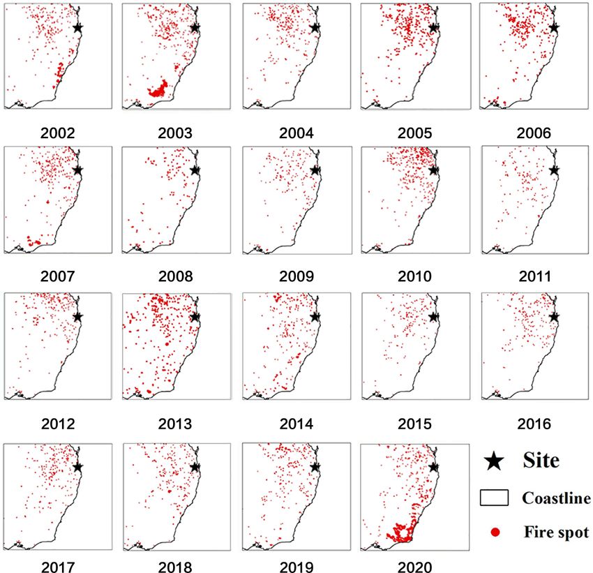
L. Shen et al.: Slump of sea land breeze by aerosols                                                                        425

                                                                    In order to be more accurate, we carried out linear regres-
                                                                 sion between temperature during PTL and LW anomaly and
                                                                 found that they had a negative linear relationship (p < 0.02)
                                                                 with each other (Fig. 5). As the temperature increased by
                                                                 10 ◦ C, the LW speed anomaly decreased by 1.52 m/s. The
                                                                 correlation coefficient R was 0.52, which was at the medium
                                                                 level. However, considering the significance level as well as
                                                                 low level of sample number, it can be concluded that the
                                                                 LW speed is generally negatively correlated with night-time
                                                                 land temperature. Moreover, their R and significance level
                                                                 could be 0.69 and 0.0012 respectively if we excluded the
                                                                 only one abnormal point in 2019, which might be caused by
                                                                 some potential disturbances on coastal SST where the verti-
                                                                 cal stream of SLB lies. Considering all these, it can be con-
                                                                 cluded that the LW speed anomaly is generally negatively
                                                                 correlated with night-time land temperature. During night-
                                                                 time, the land is colder than the sea. As the land temperature
                                                                 increases, the TDLS decreases if the SST of the area where
                                                                 the upward stream of SLB lies remains relatively stable; the
Figure 4. The trends of SW and LW speeds (a), the LW speed
                                                                 LW speed does too. Briefly, the good linear relationship re-
anomaly and land temperature during night-time (b) and the SW
                                                                 veals that the variation of temperature during PTL (night-
speed anomaly and land temperature during daytime (c) based on
their monthly average during January from 2001 to 2020.
                                                                 time land temperature) could generally represent the varia-
                                                                 tion of TDLS during PTL, while the daytime land tempera-
                                                                 ture variation could not represent the TDLS variation during
                                                                 PTS. In our previous study, we also found through obser-
   It can be seen in Fig. 4b that there were also significant    vation that the daily lowest temperature (DLT) was clearly
fluctuations in night-time land temperature over the years.      negatively related to LW speed, while the SW speed was
There was a soar in land temperature during night-time in        more related to in situ downwelling solar radiation rather
2020 which approached nearly 24 ◦ C. It was nearly 3 ◦ C         than merely land temperature (Shen et al., 2021), which was
higher than the multi-years’ average, exceeding the range of     similar to the findings here. It could be inferred that although
multi-years’ oscillation. The fluctuation in land temperature    the land temperature during daytime increased during mega
during daytime was less significant than that during night-      fire events, TDLS was still narrowed during fire events. If
time. There was an obvious positive anomaly in 2020, in-         we only consider the land temperature, the SW speed should
dicating that the daytime land temperature was higher than       have increased during fire events because SW circulation is
that in normal years. Meanwhile, it was still within the range   formed due to warmer land and colder sea. Consequently,
of multi-years’ oscillation, though the positive anomaly was     there should be other factors which could cause decreased
obvious. Fire spots have a heating effect on the nearby en-      TDLS during PTS, which is the direct cause of decreased SW
vironment through either shortwave radiation of light from       speed. We would investigate this in the following sections.
fires or heat conduction caused by a temperature gradient.
It can be inferred that the mega wild fires in January 2020      3.3   The distribution and FRP of fire spots
contributed to the positive temperature anomalies during PTS
(PTL) through the heating effect of fires, though they might     Since the heating effect depends largely on the distance be-
not be the only cause. The heating effect during mega fires      tween the area heated and the heat centre, it is necessary
was more significant during night-time than during daytime,      to examine the distribution of fire spots in January over the
which is probably due to a colder background temperature         years, which is shown in Fig. 6. It can be seen that fire spots
field during night-time.                                         are scattered all over the eastern part of Australia in January
   Basically, the decreased SW (LW) speed revealed that the      over the years. January is the middle of Australian summer,
TDLS during PTS (PTL) decreased. To be more specific, the        which is the season when wild fires happen most frequently
temperature difference between the small regions where the       (Yang et al., 2021). Apart from 2020, other years also wit-
upward stream and downward stream of SLB circulation lie         nessed considerable scattered fire spots all over the coastal
became smaller during January 2020. Based on Fig. 4b and         and inland regions. It is obvious that there was an extreme
c, temperature during PTL seems to be generally negatively       fire centre in the southeastern corner of Australia with a great
related to LW speed anomaly, while it is obvious that tem-       density of fire spots in January 2020. This was exactly the re-
perature during PTS does not show any corresponding rela-        gion where the 2019 Australian mega fires mainly happened.
tionship with SW anomaly.                                        To be specific, it was the eastern corner of the state of Vic-

https://doi.org/10.5194/acp-22-419-2022                                            Atmos. Chem. Phys., 22, 419–439, 2022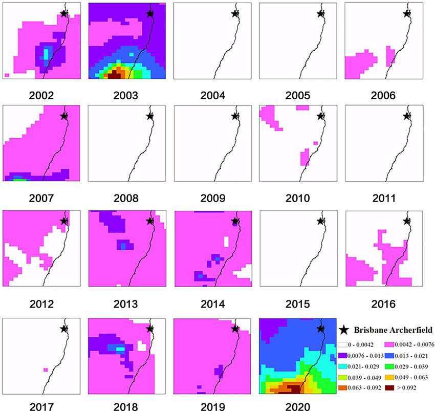
426                                                                           L. Shen et al.: Slump of sea land breeze by aerosols

Figure 5. The relationship between LW anomaly and temperature
during PTL based on their monthly average during January from
2001 to 2020.                                                           Figure 7. The fire radiative power (FRP) of total fire spots in east-
                                                                        ern Australia during January 2020 (a) and January from 2002 to
                                                                        2019 (b).

                                                                           There is another possibility that although the fire spots
                                                                        nearby the site were not more concentrated with great den-
                                                                        sity in 2020 than in other years, the FRP of fire spots in 2020
                                                                        was higher. This means that the fire was greater regardless of
                                                                        the ordinary density of spots, which could also result in more
                                                                        fire-induced aerosol emissions. So we further examined the
                                                                        FRP of fire spots in 2020 and those in other years. In or-
                                                                        der to make it comparable and verifiable, the time period of
                                                                        data chosen here was the same as that in Fig. 6. As shown in
                                                                        Fig. 7a, both the nearby and local fire spots in 2020 were
                                                                        mostly within the lowest FRP range, which was less than
                                                                        235 MW. There were some sparse fire spots with greater FRP
                                                                        (235–863 MW) scattered all over the eastern part of Aus-
                                                                        tralia. The FRP of the fire centre was higher than the FRP
                                                                        of other fire spots; there were many fire spots with greater
                                                                        FRP which belonged to the range of 235–863 MW or 863–
                                                                        2194 MW. Figure 7b shows the FRP of all fire spots from
                                                                        2002–2019. The FRP of nearby or local fire spots also had
Figure 6. The fire spot distribution in eastern Australia during Jan-   the lowest values. As the number of years increased, the den-
uary from 2002 to 2020.                                                 sity of fire spots with higher FRP (235–863 MW) increased
                                                                        significantly, most of which were located in inland areas of
                                                                        the Australian continent. This indicates that scattered wild
                                                                        fires with low or medium FRP are common in Australia, but
toria and the southeastern corner of the state of New South             concentrated mega fires are not so common. There were also
Wales, which is in agreement with many reports in the me-               some fire spots which belonged to the range of 235–863 MW
dia. There was also a great fire centre in the southeastern             or 863–2194 MW in 2003, yet the number was less, and the
corner in 2003, although the scale was smaller than that in             distribution areas were smaller. Based on Fig. 7, one impor-
2020. Considering the distribution of fire spots near the site,         tant point we found is that there was no discrepancy between
the density of fire spots nearby was not higher than in other           FRP of nearby or local fire spots in 2020 and that of nearby
years. Instead, there seems to be more fire spots nearby the            or local fire spots in other years. So the possibility mentioned
site in 2003, 2005, 2006, 2010 and 2013 in the figure. If we            above was discarded.
restrained the nearby region to areas of smaller scales, the               Based on the analysis above, the nearby fire spot density
year 2003 and 2013 rather than 2020 would have the most                 and FRP in 2020 were both at the same level as in other years
nearby fire spots.                                                      for local regions near the site. This implies that the heating

Atmos. Chem. Phys., 22, 419–439, 2022                                                       https://doi.org/10.5194/acp-22-419-2022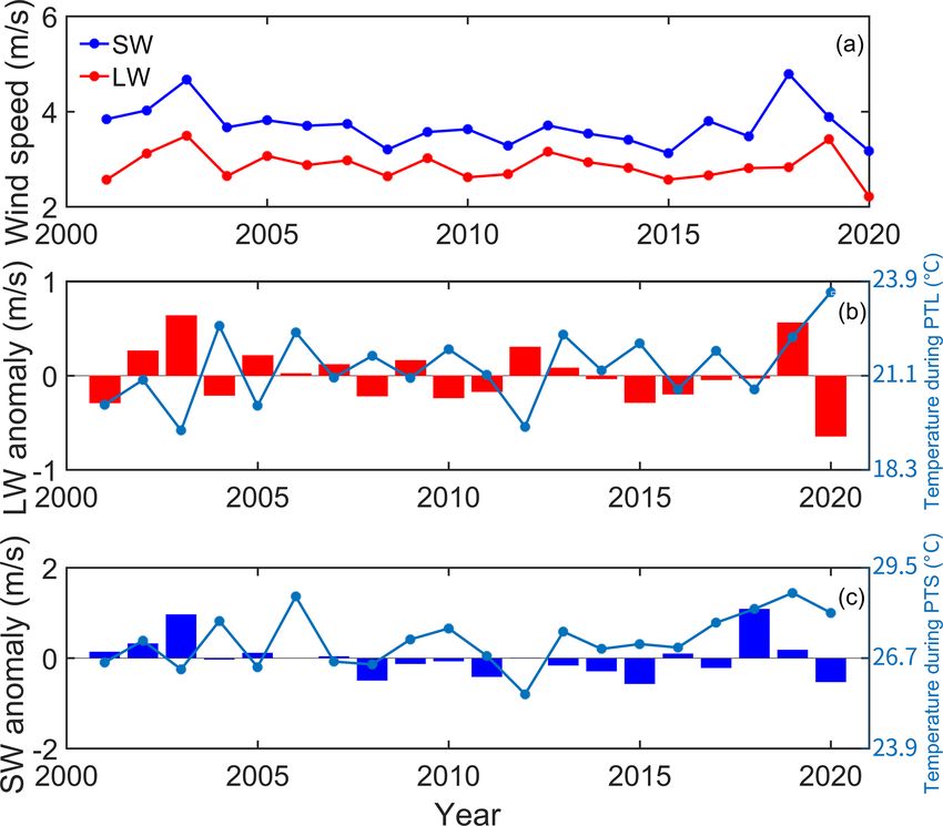
L. Shen et al.: Slump of sea land breeze by aerosols                                                                          427

effect of nearby fire spots did exist in 2020, contributing to      during mega fires, and it has higher spatial resolution than
the increase of land temperature to some extent (especially         MODIS. Considering all these aspects and the focus of the
night-time land temperature), but it was not likely the major       study, we used the MERRA-2 product in the analysis on
cause of the land temperature anomaly. Fluctuation in land          local aerosol variations in the following sections. Figure 8
temperature might be caused by combined mechanisms, in-             shows that the background level of TA-AOD was generally
cluding some other potential factors. In other words, the heat-     low in Australia over the years, implying that Australia was
ing effect of fire spots does not necessarily correspond to the     less polluted as a result of human activities. The TA-AOD
observed air temperature increase. For example, Fig. 4b and         in 2020 increased significantly compared with the average
c show that there were negative land temperature anomalies          level. It can be seen that there was a maximum value centre
in 2003, but actually this year witnessed a greater density of      in the southeast corner, which overlapped the region of the
nearby or local fire spots. In a real situation, the scale of SLB   fire spots’ centre (Fig. 6). The peripheral area of the maxi-
is quite small. The fire spots might be quite a long distance       mum value centre was covered with isopleths, showing the
away from the area where the vertical stream of SLB lies, as        characteristics of free diffusion of aerosols in the air. There
a result of which the heating effect is weak.                       was also a maximum value centre in 2003 whose scale was
                                                                    smaller, overlapping the smaller region of the fire centre in
3.4   The spatial distribution of aerosols
                                                                    2003. Based on findings from these three aspects, it can be
                                                                    concluded that the mega fire centre was the main source of
Large fires have great aerosol emissions which affect the           the large amounts of aerosols around the site location. In gen-
in situ solar radiation and then the radiation budget. Based        eral, the TA-AOD was about 240 % of the multi-years’ aver-
on the basic physical mechanism of SLB formation, the ob-           age level at the site, while the TA-AOD in the fire centre was
served decreased SW and LW speeds demonstrated the de-              at a more astonishing level, accounting for more than 420 %
creased TDLS. As mentioned above, the heating effect of             of that at the local site of Brisbane. Aerosol could signifi-
nearby fire spots was weak and did not become more signif-          cantly affect the in situ downwelling solar radiation through
icant in 2020. So the more important factors bringing about         direct radiative forcing. Turnock et al. (2015) calculated the
the decrease of SW and LW speeds should be more closely             relationship between AOD and surface solar radiation (SSR)
related to TDLS rather than the land temperature only. The          and found that when the background value is low over the
TDLS during SLB formation is highly related to the in situ          years, the SSR increases by 10 % as AOD varies from 0.32 to
downwelling solar radiation. As the shortwave radiation in-         0.16. In this study, the TA-AOD increased even more signif-
creases, the TDLS becomes larger due to the different heat          icantly (240 %), considering the low background value. Nor-
capacities between land and sea. SW forms and prevails              mally, when we talk about the radiative forcing of aerosols in
when TDLS is enough to drive this thermodynamic circula-            the form of SSR difference, it means the instantaneous radia-
tion. During night-time, the land–sea system is a “heater” for      tive forcing. However, the formation of SLB is the result of
the upper atmosphere as the land and sea both give out heat         different levels of radiation accumulations between the land
and undergo energy loss in the form of longwave radiation.          and sea. So the effect of aerosols on the total in situ down-
As the outgoing longwave radiation increases, the TDLS also         welling solar radiation can further accumulate in the process
becomes larger due to the different heat capacities between         of SLB formation and results in even more significant im-
the land and sea. Then the LW forms in a similar way to SW.         pacts on the change of surface temperature.
   Based on discussions above, in situ downwelling solar ra-           Apart from aerosols, clouds could play an even more im-
diation is a crucial influencing factor of SW speed. Consider-      portant role in the radiation budget. The COD and cloud frac-
ing that aerosol is an important factor affecting in situ down-     tion anomaly at this site are shown in Fig. 10. The time range
welling solar radiation, it is necessary for us to check the        was from 2003 to 2020 due to data availability. It can be seen
temporal and spatial variations of aerosols over the years.         that both the cloud fraction and COD in 2003 were at an obvi-
Figures 8 and 9 show the spatial distribution of AOD of             ous low level, while both the cloud fraction and COD in 2020
total aerosols (TA-AOD) over the years using MERRA-2                showed a tiny negative anomaly. Based on the spatial distri-
and MODIS aerosol products, respectively. It shows that             bution of TA-AOD, both 2003 and 2020 witnessed a soar in
except for a little overestimation of AOD in the fire cen-          TA-AOD at the site, while TA-AOD increased more signif-
tre in 2020, the overall distribution and value of AOD re-          icantly in 2020. Figure 3 shows that there was a slump in
vealed by MERRA-2 agreed well with those revealed by                SLB number in 2020 but not in 2003, while Fig. 4 shows that
MODIS. Both MERRA-2 and MODIS show that there was                   there were positive anomalies of both SW and LW speeds
a burst of aerosols in the fire centre during January 2003          in 2003. Many previous studies on SLB have pointed out
and 2020, and the latter was much more severe. Especially           that a high level of in situ downwelling solar radiation is
for the site learned in this study, the difference of AODs          favourable for SLB formation and SLB speed increase (Shen
between MERRA-2 (approximately 0.26) and MODIS (ap-                 and Zhao, 2020; Shen et al., 2021b; Miller et al., 2013).
proximately 0.29) was very small. Thus, MERRA-2 agreed              Our previous study in a monsoon climate region also showed
well with both MODIS and AERONET in terms of AOD                    that there was a positive linear relationship between in situ

https://doi.org/10.5194/acp-22-419-2022                                               Atmos. Chem. Phys., 22, 419–439, 2022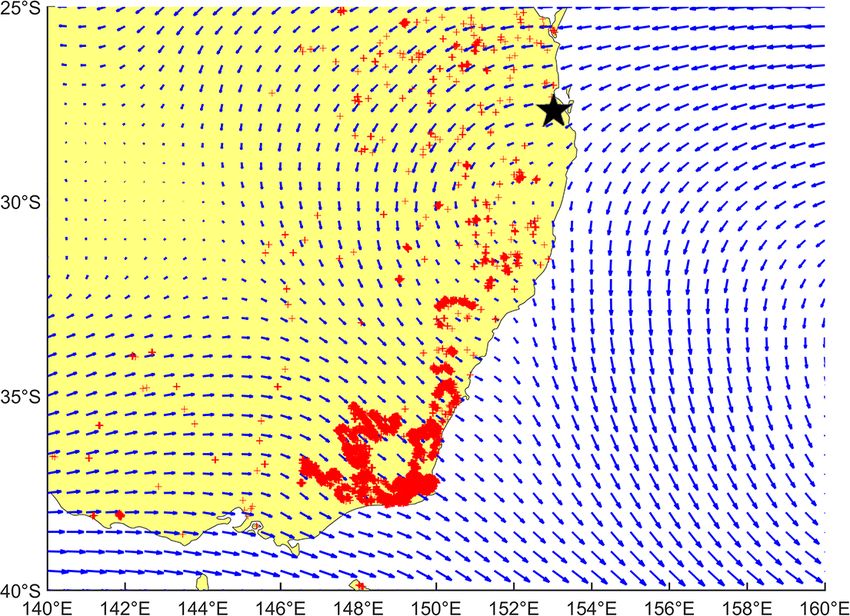
428                                                                          L. Shen et al.: Slump of sea land breeze by aerosols

Figure 8. The spatial distribution of aerosol optical depth (AOD) of total aerosols in eastern Australia during January from 2002 to 2020
using the Modern-Era Retrospective analysis for Research and Applications version 2 (MERRA-2) AOD product.

downwelling solar radiation and SW speed (Shen and Zhao,               and BC. The OC is a very good scatter to solar radiation.
2020). As we know, the in situ downwelling solar radiation             Thus, among all the aerosols, OC could be an important con-
is determined by both cloud and aerosols through their com-            tributor to the weakened TDLS during SW formation. Fig-
bined “umbrella effect”. The finding shown in Figs. 3 and 4            ure 11 shows the spatial distribution of OC over the years.
could be explained by the radiative cooling effects of aerosols        The spatial distribution of OC was also similar to the fire spot
and clouds. Although there was a positive anomaly of TA-               distribution, which further confirmed that the source of great
AOD in 2003, the COD and cloud fraction were less than                 aerosol emissions was the mega fire centre. There were ex-
the average, offsetting the aerosols’ negative radiative forc-         treme value centres in the fire centre in both 2003 and 2020.
ing effect. In situ downwelling solar radiation of the regional        The same as what we found earlier, it can be seen that the
sea–land system was still ensured so that the SLB happened             large values spread further in 2020 than 2003, indicating that
with a normal frequency (Fig. 3) and with an even larger               the fire events were more severe in 2020 than in 2003. Simi-
speed (Fig. 4). The in situ downwelling solar radiation in Jan-        larly, the background value of OC at the site was low on aver-
uary 2020 should be lower than the average, considering the            age. The specific value of organic carbon AOD (OC-AOD) at
tiny negative anomaly in both COD and cloud fraction and               the Brisbane site in 2020 was about 630 % of the multi-years’
the significant increase in TA-AOD. The increased radiative            average, which was even higher than that of total aerosol.
forcing effect of TA-AOD was accumulated during the for-               This is easy to understand because the fire centre is also
mation of SW. In conclusion, during daytime, the negative              covered with plants and trees, and their combustion can re-
radiative forcing effect of total aerosols was the determinant         sult in significant amounts of carbonaceous aerosols. Zhang
factor to weaken the in situ downwelling solar radiation, re-          et al. (2017) estimated the radiative forcing of OC glob-
sulting in lower level of TDLS and then decreased SW speed.            ally using the BCC_AGCM2.0_CUACE/Aero model, which
   Mega fire events are significant in the way that they emit          showed that Brisbane was within the large value area, with
large amounts of carbonaceous aerosols, which include OC               high levels of negative radiative forcing at the top of at-

Atmos. Chem. Phys., 22, 419–439, 2022                                                     https://doi.org/10.5194/acp-22-419-2022
L. Shen et al.: Slump of sea land breeze by aerosols                                                                                429

Figure 9. The spatial distribution of aerosol optical depth (AOD) of total aerosols in eastern Australia during January from 2002 to 2020
using the Moderate Resolution Imaging Spectroradiometer (MODIS) AOD product.

                                                                       mosphere. They also attributed this to biomass combustion.
                                                                       Thus, both total aerosol and OC made great contributions to
                                                                       the SW speed decrease by decreasing in situ downwelling
                                                                       solar radiation in January 2020.
                                                                          The result above is analysed based on the impacts of
                                                                       aerosols on solar radiation. However there is almost no short-
                                                                       wave radiation during night-time. Then one question pops
                                                                       up: why was the slump of LW speed more significant? This
                                                                       indicated that the TDLS was significantly weakened at night
                                                                       in January 2020. While the heating effect of fire spots on
                                                                       night-time land temperature did exist, which was more sig-
                                                                       nificant than that during daytime, it was not likely the main
                                                                       cause of weakened TDLS based on FRP and fire spot distri-
                                                                       bution analysis. We next investigated the spatial distribution
                                                                       of BC over the years in Fig. 12. It shows that the black carbon
                                                                       AOD (BC-AOD) at the site was about 425 % of the multi-
                                                                       years’ average level, with the extreme value centre overlap-
                                                                       ping the area of that of fire spots’ density. Similar to the dis-
                                                                       tribution of TA-AOD and OC-AOD, the peripheral areas of
                                                                       the maximum value centre are covered with isopleths, show-
Figure 10. The monthly cloud optical depth (COD) anomaly and           ing the characteristics of free diffusion. BC is well known
cloud fraction anomaly at Brisbane Archerfield during January from
                                                                       as a kind of absorbing aerosol, which is reported to have a
2003 to 2020.
                                                                       wider range of absorbing band than greenhouse gases, which
                                                                       can absorb broadband radiation from visible light to infrared
                                                                       wavelength (Zhang et al., 2017). During the daytime, it can

https://doi.org/10.5194/acp-22-419-2022                                                   Atmos. Chem. Phys., 22, 419–439, 2022
430 L. Shen et al.: Slump of sea land breeze by aerosols Figure 11. The spatial distribution of aerosol optical depth (AOD) of organic carbon (OC) in eastern Australia during January from 2002 to 2020. absorb solar radiation, longwave radiation from the warmer Another potential contributing accelerator is CO2 , which land and shortwave radiation from local fires. During night- is also the product of fires due to the combustion of plants time, it has a warming effect on both the atmosphere and and trees. CO2 is a kind of greenhouse gas which is likely to Earth’s surface through longwave radiation. As a result, it be engaged in the same mechanism as BC to reduce TDLS has a warming effect on the Earth–atmosphere system, in- during night-time, except that CO2 cannot affect the down- cluding the surface of the regional land–sea system, so there welling solar radiation. Details about this are not repeated is a soaring of temperature, shown in Fig. 4b. The soaring again. However we should note that the effect of CO2 is BC during the mega fire heated the local atmosphere, which based on theoretical analysis rather than observational verifi- was like adding a heater in the air. The heater then gave out cation due to the lack of accurate observation data. Both BC downward longwave radiation to the regional land–sea sys- and CO2 ’s warming effects increase TDLS during daytime, tem. Just like the Sun during daytime, this could trigger a SW which partially offsets the strong negative radiative forcing circulation anomaly, weakening LW circulation. Considering effect of total aerosols, but their combined warming effect is the BC burst during mega fires, there is nothing weird about more significant during night-time than during daytime. That its dominant role in the local land temperature increase dur- is most likely the reason (at least partially) that SW speed had ing night-time. The mechanism proposed above can be sum- a negative anomaly but was less significant than LW speed. marized as follows. During night-time, the formation of LW What we discussed above are all factors whose influences originates from the process of heat release from both land were restrained to a small scale. Although SLB is a small- and sea. As they both lose heat at different paces due to dif- scale system, it can still be affected by the variations of ferent heat capacities, the TDLS is enlarged. During the mega signals on a large scale, since the local temperature is af- fires, the upper atmosphere of the regional land–sea system is fected by both regional forcing and the variation of the large- heated, so that the vertical temperature gradient is weakened, scale background temperature field. In our previous study, which is unfavourable for heat release from both sea and land we weighed their contributions qualitatively (Shen et al., surfaces. As a result, the TDLS is significantly weakened. 2019). In this study, we simply discuss the potential effect Atmos. Chem. Phys., 22, 419–439, 2022 https://doi.org/10.5194/acp-22-419-2022
L. Shen et al.: Slump of sea land breeze by aerosols                                                                               431

Figure 12. The spatial distribution of aerosol optical depth (AOD) of black carbon (BC) in eastern Australia during January from 2002 to
2020.

of the change in large-scale SST. Hirsch and Koren (2021)             The negative radiative forcing effect of total aerosols was the
emphasized the effect of record-breaking aerosol emission             determinant cause for TDLS decrease during daytime, which
from this mega fire on the cooling of the oceanic areas. On           could only be partially offset by other factors.
a large scale, its average radiative forcing on sea surface was
−1.0 ± 0.6 W/m2 . The temperature decrease of large-scale
sea surface could have negative forcing on the SST at a re-           3.5     Source of aerosols
gional scale, though the specific temperature variation of the
sea surface where the SLB vertical stream lies might not be           3.5.1    Fire centre’s emission
the same.
                                                                      As indicated earlier, the year 2020 did not have advantages
   We summarized all the influencing factors of TDLS at both
                                                                      over other years in terms of local and nearby fire spot den-
regional and large scales in Table 2. Among all these fac-
                                                                      sity and FRP in January. Note that certain land-cover types
tors, aerosols, BC, OC and CO2 had direct forcing on TDLS
                                                                      could also increase the aerosol emissions. For example, if
by changing the solar radiation reaching the regional sea–
                                                                      there was more combustible land cover such as forests or
land system. In contrast, the heating effect of fire spots and
                                                                      plants, the fires could emit more carbonaceous aerosols in
large-scale SST signal had forcing on land temperature and
                                                                      the form of smoke. Considering this possibility, we fur-
regional SST respectively, thus further having different forc-
                                                                      ther checked the latest version of land cover in Australia
ing effects on TDLS during daytime and night-time. During
                                                                      online (http://maps.elie.ucl.ac.be/CCI/viewer/index.php, last
the 2019 Australian mega fires, TDLS during daytime and
                                                                      access: 1 April 2021). It was updated to 2019, which over-
night-time both decreased under their combined forcing ef-
                                                                      lapped with the starting time of the 2019 Australian mega
fects, which could be inferred from the anomalies of SLB
                                                                      fires. It showed that the areas and density of flora near the
speed. Clearly, the directions of all forcing effects of different
                                                                      site were stable over the years, implying that the soaring in
factors were the same during night-time. That was why LW
                                                                      local aerosols during mega fires was not likely caused by the
speed decreased much more significantly than SW speed did.
                                                                      change of land cover either.

https://doi.org/10.5194/acp-22-419-2022                                                  Atmos. Chem. Phys., 22, 419–439, 2022
432 L. Shen et al.: Slump of sea land breeze by aerosols
Table 2. Summary of the effect of different factors on TDLS. Factors marked in bold represent that they are either a weak factor or a potential
factor derived from theoretical analysis but not verified by observation.
Influencing factors Forcing on daytime TDLS Forcing on night=time TDLS
Large-scale forcing Cooling of SST on a large scale (Hirsch + −
and Koren, 2021)
Regional forcing Heating effect of nearby fire spots + −
Total aerosols − ×
BC + −
OC − ×
CO 2 + −
As Figs. 6, 8, 11 and 12 show, the distributions of fire
spots, TA-AOD, BC-AOD and OC-AOD were quite similar
to each other. In the fire centre, both the density and FRP of
fire spots were much higher in January 2020 than in January
of other years, which are all based on distribution character-
istics at a large scale. In order to show the fire situation at the
fire centre more accurately, we magnified the FRP map to re-
strain the areas to merely the fire centre, which is shown in
Fig. 13. As shown, the fire spot density was quite high in this
region, especially along coastal areas. Compared with other
areas, the fire centre had much more fire spots with higher
FRP. The spots with FRP from 235 to 864 MW were evenly
distributed in all fire areas, surrounded by low FRP spots
with high density. There were quite a few spots with even
higher FRP ranging from 864 to 2194 MW, which could not
be found in other peripheral areas (Fig. 7a). In some areas at Figure 13. The detailed distribution of fire spots and their FRP in
the fire centre, we could even find fire spots with FRP rang- the fire centre during January 2020.
ing from 2194 to 5232 MW. All these distribution character-
istics of fire spots suggest the possibility of large amounts of
aerosols including smoke being emitted into the atmosphere,
ing the 2019 Australian mega fires and found most of them
after which a great concentration gradient in the horizontal
accumulated under 3 km, which is about 700 hPa. Figure 14
direction is formed between the fire centre and farther ar-
shows the monthly average background wind field based on
eas. Based on basic chemistry law, irreversible free diffusion
wind information at pressure levels from 1000 to 700 hPa in
would happen in this process. As the concentration gap in-
January 2020. The red cross symbols represent the fire spots
creases, the diffusion efficiency also increases. The distribu-
in this figure. The average background wind field clearly re-
tion of contour lines in Figs. 8, 11 and 12 also shows the
vealed the existence of the Southern Hemisphere’s westerlies
characteristics of free diffusion. A similar mechanism works
and a subtropical high. The fire centre was approximately lo-
out for the spatial distribution of CO2 during the fire events.
cated at the intersection of the northern boundary of the west-
erlies and the southwestern boundary of the subtropical high.
3.5.2 Analysis on the background wind field Since January is the middle month of Australian summer, the
subtropical high developed quite vigorously, some of which
Apart from free diffusion, wind is crucial for pollution trans- stretched into the eastern part of the Australian continent.
port including aerosols (Walcek, 2002). Also, wind is a key It covered the areas where most fire spots were located. At
factor of the near-surface CO2 distribution (Cao et al., 2017). a large scale, this caused quite a hot and dry background
Zhang et al. (2017) confirmed that BC could be transported meteorological field, which was favourable for the develop-
over long distances in mid-latitude areas. The transport dis- ment and persistence of wild fires. Based on the average sta-
tance of OC was even longer than that of BC. It is necessary tus of wind fields at different pressure levels, the subtropi-
for us to look into the background wind field in order to know cal high and westerlies together formed a background wind
the likely aerosol transport from the fire centre to the site. field blowing from the site to the fire centre, which was un-
Yang et al. (2021) retrieved the average status of the vertical favourable for the aerosol transport from the fire centre to
distribution of various aerosols in southeastern Australia dur- the site. However, we should notice that this figure merely
Atmos. Chem. Phys., 22, 419–439, 2022 https://doi.org/10.5194/acp-22-419-2022You can also read