On the circulation, water mass distribution, and nutrient concentrations of the western Chukchi Sea
←
→
Page content transcription
If your browser does not render page correctly, please read the page content below
Ocean Sci., 18, 29–49, 2022
https://doi.org/10.5194/os-18-29-2022
© Author(s) 2022. This work is distributed under
the Creative Commons Attribution 4.0 License.

On the circulation, water mass distribution, and nutrient
concentrations of the western Chukchi Sea
Jaclyn Clement Kinney1 , Karen M. Assmann2,3 , Wieslaw Maslowski1 , Göran Björk2 , Martin Jakobsson4 ,
Sara Jutterström5 , Younjoo J. Lee1 , Robert Osinski6 , Igor Semiletov7 , Adam Ulfsbo2 , Irene Wåhlström8 , and
Leif G. Anderson2
1 Naval  Postgraduate School, 833 Dyer Rd., Monterey, CA 93943, USA
2 Department   of Marine Sciences, University of Gothenburg, 405 30 Gothenburg, Sweden
3 Institute of Marine Research, P.O. Box 6606 Stakkevollen, 9296 Tromsø, Norway
4 Department of Geological Sciences, Stockholm University, 106 91 Stockholm, Sweden
5 IVL Swedish Environmental Research Institute, P.O. Box 530 21, 400 14 Gothenburg, Sweden
6 Institute of Oceanology, Polish Academy of Sciences, 81-712 Sopot, Poland
7 Pacific Oceanological Institute, Russian Academy of Sciences Far Eastern Branch, Vladivostok 690041, Russia
8 Swedish Meteorological and Hydrological Institute, Norrköping, Sweden

Correspondence: Jaclyn Clement Kinney (jlclemen@nps.edu) and Leif G. Anderson (leif.anderson@marine.gu.se)

Received: 11 May 2021 – Discussion started: 25 May 2021
Revised: 12 November 2021 – Accepted: 16 November 2021 – Published: 5 January 2022

Abstract. Substantial amounts of nutrients and carbon en-         by combining hydrographic and nutrient observations with
ter the Arctic Ocean from the Pacific Ocean through the           geostrophic transport referenced to lowered acoustic Doppler
Bering Strait, distributed over three main pathways. Water        current profiler (LADCP) and surface drift data. Even if there
with low salinities and nutrient concentrations takes an east-    are some general similarities between the years, there are dif-
ern route along the Alaskan coast, as Alaskan Coastal Water.      ferences in both the temperature–salinity and nutrient charac-
A central pathway exhibits intermediate salinity and nutrient     teristics. To assess these differences, and also to get a wider
concentrations, while the most nutrient-rich water enters the     temporal and spatial view, numerical modelling results are
Bering Strait on its western side. Towards the Arctic Ocean,      applied. According to model results, high-frequency variabil-
the flow of these water masses is subject to strong topo-         ity dominates the flow in Herald Canyon. This leads us to
graphic steering within the Chukchi Sea with volume trans-        conclude that this region needs to be monitored over a longer
port modulated by the wind field. In this contribution, we use    time frame to deduce the temporal variability and potential
data from several sections crossing Herald Canyon collected       trends.
in 2008 and 2014 together with numerical modelling to in-
vestigate the circulation and transport in the western part of
the Chukchi Sea. We find that a substantial fraction of wa-
ter from the Chukchi Sea enters the East Siberian Sea south       1   Introduction
of Wrangel Island and circulates in an anticyclonic direction
around the island. This water then contributes to the high-       The Arctic Ocean has experienced large changes in recent
nutrient waters of Herald Canyon. The bottom of the canyon        decades with a decrease in summer sea ice cover as the most
has the highest nutrient concentrations, likely as a result of    prominent, impacting a number of processes including the
addition from the degradation of organic matter at the sedi-      functioning of the ecosystem (e.g. Meier et al., 2014; Kwok,
ment surface in the East Siberian Sea. The flux of nutrients      2018). More open water decreases the albedo which ampli-
(nitrate, phosphate, and silicate) and dissolved inorganic car-   fies warming (Kashiwase et al., 2017). To some degree, this
bon in Bering Summer Water and Winter Water is computed           change in albedo is compensated for by more cloud forma-
                                                                  tion caused by increased evaporation from the open water.

Published by Copernicus Publications on behalf of the European Geosciences Union.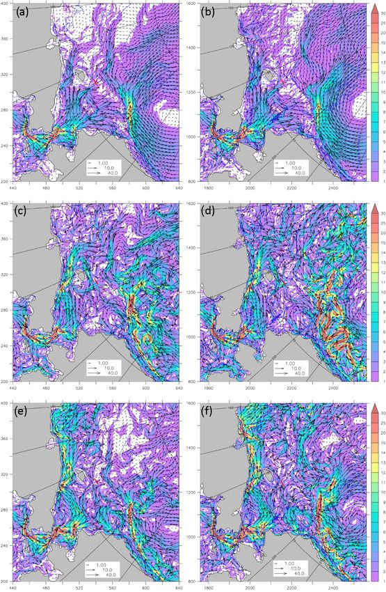
30                  J. Clement Kinney et al.: On the circulation and water mass distribution of the western Chukchi Sea

The melting of sea ice is mainly caused by atmospheric forc-        the Bering Strait to form what is known as Bering Summer
ing (Ding et al., 2017), but inflow of warm surface water           Water (e.g. Pisareva et al., 2015). These water masses largely
from the Atlantic and Pacific oceans (see Fig. 1a for the gen-      take different paths in the Chukchi Sea before entering the
eral circulation) also plays a role, as well as the heat mixed      deep central Arctic Ocean (Brugler et al., 2014) (Fig. 1b),
up into the surface ocean from deeper layers (e.g. Polyakov         but mixing between these and other waters, like the water of
et al., 2013, 2017; Stroeve and Notz, 2018). The tempera-           the Siberian Coastal Current (SCC), occurs (e.g. Weingartner
ture of the Atlantic Water entering the Arctic Ocean through        et al., 1999). In general, Alaskan Coastal Water follows the
the Fram Strait has varied over the last decade with an in-         coast towards Barrow Canyon, while Bering Summer Water
creasing trend overall (e.g. Wang et al., 2020). On the other       splits into two branches, with one that flows through the cen-
hand, the three-dimensional structure of the flow and prop-         tral channel over the Hanna Shoal and one that takes a more
erty transport through the Bering Strait is much less known         westerly path and leaves through Herald Canyon. The three
(Clement Kinney et al., 2014). One reason for this deficit is       original water masses entering the Chukchi Sea through the
the difficulty of having sustained measurements in Russian          Bering Strait have different salinities and nutrient concentra-
waters. Limited long-term mooring records between 1990–             tions (Walsh et al., 1989), where Anadyr Water is the saltiest
2019 indicate an increase in volume transport as well as            and also has the highest nutrient concentration (e.g. Walsh
a winter freshening and spring warming (Woodgate, 2018;             et al., 1989; Hansell et al., 1993; Lowry et al., 2015). High-
Woodgate and Peralta-Ferriz, 2021).                                 nutrient water also tends to be found on the western side of
   One essential question related to Arctic warming is how          the Chukchi Sea, with the highest concentrations along the
the regional system might feedback to the global climate            bottom and lower concentrations in the surface water during
system. These feedbacks could either be changes in ocean            summer when primary production prevails (Codispoti and
circulation, notably deep water formation and its impact on         Richards, 1968; Cooper et al., 1997).
the thermohaline circulation, the changes in albedo with de-           Part of the Bering Summer Water also flows into the East
creasing summer sea ice coverage (Wang et al., 2020), or            Siberian Sea through the Long Strait, shown both by mooring
changes in the sources and sinks of greenhouse gases like           data at 39 m depth from the northern Long Strait covering the
carbon dioxide and methane. The marine sink of carbon diox-         period September 1990 to September 1991 (Woodgate et al.,
ide is determined by ocean circulation but also by changes          2005), and by summer surface current vectors estimated from
in the ecosystem, including primary productivity that has re-       drifter trajectories (Munchow and Carmack, 1997). This is
cently been reported to intensify due to elevated light condi-      consistent with synoptic velocity measurements in the sum-
tions when the sea ice vanishes or gets thinner (e.g. Arrigo        mer of 1993 that showed a flow to the west close to Wrangel
and van Dijken, 2015; Clement Kinney et al., 2020). Arctic          Island (Weingartner et al., 1999). The existence of water of
Ocean primary production is often limited by nutrient supply        Pacific origin has also been documented in the eastern East
(e.g. Anderson et al., 2003; Mills et al., 2018) with external      Siberian Sea by several investigations (e.g. Codispoti and
sources from the Atlantic and Pacific oceans, as well as river      Richards, 1968; Anderson et al., 2011).
runoff. Furthermore, nutrients can be supplied to the surface          Woodgate et al. (2005) also report data from two moor-
water from below by mixing that, in turn, can promote pri-          ings in the Herald Canyon, one on the western flank and one
mary productivity (Williams and Carmack, 2015). However,            on the eastern. Unfortunately, the western one only survived
the nutrients in the subsurface waters often have a source of       for 4 months, but during that time it indicated a mean south-
organic matter mineralization, a process that also produces         ern flow, while the eastern showed a mean northern flow for
carbon dioxide. Thus, this path of primary production might         the full year. The flow to the east is most likely the Bering
have less impact on the oceanic carbon sink, stressing the          Summer Water Herald Canyon branch on its way to the deep
need to assess the contribution of the external sources. The        Arctic basin, while the source of the water in the west is less
Pacific inflow has higher nutrient concentrations than that         obvious. The deep water has been suggested to have a sig-
from the Atlantic (e.g. Wilson and Wallace, 1990) but has a         nature of winter transformation (Kirillova et al., 2001; Wein-
significant deficit in nitrate relative to phosphate due to den-    gartner et al., 2005), which Kirillova et al. (2001) suggest has
itrification in the upstream regions (e.g. Kaltin and Ander-        formed near Wrangel Island, while Weingartner et al. (2005)
son, 2005). Additional denitrification also occurs in the Arc-      suggest it is a resident Chukchi Sea winter water. That wa-
tic shelf seas, thus further contributing to this nitrate deficit   ter enriched in sea ice brine is formed during winter in the
(Anderson et al., 2011).                                            Wrangle Island region is supported by the known persistence
   A comprehensive description of the hydrography in the            of polynyas around the island (Cavalieri and Martin, 1994;
western Chukchi Sea is given by Pickart et al. (2010). In sum-      Winsor and Björk, 2000).
mary, Pacific Summer Water enters the Chukchi Sea through              Water flowing from the Pacific Ocean into the Arctic
the Bering Strait (Fig. 1a) in three water masses of differ-        Ocean affects the hydrography as well as the ecosystems,
ent properties: Alaskan Coastal Water, Bering Shelf Water,          both in the neighbouring shelf seas and the Beaufort Gyre of
and Anadyr Water (e.g. Coachman et al., 1975). Of these,            the Canada Basin (Linders et al., 2017). In this contribution,
Bering Shelf Water and Anadyr Water partly mix north of             the pathways of Pacific Ocean water in the western Chukchi

Ocean Sci., 18, 29–49, 2022                                                               https://doi.org/10.5194/os-18-29-2022
J. Clement Kinney et al.: On the circulation and water mass distribution of the western Chukchi Sea                                        31

Figure 1. Map of the Arctic Ocean (a) with the mean schematic oceanic circulation illustrated by solid arrow for surface currents, interrupted
arrows for intermediate currents, and dotted arrows for deep currents. In panel (b), a close-up of the eastern East Siberian Sea (ESS) and
Chukchi Sea (CS), with stations noted from the International Siberian Shelf Study in 2008 (ISSS-08) (red dots) and Swedish–Russian–
US Arctic Ocean Investigation of Climate-Cryosphere-Carbon Interactions (SWERUS-C3) (black dots). Herald Canyon sections are labelled
with 1 to 4 and the continental slope sections are labelled D, E, and F. SCC denotes the Siberian Coastal Current. Bathymetry is from the
International Bathymetric Chart of the Arctic Ocean (IBCAO) version 4.0 (Jakobsson et al., 2020). Please note the black dots overlying red
ones in section 3.

Sea, as well as its interaction with the waters of the eastern           we used daily National Snow and Ice Data Center (NSIDC)
East Siberian Sea, are investigated based on both observa-               Special Sensor Microwave/Imager (SSM/I) sea ice concen-
tions and numerical modelling. The resulting volume trans-               trations (Cavalieri et al., 1996) at 25 km resolution and daily
port is used to assess the supply of nutrients to the Arctic             10 m wind velocities from the NCEP North American Re-
Ocean through Herald Canyon.                                             gional Analysis (NARR; Mesinger et al., 2006) at 32 km res-
                                                                         olution.
                                                                            During both cruises conductivity–temperature–depth
2     Methods                                                            (CTD) observations were made using a Sea-Bird 911+ CTD
                                                                         equipped with dual Sea-Bird SBE3 temperature, SBE4C
2.1    Data                                                              conductivity, and SBE43 oxygen sensors. Water samples
                                                                         were collected from a CTD rosette system equipped with
The data presented were collected during two cruises, the
                                                                         12 and 24 bottles of Niskin type, respectively, each having
International Siberian Shelf Study in 2008 (ISSS-08) and
                                                                         a volume of 7 L. The salinity data were calibrated against
the Swedish–Russian–US Arctic Ocean Investigation of
                                                                         water samples analysed onboard using a laboratory sali-
Climate-Cryosphere-Carbon Interactions (SWERUS-C3) ex-
                                                                         nometer (Autosal, Guildline Instruments). The calibration
pedition in 2014; see Fig. 1b for station locations. The ISSS-
                                                                         and processing procedures for the 2014 SWERUS-C3 data
08 cruise was conducted along the Siberian shelf seas using
                                                                         are described in Björk et al. (2018).
the Russian vessel Yacob Smirnitskyi and started on 15 Au-
gust 2008 in Kirkenes, Norway, and ended in the same port
on 26 September. The SWERUS-C3 expedition was con-                       2.1.1    Current velocities and transport
ducted along the continental shelf break of northern Siberia.
The expedition consisted of two legs with icebreaker Oden.               Two 300 kHz RDI Workhorse acoustic Doppler current pro-
Leg 1 started on 5 July 2014 in Tromsø, Norway, and fol-                 filers (ADCPs) were mounted on the CTD rosette during the
lowed the Siberian continental shelf to end in Utqiaġvik (for-          SWERUS-C3 cruise as an upward- and downward-looking
merly Barrow), Alaska, 21 August. Leg 2 focused on the                   pair. The lowered ADCP (LADCP) data were processed with
continental shelf break, slope and the adjacent deep Arctic              the Lamont–Doherty Earth Observatory software package
Ocean basin and ended in Tromsø on 3 October. The Herald                 (Thurnherr et al., 2010). The velocities were de-tided (re-
Canyon stations were occupied during 6–8 September 2008                  moving the tidal component) using the Arctic Ocean tidal
and during 24–26 August 2014. To assess the atmospheric                  model (AOTIM) (Padman and Erofeeva, 2004) with tidal
and sea ice conditions during and preceding the two cruises,             velocities of 2–4 cm s−1 in Herald Canyon, which is much

https://doi.org/10.5194/os-18-29-2022                                                                        Ocean Sci., 18, 29–49, 2022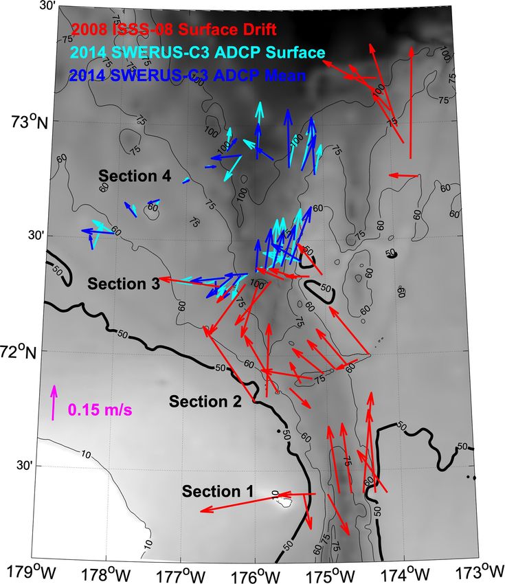
32                 J. Clement Kinney et al.: On the circulation and water mass distribution of the western Chukchi Sea

smaller than the residual current velocities. The vertical res-
olution of the LADCP data is 4 m, and the velocities were
interpolated onto the 1 m resolution of the CTD data for the
volume transport calculations.
   Geostrophic shear velocities for both cruises were com-
puted from the CTD data using the Gibbs SeaWater Oceano-
graphic Toolbox (McDougall and Barker, 2011). They were
then interpolated onto the CTD stations and the bottom tri-
angles filled assuming constant shear. To calculate absolute
geostrophic velocities, we assured that the vertical mean of
the geostrophic shear was zero and referenced to the verti-
cal mean LADCP velocity. For the two outermost stations of
each section, we used the LADCP cross-section velocities.
   No LADCP data are available for ISSS-08. Instead, we
exploited the fact that wind conditions were very calm over
the days of the ISSS-08 survey with wind speeds below
2.7 m s−1 during this period (Fig. S1 in the Supplement).
Consequently, the ship’s drift was predominantly due to sur-
face currents. An estimate of the surface currents was ob-
tained from the ship’s GPS positions during the period over
which it was drifting freely at each station. The resulting       Figure 2. Circulation pattern in Herald Canyon and refer-
ocean surface velocities were also de-tided using AOTIM           ence velocities for the geostrophic shear velocities. Shown are
(Padman and Erofeeva, 2004). The surface current speeds           2014 SWERUS-C3 vertical mean LADCP velocities (blue arrows),
obtained for ISSS-08 (0.1–0.27 m s−1 for section 3, which is      2014 SWERUS-C3 surface LADCP velocities (cyan arrows), and
common to both surveys) are consistent in magnitude with          2008 ISSS-08 surface velocities from ship drift and navigation data
the SWERUS-C3 LADCP velocities (0.03–0.25 m s−1 for               (red arrows). Bathymetry (grey-scale shading and black contours) is
surface speeds, 0.05–0.27 m s−1 for vertical mean speeds for      from the International Bathymetric Chart of the Arctic Ocean (IB-
                                                                  CAO) version 4 (Jakobsson et al., 2020).
section 3). Figure 2 shows that the ISSS-08 surface veloci-
ties for section 3 have the same pattern of northward flow in
the eastern and southward flow in the western part of Her-
ald Canyon also present in the 2014 SWERUS-C3 LADCP
observations, as well as in the 2004 and 2009 observations        fore analysis and evaluated by a six- to eight-point calibra-
presented in Linders et al. (2017). This gives us confidence      tion curve, precision being ∼ 1 %. In 2014, the same nu-
in using the surface currents derived from the ship’s drift to    trients were measured onboard using a four-channel con-
reference our geostrophic shear velocities.                       tinuous flow analyser (QuAAtro system, SEAL Analytical)
   To evaluate the robustness of the flow pattern referenc-       giving a precision between 1 % and 3 %. The quality was
ing to either vertical mean or surface currents, we referenced    assured by automatic drift control using certified reference
the geostrophic shear for the SWERUS-C3 sections to both          materials (CRM) solutions prepared from commercial am-
surface and vertical mean LADCP velocities (Fig. 2) and           poules (QC RW1, batch no. VKI-9-3-0702), except for sil-
compared them to the original ADCP velocities during the          icate where no CRM is available. During both cruises, oxy-
2014 study. Figure S2 shows that the general features of the      gen was determined using an automatic Winkler titration sys-
cross-section velocity fields are consistent between all three,   tem, giving a precision of ∼ 1 µmol kg−1 . Dissolved inor-
in particular the location of the boundary between northward      ganic carbon (DIC) was determined by a coulometric titra-
and southward flow. Volume transport computed using the           tion method based on Johnson et al. (1987), having a preci-
different velocity fields agrees closely (Fig. S3).               sion of ∼ 2 µmol kg−1 , with the accuracy set by calibration
                                                                  against CRM, supplied by A. Dickson, Scripps Institution of
2.1.2   Biogeochemistry                                           Oceanography (USA).
                                                                     The chemical variables on both cruises were sampled ev-
All chemical measurements discussed in this contribution          ery second station at 8–10 depths per station. To compute
were performed aboard the research vessels. The samples           transport of nutrients and dissolved inorganic carbon, we
were stored in cold and dark before determination, which          interpolated the bottle sample concentrations first vertically
was carried out within a day of sampling. In 2008, nutri-         onto the 1 m resolution of the CTD data and then horizontally
ents (phosphate, nitrate, and silicate) were determined by a      onto the intermediate stations. The achieved fields where
SMARTCHEM 200 discrete analyser (Westco Scientific In-            then used to compute the average concentrations of the dif-
struments/Unity Scientific). The samples were filtered be-        ferent water masses, as identified by their T − S properties.

Ocean Sci., 18, 29–49, 2022                                                              https://doi.org/10.5194/os-18-29-2022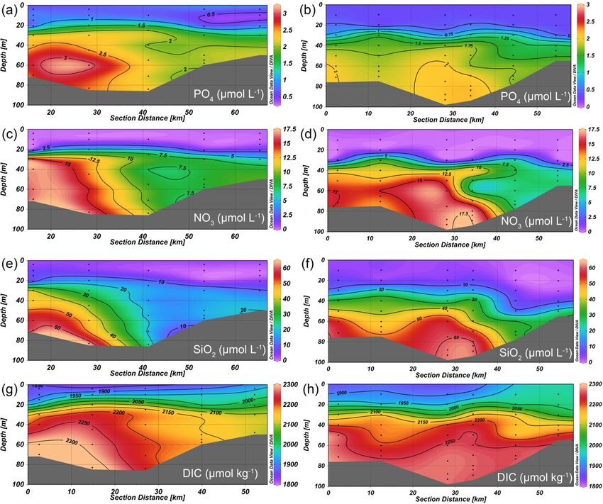
J. Clement Kinney et al.: On the circulation and water mass distribution of the western Chukchi Sea                             33

2.2    Model description

We utilize results from the Regional Arctic System
Model (RASM) to assess the circulation and water mass
characteristics in the Chukchi Sea. RASM has been devel-
oped over the past decade and each component, as well as the
fully coupled system, has been thoroughly evaluated (Brunke
et al., 2018; Cassano et al., 2017; Clement Kinney et al.,
2020; DuVivier et al., 2016; Hamman et al., 2016, 2017; Jin
et al., 2018; Roberts et al., 2015, 2018). RASM is a high-
resolution atmosphere–ice–ocean–land regional model with
a domain encompassing the entire marine cryosphere of the
Northern Hemisphere, including the major inflow and out-
flow pathways, with extensions into the North Pacific and
Atlantic oceans. RASM has been developed in order to rep-
resent Arctic relevant processes with coupling among model
components at high spatiotemporal resolution. It is a fully
coupled regional Earth system model with components in-
cluding, atmosphere, ocean, sea ice, marine biogeochem-
istry, land hydrology, and a river-routing scheme. All the
components are coupled using the flux coupler of Craig et
al. (2012). The RASM domain includes all sea-ice-covered
oceans in the Northern Hemisphere, Arctic river drainage,
and large-scale atmospheric weather patterns. The compo-
nents of RASM are the Weather Research and Forecast-
ing (WRF) atmosphere model, the Variable Infiltration Ca-
pacity (VIC) land hydrology model, and the Los Alamos
National Laboratory (LANL) Parallel Ocean Program (POP)
and Sea Ice (CICE) models. The model horizontal resolu-
tion is 50 km for WRF and VIC, and either 1/12◦ (9 km)
or 1/48◦ (2 km) for POP (ocean) and CICE (sea ice). The
RASM historical (1979–2018) simulation results analysed
here were produced after a 78-year spinup, which started
with no sea ice, and the Polar Science Center Hydrographic
Climatology (PHC) 3.0 (Steele et al., 2001) climatological
ocean temperature and salinity at rest and was forced with       Figure 3. Temperature–salinity diagrams for sections 1–4 in Her-
the Coordinated Ocean-sea ice Reference Experiments ver-         ald Canyon (section locations shown in Fig. 1b) for (a) 2008
sion 2 (CORE2) reanalysis (Large and Yeager, 2009).              and (b) 2014. Grey dots are the CTD data at 1 dB depth resolu-
                                                                 tion; coloured dots are from the bottle data colour coded by sili-
                                                                 cate concentration. Water masses are defined following Linders et
3     Results                                                    al. (2017): WW is Pacific Winter Water (this is a combination of
                                                                 remnant winter water and newly ventilated winter water shown in
In this study, we consider the dominating water masses of        Linders et al., 2017), MWR is meltwater/runoff, BSW is Bering
the Chukchi Sea: Bering Summer Water (BSW), Alaskan              Summer Water, AW is Atlantic Water, SCW is Siberian Coastal Wa-
                                                                 ter, and ACW is Alaskan Coastal Water. The bold black line marks
Coastal Water (ACW), Siberian Coastal Water (SCW), Pa-
                                                                 the surface freezing point.
cific Winter Water (WW), meltwater/runoff (MWR), and At-
lantic Water (AW). The temperature and salinity definitions
of these water masses follow Linders et al. (2017), except       ture less than −1 ◦ C and salinity above 31. BSW is warmer
that our WW is a combination of remnant winter water and         than WW with a maximum temperature of 3 ◦ C and has a
newly ventilated winter water shown in Linders et al. (2017),    salinity of 30–33.3.
and are shown in the temperature–salinity (T –S) diagrams
in Fig. 3. We focus our analysis on the WW and BSW, as           3.1   Observations of hydrography and circulation
they carry the highest nutrient concentrations, as illustrated
by silicate in Fig. 3, and contribute to the halocline of the    Section 3, at about 72◦ 200 N in the northern part of Herald
deep Arctic Ocean. We define WW as water with a tempera-         Canyon (Figs. 1b and 2), was occupied both in the begin-

https://doi.org/10.5194/os-18-29-2022                                                              Ocean Sci., 18, 29–49, 2022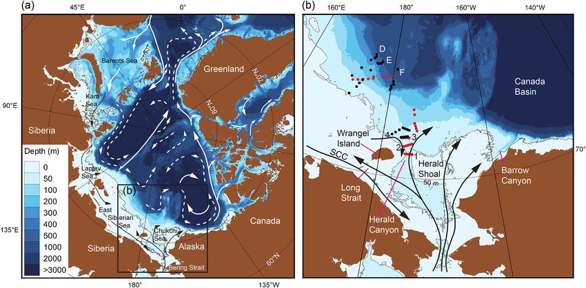
34 J. Clement Kinney et al.: On the circulation and water mass distribution of the western Chukchi Sea
Figure 4. Temperature (a, b), practical salinity (c, d) for section 3 at approximately 72◦ 200 N (Figs. 1b and 2) in 2008 (a, c, e) and
2014 (b, d, f). Panels (e) and (f) show the spatial distribution of water masses as defined following Linders et al. (2017) (see also Fig. 3)
together with cross-section velocities (m s−1 ) computed as described in section 2.2. Solid contours denote northward (positive) velocities,
while dashed ones represent southward (negative) ones. The white contours in panels (a) and (b) show the temperature structure in the WW.
Those in panels (c) and (d) are potential density σ0 (kg m−3 ).
Table 1. Mean properties of the Winter Water (WW) and Bering Summer Water (BSW) observed in 2008 and 2014.
Water mass Salinity Temp PO4 NO3 SiO2 DIC
(µmol L−1 ) (µmol L−1 ) (µmol L−1 ) (µmol kg−1 )
WW-2008 33.22 −1.55 2.46 13.5 39.1 2243
WW-2014 32.66 −1.61 1.77 11.7 40.7 2224
BSW-2008 32.25 1.12 1.49 5.1 11.3 2084
BSW-2014 32.16 0.28 1.04 4.2 10.0 2107
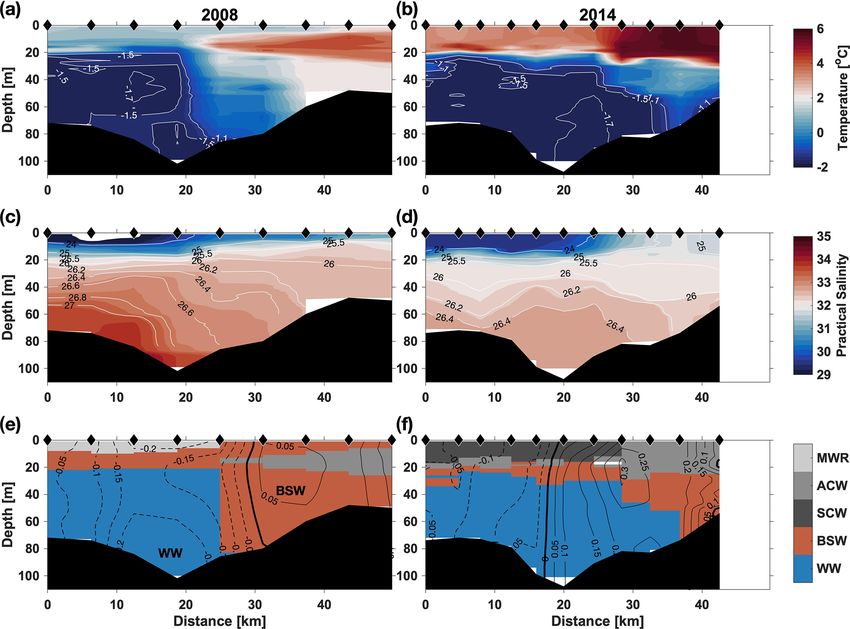
ning of September 2008 and the end of August 2014 and When comparing the T –S characteristics of the water
was used to compare the water mass characteristics, distri- masses in Herald Canyon in the 2008 and 2014 observations
bution, and circulation pattern in the two years (Fig. 4). In (Fig. 3), it is apparent that the cold WW had significantly
2008, WW dominates the western part of the canyon and lower salinities in 2014 than in 2008. The mean WW salinity
BSW its eastern part (Fig. 4e), while WW extends further in 2014 was 0.56 lower than in 2008 (Table 1). The freshen-
east in the canyon in 2014 (Fig. 4f). With salinities of 30–32 ing in the BSW is weaker (0.09 between 2008 and 2014), and
some of the shallower water with BSW characteristics in the its mean temperature shows a decrease of 0.84 ◦ C from 2008
western part of the canyon (Fig. 4) lies on the mixing line to 2014 (Table 1). This temperature change can partly be
between WW and MWR in 2008 and WW and SWC in 2014 explained by the fact that the 2008 section extends further
(Fig. 3). This water is distinctly fresher than the BSW modes east onto Herald Shoal (Fig. 1) capturing a larger part of the
that Linders et al. (2017) identify as having a Bering Strait BSW flow and partly by the fact that the freshening of the
origin and is probably of local origin. WW in 2014 has weakened the density front between BSW
Ocean Sci., 18, 29–49, 2022 https://doi.org/10.5194/os-18-29-2022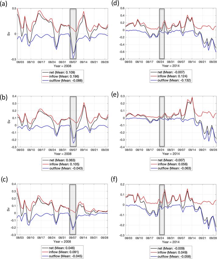
J. Clement Kinney et al.: On the circulation and water mass distribution of the western Chukchi Sea                           35

and WW leading to enhanced exchange and mixing (Fig. 4c           100 m across section 4 and dominates the total transport with
and d).                                                           a northward flow of 0.445 Sv in the mouth of Herald Canyon
    Net total volume transport across section 3 of 0.279 Sv       and a southward transport of 0.096 Sv on its western flank
(106 m3 s−1 ) southward in 2008 and 0.240 Sv northward            onto the Chukchi continental shelf. Both instances of this
in 2014 (Table 2) indicates that flow pattern and transport       WW transport contain cores with temperatures < −1.7 ◦ C in-
in this part of Herald Canyon are highly variable. Flow in        dicating recent winter ventilation (Fig. 5a).
the canyon at section 3 is pre-dominantly barotropic, south-         Our sections represent snapshots of a circulation that is
ward in the western part of the canyon and northward on           predominantly barotropic in a shallow ocean area and there-
its eastern flank (Figs. 4e, f and 5). Both surface and ver-      fore is likely strongly influenced by changes in the wind field
tical mean ADCP velocities in 2014 and surface velocities         over synoptic timescales leading to strong variability of both
from the ship’s drift in 2008 show this pattern with stronger     current pattern and strength. Furthermore, the sections do not
southward flow in the western canyon in 2008 that extends         cover the full width of Herald Canyon and thus water is also
eastward to 175.6◦ W (Fig. 4e). This results in 0.231 Sv of       flowing outside of these sections. For this reason, we com-
southward WW transport across section 3 in 2008 with a            pare the observations with model results where the sections
negligible northward component (Table 2). BSW recirculates        can be selected in suitable ways and allow us to gain an un-
southward in the centre of the canyon with a transport of         derstanding of the spatial and temporal variability of the flow
0.106 Sv southward, and a northward transport of 0.052 Sv         over a larger area and longer timescales.
at the eastern end of the section (Fig. 4e). In 2014, a west-
ward shift in the boundary between northward and south-           3.2   Modelled circulation
ward flow and the eastward extension of WW (Fig. 4f) re-
sults in a weaker southward WW transport of 0.073 Sv and a        The numerical modelling results support the general cir-
northward WW transport of 0.127 Sv in the central canyon          culation scheme of the Chukchi Sea (e.g. Brugler et al.,
that contains the core of the coldest WW with tempera-            2014) but show a more detailed picture both in time and
tures < −1.7 ◦ C (Fig. 4b and f). BSW flows predominantly         space. Mean circulation in the upper 100 m (Fig. 7a and b)
north with a net transport of 0.118 Sv (Table 2). Winds were      is similar to the schematic circulation presented in Fig. 1
southerly in the week before and including the 2014 sur-          when averaged over a 10-year period (2006–2015). Our re-
vey (Fig. 6b) and may have enhanced the flow forced by            sults show a northwestward-flowing Chukchi Slope Current,
the forward pressure coming from the Bering Strait, while         similar to recent results by Leng et al. (2021), who used
strong easterlies in 2008 (Fig. 6a) may have caused a build-      a combination of modelling and observations to examine
up of water towards Wrangel Island that potentially induced       this flow in detail. Limited observations in the Long Strait
stronger southward barotropic flow across section 3.              (Woodgate et al., 2005) suggest a northwestward flow, and
    In the southern Herald Canyon in 2008, flow across            our model results (Fig. 7) are in agreement with a long-
sections 1 and 2 was predominantly directed northward             term mean of 0.17 Sv. When we look at the circulation aver-
(Fig. 5d and e) with net total volume transport of 0.474 and      aged over a summer month when observations were collected
0.329 Sv, respectively (Table 2). Linders et al. (2017) present   (e.g. September 2008; Fig. 7c and d), we see more complex
2009 LADCP observations of northward flow across the              circulation across the shelf, as well as eddies in the Beaufort
whole canyon similar to the 2008 section 2 (Fig. 5d), sug-        Gyre. The circulation in August 2014 (during the second field
gesting that this flow pattern is not unprecedented. Conse-       expedition; Fig. 7e and f) shows much higher speeds in the
quently, section 2 has a northward WW transport of 0.198 Sv       East Siberian Sea and a weaker flow around Wrangel Island
and little southward WW flow (0.007 Sv). In section 1, very       than in September 2008. When comparing the 9 km model
little WW was observed, and its flow was thus small. The          output and the 2 km model output, there is little difference in
net northward transport of 0.474 Sv across section 1 is domi-     the long-term means, but at shorter timescales we tend to see
nated by a northward BSW transport of 0.363 Sv in the east-       higher speeds and more eddies in the 2 km simulation.
ern part of the canyon (Fig. 5e) with a smaller southward            Figure 8 shows the modelled circulation zoomed in on
component of 0.070 Sv along its western flank. The reduc-         Herald Canyon. The 10-year mean (Fig. 8a and b) shows
tion of the northward flow of BSW to 0.093 Sv at section 2        speeds of up to 10 cm s−1 northward in Herald Canyon.
and 0.052 Sv across section 3 with a recirculation of 0.106 Sv    The summer months show stronger anticyclonic flow around
in the western trough suggests there may be circulation pat-      Wrangel Island, particularly during September 2008 (Fig. 8c
terns in the trough that block the transport of BSW towards       and d), with speeds up to 12 cm s−1 north of Wrangel Island.
the Arctic Ocean. Our observations do not, however, allow         The modelled circulation also suggests that in 2014 water
us to say how often these occur or how persistent they are.       flowing northward in the eastern Herald Canyon may have
    In 2014, 0.089 Sv of BSW flows north across the eastern       been sourced from flows across the Herald Shoal (Fig. 8c–f).
part of section 4 into the Arctic Ocean (Fig. 5a and Table 2),    This may offer an explanation for higher nutrient concen-
smaller, but of a similar magnitude to the BSW transport          trations in the BSW in 2014 (Table 1). The largest differ-
across section 3. WW is found at depths between 20 and            ences between the 9 and 2 km simulations are found north of

https://doi.org/10.5194/os-18-29-2022                                                              Ocean Sci., 18, 29–49, 2022
36                    J. Clement Kinney et al.: On the circulation and water mass distribution of the western Chukchi Sea

Figure 5. Cross-section velocities in 2008 for sections from north (b, d, e) and in 2014 (a, c). Shown in all panels is geostrophic shear
referenced to the cross-section component of de-tided surface velocities from ship’s drift (2008) and LADCP (2014). The white contours
show temperature from −1 to 8 ◦ C at 1 ◦ C intervals; the green ones show temperature from −1.3 to −1.7 ◦ C at 0.2 ◦ C to highlight the
temperature structure within the WW. Please note that all sections cover different horizontal distances.

                                                                           the 100 m isobath with more complex circulation in the 2 km
                                                                           simulation.
Table 2. Volume transport computed from observations according
to section 2.2 for the sections in Herald Canyon. All transport is
in Sv (106 m3 s−1 ). Negative values denote southward transport;
                                                                           3.3   Modelled volume flux in Herald Canyon across
positive values denote northward transport. Note that the values for             section 3
the total volume transport are larger than the sum of the WW and
BSW transport due to the presence of other water masses in Herald          Next, we will examine the modelled volume transport dur-
Canyon (Fig. 3).                                                           ing August and September of 2008 and 2014, which encom-
                                                                           passes the time period when observations were collected.
 Section               1           2           3           3           4   We use the 9 km model output because it is available on a
 Latitude      71◦ 250 N   71◦ 550 N   72◦ 200 N   72◦ 250 N   72◦ 400 N
                                                                           daily timescale (instead of just monthly means in the 2 km
 Year              2008        2008        2008        2014        2014
                                                                           output), which is better for comparing with the observa-
 Net total       0.474       0.329      −0.279       0.240       0.618     tional estimates. The observed total transport across section 3
 Total north     0.572       0.390       0.082       0.357       0.745
 Total south    −0.098      −0.061      −0.361      −0.117      −0.127     was −0.279 Sv during the September 2008 occupation and
                                                                           −0.385 Sv in the model results. In 2014, the observed total
 Net WW         −0.019       0.191      −0.231       0.054       0.349
 WW north        0.004       0.198       0.000       0.127       0.445     transport was 0.240 Sv during the August occupation, while
 WW south       −0.023      −0.007      −0.231      −0.073      −0.096     the model results showed a value of −0.030 Sv. However,
 Net BSW         0.293       0.051      −0.054       0.118       0.082     time series of daily mean volume transport across section 3
 BSW north       0.363       0.093       0.052       0.132       0.089     show a large range of variability in the model results (Fig. 9).
 BSW south      −0.070      −0.042      −0.106      −0.014      −0.007     Over the 2-month period of August–September 2008 (Fig. 9),
                                                                           the net volume transport ranged from −0.4 to 0.4 Sv (nega-
                                                                           tive is southward) with a mean of 0.109 Sv. A flow reversal

Ocean Sci., 18, 29–49, 2022                                                                      https://doi.org/10.5194/os-18-29-2022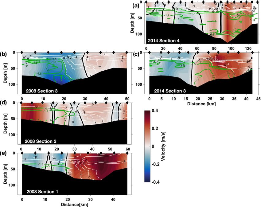
J. Clement Kinney et al.: On the circulation and water mass distribution of the western Chukchi Sea                                     37

Figure 6. Wind velocities (red vectors) and sea ice concentration (shaded) for 2007/08 and 2013/14 for (a, b) the week before and including
the CTD surveys, (c, d) an August mean for each year, (e, f) the sea ice growth season the preceding autumn (November–December mean),
and (g, h) spring conditions for each year (April–May mean).

occurred within a week’s time between 7 and 14 Septem-                  tion is required when using observations from synoptic, hy-
ber. We show vertical sections of temperature, salinity, and            drographic sections to estimate the transport of heat, fresh-
velocity on those two days for a comparison of these ex-                water, nutrients, and carbon through Herald Canyon into the
tremes (Fig. 10). The velocity core was 0.3 m s−1 southward             deep basin.
on 7 September and 0.2 m s−1 northward on 14 September.                    The amount of BSW and WW is similar during the
The model is underestimating the temperature in the upper               August–September time frames (Figs. 10 and 11) from the
layers with values only as high as 2 ◦ C, whereas the observed          model results. For example, the northward component of the
temperature (Fig. 4a) reached 4 ◦ C. The upper layer salinity           mean flow consists of 0.105 Sv of BSW and 0.091 Sv of WW
is slightly higher in the model results than in observations            during 2008. At the same time, the southward component
(Fig. 4c).                                                              of the mean flow consists of 0.043 Sv of BSW and 0.045 Sv
   Over the 2-month period of August–September 2014, the                of WW. There is more north–south variability in the time se-
net volume transport ranged between −0.5 and 0.35 Sv with               ries from 2014, as compared to 2008. The lower means re-
a mean of −0.007 Sv (Fig. 9). There was strong, persistent              flect this, with the northward component of the mean flow
southward flow during the last 10 d of September 2014, in               consisting of 0.056 Sv of BSW and 0.049 Sv of WW in 2014
contrast to the northward flow during the first half of Septem-         and the southward component consisting of 0.063 Sv of BSW
ber. Vertical sections of temperature show higher values (up            and 0.058 Sv of WW.
to 3 ◦ C) and lower salinity (< 30) in 2014 compared to 2008               Figure 12 shows the modelled monthly mean volume
(Fig. 11).                                                              transport across section 3 during 1980–2017. This gives a
   The model results allow us to place the observations at              long-term perspective of the flow through Herald Canyon
or close to events of northward (2008; Fig. 9) and south-               and indicates that the modelled mean is 0.032 Sv north-
ward (2014) net volume transport of similar magnitude (Ta-              ward for all water masses combined. This includes the
ble 2). This suggests that the model is able to realistically           northward (0.063 Sv) and southward (0.031 Sv) components.
reproduce the timing and variability of changes in circula-             BSW transport appears to be the strongest in the fall months
tion on synoptic timescales discussed above and shown in                and has been increasing in prevalence in recent years in
Figs. 10 and 11. The observed volume transport in both years            agreement with the earlier warming seen in spring in long-
is larger in magnitude and not in the same direction as the             term mooring observations in the Bering Strait (Woodgate,
modelled August–September means. This implies that cau-                 2018). The most notable feature in the time series occurred

https://doi.org/10.5194/os-18-29-2022                                                                      Ocean Sci., 18, 29–49, 2022
38                   J. Clement Kinney et al.: On the circulation and water mass distribution of the western Chukchi Sea

Figure 7. Upper 100 m averaged speed (shading) and velocity vectors (cm s−1 ) from model output. The left column (a, c, e) is from the
9 km model results and the right column (b, d, f) is from the 2 km model results. The top row (a, b) is a 10-year mean from 2006–2015.
The middle row (c, d) is a mean for September 2008. The bottom row (e, f) is a mean for August 2014. Every fourth vector for 9 km and
every 16th vector for 2 km is shown. Blue lines indicate isobaths at 25, 50, 100, and 1000 m. The red line indicates the location of section 3
discussed elsewhere. The x and y axes are labelled with model grid cell numbers.

Ocean Sci., 18, 29–49, 2022                                                                      https://doi.org/10.5194/os-18-29-2022
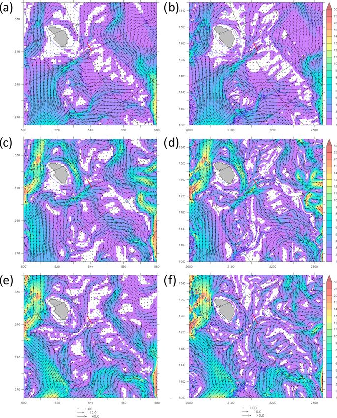
J. Clement Kinney et al.: On the circulation and water mass distribution of the western Chukchi Sea                                          39

Figure 8. Upper 100 m averaged speed (shading) and velocity vectors (cm s−1 ) from model output. The left column (a, c, e) is from the
9 km model results and the right column (b, d, f) is from the 2 km model results. The top row (a, b) is a 10-year mean from 2006–2015.
The middle row (c, d) is a mean for September 2008. The bottom row (e, f) is a mean for August 2014. Every second vector for 9 km and
every eighth vector for 2 km is shown. Blue lines indicate isobaths at 25, 50, 100, and 1000 m. The red line indicates the location of section 3
discussed elsewhere. The x and y axes are labelled with model grid cell numbers.

in November 2017, when the model showed a strong, persis-                 3.4    Nutrient concentrations and transport
tent flow reversal in Herald Canyon with southward speeds
over 30 cm s−1 (Fig. S4) averaged over the upper 100 m.                   The nutrient and DIC concentrations across section 3 in 2008
                                                                          and 2014 show the classical summer distribution of low
                                                                          values in the surface and high values in the deeper layers
                                                                          (Fig. 13). The dominating process for this pattern is primary

https://doi.org/10.5194/os-18-29-2022                                                                          Ocean Sci., 18, 29–49, 2022
40 J. Clement Kinney et al.: On the circulation and water mass distribution of the western Chukchi Sea Figure 9. Daily modelled volume flux from the 9 km simulation across section 3 during August–September 2008 for all water masses (a), BSW only (b), and WW only (c), and during August–September 2014 for all water masses (d), BSW only (e), and WW only (f). The grey box shows the time period during which observations were collected. Inflow values are northward and outflow is southward. The mean values shown are for the 2-month time period (August–September). production in the top 20–30 m, followed by sedimentation tion for each water mass was computed for the T –S ranges and mineralization at the sediment surface where the nutri- shown in Fig. 3, which avoids mean concentrations being de- ents and DIC are transported back to the bottom water. The pendent on the number of measurements. The results show highest concentrations of all properties are found more to the substantial differences in phosphate between the years, some west in 2008 than in 2014, consistent with the distribution differences in nitrate, and fairly constant silicate concentra- of WW (Fig. 4e and f). Maximum concentrations of nitrate tions (Table 1). DIC appears to be quite constant, but one and silicate were similar in 2008 and 2014, while both phos- has to consider that its concentration is high compared to phate and DIC were higher in 2008. the nutrients and also strongly salinity dependent. When the To compute the transport, the mean concentrations of nu- WW concentrations are corrected for the salinity difference, trients and DIC were calculated by first interpolating the the 2014 DIC concentration becomes 20 µmol kg−1 higher bottle sample concentrations vertically onto the T –S points than in 2008 and for the BSW the concentration becomes from the CTD reading of each station where they were avail- 31 µmol kg−1 higher. When these differences in concentra- able and, subsequently, horizontally onto the stations in be- tion are multiplied with the classical Redfield–Ketchum– tween. Using this concentration field, the mean concentra- Richards (RKR) ratios 1 : 16 : 106 for P : N : C (Redfield et Ocean Sci., 18, 29–49, 2022 https://doi.org/10.5194/os-18-29-2022
J. Clement Kinney et al.: On the circulation and water mass distribution of the western Chukchi Sea                                        41

Figure 10. Modelled vertical sections from the 9 km simulation across section 3 on 7 September 2008 (a, c, e) and 14 September 2008 (b, d, f).

al., 1963), they correspond to a shift in phosphate of 0.19 and          Table 3. Transport of nutrients and DIC on a daily basis based on the
0.30 µmol L−1 for WW and BSW, respectively, and in ni-                   measured data for the different sections; units are in 108 mol d−1 .
trate of 3.0 and 4.7 µmol L−1 for WW and BSW, respectively.              Volume transport is the total from Table 2.
These are significant differences relative to those observed
in phosphate and nitrate. Hence, from this shift in DIC, we                              Year       2008    2008      2008    2014    2014
would expect higher phosphate and nitrate concentrations                                 Section       1       2         3       3       4
in 2014 compared to 2008 in both water masses, which is op-                  Silicate    WW         −0.6      6.5     −7.8      1.9    12.3
posite to the observed. Consequently, it cannot be only local                            BSW         2.9      0.5     −0.5      1.0     0.7
biochemical processes that are responsible for the observed                  Nitrate     WW         −0.2      2.2     −2.7      0.5     3.5
differences. Most likely the source water concentrations had                             BSW         1.3      0.2     −0.2      0.4     0.3
changed, either in the properties of the water passing through
                                                                             Phosphate   WW        −0.04      0.4     −0.5     0.08     0.5
the Bering Strait, and/or differences in the contribution of                             BSW         0.4     0.07    −0.07      0.1    0.07
brine that would have a larger impact on DIC than on the nu-
trients. Utilizing the mean concentrations of Table 1 together               DIC         WW          −37      370    −448      104     671
with the volume transport of Table 2, net property transport                             BSW         528       92     −97      215     149
across the different sections and years are computed (Ta-
ble 3). Using the 37-year mean modelled volume transport
of Fig. 12, the transport of Table 3 would roughly halve for             4     Discussion
the WW and more or less vanish for BSW.
                                                                         In both observations and model, WW in 2014 was signifi-
                                                                         cantly fresher than in 2008 (Figs. 4, 10 and 11). In the ob-
                                                                         servations, it also extended further east across the canyon
                                                                         in 2014 compared to 2008 (Fig. 4). This freshening is con-

https://doi.org/10.5194/os-18-29-2022                                                                        Ocean Sci., 18, 29–49, 2022
42 J. Clement Kinney et al.: On the circulation and water mass distribution of the western Chukchi Sea Figure 11. Modelled vertical sections from the 9 km simulation across section 3 on 27 August 2014 (a, c, e) and 11 September 2014 (b, d, f). current with the large-scale freshening of the Arctic Ocean duces its density sufficiently to weaken the density front be- over recent decades, particularly in the Canada Basin (Haine tween WW and BSW across Herald Canyon potentially en- et al., 2015). Upstream observations also show that the in- hancing the exchange between the water masses (Figs. 4 flow through the Bering Strait freshened by 0.3 between 2008 and 8). and 2014 (Woodgate and Peralta-Ferriz, 2021) explaining The flow through the Bering Strait and downstream in around half of the magnitude of the observed WW fresh- the Chukchi Sea has been commonly attributed to forcing ening in Herald Canyon (Table 1). In addition, we suggest by the local winds and a far-field difference in sea surface that variability in the wind field and circulation the previ- height (SSH) between the Pacific and Arctic, or so-called ous winter over the East Siberian and western Chukchi shelf “pressure head” (Coachman and Aagaard, 1966; Stigebrandt, may have enhanced the upstream freshening signal. Winds 1984). A more recent study (Peralta-Ferriz and Woodgate, over the Chukchi Sea are generally northeasterly in win- 2017) based on the GRACE ocean mass satellite data and ter, piling water against the Siberian coast and preventing in situ mooring data suggests the dominant role of the East its northward flow until they weaken in spring (Pickart et Siberian Sea (ESS) in driving the flow through the Bering al., 2010). This pattern is clearly apparent in winter and Strait. Their analysis shows westward winds driving north- spring 2007/08 with strong northeasterlies in November and ward Ekman transport of shelf waters into the basin, which December 2008 and weaker easterlies in April and May 2008 lowers SSH in the ESS and amplifies the pressure head forc- (Fig. 6e and g). Winds in winter and spring 2013/14 were ing. While the measurements are very limited, the north- weaker than in 2007/08 and southwesterly (Fig. 6f and h). westward flow toward the Long Strait originates in the west- This may have reduced the residence time on the shelf lead- ern side of the Bering Strait and is most likely (Woodgate ing to a reduced salinity enhancement of the shelf waters due et al., 2005) steered toward the Long Strait by the shallow to brine release during sea ice formation, but also to a larger bathymetry gradients, westward winds, and the SSH gradi- volume of fresher WW being formed in winter 2013/14. The ent centred at one end on the ESS. Note that the coastal cur- observed (and modelled) freshening of the WW in 2014 re- rent that flows southeastward in the southwestern Chukchi Ocean Sci., 18, 29–49, 2022 https://doi.org/10.5194/os-18-29-2022
J. Clement Kinney et al.: On the circulation and water mass distribution of the western Chukchi Sea                            43

                                                                      Modelled volume transport showed a large range of vari-
                                                                   ability in Herald Canyon on a daily timescale (Fig. 9).
                                                                   Flow reversals were common and occurred during August–
                                                                   September of both 2008 and 2014. This is consistent with
                                                                   observational data from 1990–1991 in Herald Canyon, which
                                                                   showed flow reversals lasting a week or more that were cor-
                                                                   related with the wind field (Woodgate et al., 2005). Synop-
                                                                   tic storms enter the Chukchi Sea frequently during the late
                                                                   summer/fall time period and are a driving force for the flow
                                                                   in Herald Canyon (Pickart et al., 2010). The ocean compo-
                                                                   nent of RASM is coupled to a relatively high-resolution at-
                                                                   mospheric component within the system model; however, er-
                                                                   rors in the representation of atmospheric fields would likely
                                                                   be in the direction of underrepresentation of the strength of
                                                                   storms. This leads us to conclude that the large variability in
                                                                   modelled flow is valid and that short-term measurements of
                                                                   the speed and direction of the flow are not necessarily repre-
                                                                   sentative of the mean over time.
                                                                      The currents computed from the observations, as well as
                                                                   the numerical modelling results, show southward-flowing
                                                                   water in the western Herald Canyon (Figs. 4 and 8). This
                                                                   southward-flowing water most likely has the East Siberian
                                                                   Sea as a source, which is supported by the hydrographic sig-
                                                                   nature of the water as well as the general circulation from
                                                                   the model results (Fig. 8). It has high nutrient concentra-
                                                                   tions, typical for decay of organic matter, but not high enough
                                                                   salinity to come from any substantial depth along the conti-
                                                                   nental margin (Fig. 14a). Also, its temperatures are close to
                                                                   the freezing point, significantly lower than the temperature of
                                                                   water at the shelf break with the same high silicate concentra-
                                                                   tion (Fig. 14b). Furthermore, it has a higher oxygen concen-
                                                                   tration than the slope water at the high silicate concentration
                                                                   (> 40 µmol L−1 ), as exemplified by the 2014 data in Fig. 14c.
                                                                   The only exception is the deepest water in the northern sec-
                                                                   tion, with silicate concentrations above 70 µmol L−1 ; water
                                                                   that most likely includes some intrusions of the slope current
                                                                   as it also has higher salinity and temperature compared to
                                                                   the WW.
                                                                      Winsor and Björk (2000) used a polynya model driven
Figure 12. Monthly mean modelled volume flux (Sv) from the
                                                                   by atmospheric forcing to compute ice, salt, and dense wa-
9 km simulation across section 3 during 1980–2017 for all water
masses (a), BSW only (b), and WW only (c). Inflow values are
                                                                   ter production in different regions of the Arctic Ocean over
northward and outflow is southward.                                39 winter seasons from 1958 to 1997. The area west of
                                                                   Wrangel Island was one region where many polynyas formed
                                                                   and created high-salinity waters from brine produced by ice
Sea (the Siberian Coastal Current – SCC) is seasonal and           formation.
it has been observed only during some years (Weingartner              Another aspect is the fate of the southward-flowing water
et al., 1999). The model does show a similar southeastward         to the western Herald Canyon; is it recirculating within Her-
flow (SCC) sometimes and at shorter timescales. However,           ald Canyon or is it flowing around Wrangel Island back into
the long-term mean flow is to the northwest through the Long       the East Siberian Sea? Our observational data cannot reveal
Strait. This flow in the mean model results follows the topo-      this, but as most of the high-nutrient water is deeper than
graphic constraints of the Siberian coast and is a result of the   50 m, a depth that to our knowledge exceeds that south of
predominant westward winds and pressure head forcing, in           Wrangel Island; the most plausible conclusion is a recircula-
agreement with the cited literature. Its seasonal and interan-     tion in the canyon. Also, there are some indications of two
nual variability are driven by the combination of these two        cores of high-nutrient water in 2014 at section 3, one in the
factors.                                                           west on the shallower part and one in the deep central canyon

https://doi.org/10.5194/os-18-29-2022                                                               Ocean Sci., 18, 29–49, 2022
44 J. Clement Kinney et al.: On the circulation and water mass distribution of the western Chukchi Sea Figure 13. Observed nutrient and DIC sections at latitude about 72◦ 200 N (noted as 3 in Fig. 1b) in 2008 (a, c, e, g) and 2014 (b, d, f, h). (Fig. 13b, d and f), that could be a result of one south- and nitrate flux and 2.4×10¹² mol C yr−1 (28×1012 g C yr−1 ) us- one north-flowing core. ing the phosphate flux, all based on the RKR ratios. However, When assuming that the southward-flowing water recircu- these numbers have to be taken with care as the model an- lates in Herald Canyon it also means that the net flux gives nual average volume transport of BSW and WW in section 3 the total transport within the geographic range of the sec- was only 15 % of the computed from the measured proper- tion, i.e. if the water that recirculates is included in the north- ties. It is evident, though, that nitrate is the limiting element flowing current. Hence, the transport of Table 3 represents and that a volume transport of 0.431 Sv (Table 1) makes a snapshots of the supply to the north. It should be noted that major contribution to the fuelling of primary production in this section does not cover all waters that flow either to the this region of the Arctic Ocean. For instance, Anderson et south or to the north and thus comes with substantial uncer- al. (2003) used the phosphate deficit in the central Arctic tainties. However, Fig. 5a suggests that more of the north- Ocean to compute an export production that corresponded ward flow is missed, which indicate that the transport is un- to 2.5 × 10¹² g C yr−1 of the Canadian Basin photic zone; derestimated. The supply of nutrients contributing to new i.e. the supply by the BSW and WW could contribute 5 times primary production in the central Arctic Ocean in 2014 can this export if it reached the photic zone. However, this is not be computed from the transport in section 4 (Table 3), the expected, at least not under the present oceanographic con- most northerly and thus the one that might best represent the ditions, but points to the importance of the transport through flux into the deep basins. Adding together the transport in the the Herald Canyon as a source of nutrients to the central Arc- BSW and WW, we achieve a potential new primary produc- tic Ocean. High values of primary production were also mod- tion of 0.9 × 10¹² mol C yr−1 (11 × 1012 g C yr−1 ) using the elled in the Long Strait and much of the East Siberian Sea Ocean Sci., 18, 29–49, 2022 https://doi.org/10.5194/os-18-29-2022
J. Clement Kinney et al.: On the circulation and water mass distribution of the western Chukchi Sea                              45

Figure 14. Plots of SWERUS-C3 East Siberian Sea shelf-break data compared with those of Herald Canyon: silicate versus salinity (a),
silicate versus temperature (b), and oxygen versus silicate (c). Locations of the stations are noted in the map of Fig. 1b.

during June 2011 (Clement Kinney et al., 2020), apparently          gave a transport to the north of 0.24 Sv of which ∼ 20 %
driven by a northwestward flow through the Long Strait. The         was WW and ∼ 50 % was BSW, with the remaining ∼ 30 %
arrival of high-nutrient water from the western side of the         being surface waters. This large variability in transport, in-
Bering Strait when combined with accelerated early sea ice          cluding a change in the direction, points to the flow in Her-
melt created conditions that were favourable to primary pro-        ald Canyon being highly variable in time and space, a result
duction in the East Siberian Sea.                                   of the shallow water environment being sensitive to the wind
                                                                    and sea ice conditions. This is also illustrated by the simu-
                                                                    lated daily modelled net volume transport for the same sec-
5   Conclusions                                                     tion that ranged from −0.4 to 0.4 Sv (negative is southward)
                                                                    with a mean of 0.109 Sv over the 2-month period of August–
Numerical modelling results show that a substantial frac-           September 2008, while it ranged between −0.5 and 0.35 Sv
tion of Pacific Water that enters the Chukchi Sea through           with a mean of −0.007 Sv for the same months in 2014. A
the Bering Strait continues into the East Siberian Sea via          long-term perspective for the period 1980–2017 indicates a
the Long Strait south of Wrangel Island. Both the model re-         modelled mean transport of 0.032 Sv northward for all water
sults and hydrographic conditions support that some of this         masses combined, which includes a northward component
water flows north of Wrangel Island back into the Chukchi           of 0.063 Sv and a southward of 0.031 Sv. However, the maxi-
Sea and is entrained in the northward-flowing water of Her-         mum monthly transport is up to 0.2 Sv to the north and nearly
ald Canyon that supplies the halocline of the central Arctic        as much to the south. The BSW transport has a relatively ev-
Ocean. The net transport in Herald Canyon, at a section lo-         ident seasonal signal with the strongest transport in the fall
cated about 72◦ 200 N, was computed based on observations           months, also with a tendency for increasing transport during
in September 2008 to be about 0.3 Sv to the South, of which         the last decade. The WW transport on the other hand does
∼ 80 % had WW properties, while ∼ 20 % was BSW. In Au-              not show any seasonal pattern.
gust 2014, on the other hand, corresponding computations

https://doi.org/10.5194/os-18-29-2022                                                                Ocean Sci., 18, 29–49, 2022
You can also read