Comparing 3D Point Cloud Data from Laser Scanning and Digital Aerial Photogrammetry for Height Estimation of Small Trees and Other Vegetation in a ...
←
→
Page content transcription
If your browser does not render page correctly, please read the page content below
remote sensing
Article
Comparing 3D Point Cloud Data from Laser Scanning and
Digital Aerial Photogrammetry for Height Estimation of Small
Trees and Other Vegetation in a Boreal–Alpine Ecotone
Erik Næsset * , Terje Gobakken                    , Marie-Claude Jutras-Perreault and Eirik Næsset Ramtvedt

                                          Faculty of Environmental Sciences and Natural Resource Management, Norwegian University of Life Sciences,
                                          P.O. Box 5003, 1432 Ås, Norway; terje.gobakken@nmbu.no (T.G.);
                                          marie.claude.jutras.perreault@nmbu.no (M.-C.J.-P.); eirik.nasset.ramtvedt@nmbu.no (E.N.R.)
                                          * Correspondence: erik.naesset@nmbu.no

                                          Abstract: Changes in vegetation height in the boreal-alpine ecotone are expected over the coming
                                          decades due to climate change. Previous studies have shown that subtle changes in vegetation height
                                          (
Remote Sens. 2021, 13, 2469                                                                                             2 of 31

                              is reduced. Migration of the alpine and northern tree lines will influence future carbon
                              pools. A need therefore exists to monitor vegetation changes in these areas [8].
                                     Airborne laser scanning (ALS) has been proposed as a technique to monitor subtle
                              changes near the tree lines, such as colonization of treeless areas [9], to assist in prediction
                              and estimation of tree height [9–11], and to estimate subtle changes in tree and vegetation
                              height [12]. Numerous studies [9,11,13–18] have shown that ALS data with point densities
                              of 7–11 points m−2 may be applied to detect individual pioneer trees in the alpine tree line.
                              With such pulse densities, about 90–100% of the trees with heights greater than 1 m are
                              likely to be hit by laser pulses resulting in echoes with height values greater than zero,
                              i.e., located above the terrain surface. Echoes with heights >1 m are mainly tree echoes.
                              However, because laser beams of pulse lasers will tend to penetrate into the canopies
                              before an echo is triggered, even the maximum of the recorded echo heights will typically
                              underestimate the height of small trees. For example, Ref. [9] reported an underestimation
                              of tree height by 0.43 m to 1.01 m, depending on tree species and tree height. The tree
                              heights in their dataset ranged from 0.11 m to 5.20 m, which implies that the smaller trees
                              will tend to have recorded laser echoes with height values equal to zero even when a tree
                              is hit by a laser pulse. This will limit the sensitivity of ALS as a tool for early detection of
                              recently established trees.
                                     Three-dimensional (3D) photogrammetric point data produced in digital aerial pho-
                              togrammetry (DAP) from imagery acquired by aircraft and unmanned aerial systems (UAS)
                              have in recent years become a viable alternative to 3D data from ALS in forest and vegeta-
                              tion studies. DAP is an alternative to ALS in, for example, operational inventory of forest
                              resources (e.g., [19,20]), although with somewhat lower accuracy than by use of ALS [21],
                              but still economically competitive to ALS in forest inventory when both cost and utility
                              of the data are taken into account [22]. 3D data from DAP based on UAS imagery have
                              shown great promise in terms of precision of estimates of parameters such as volume and
                              biomass in different forest types – from boreal forests ([23]) to dry African savannah [24].
                                     It is usually cheaper to acquire 3D data from DAP than from ALS and UAS offer
                              greater flexibility for small areas than acquisition from larger airborne platforms. Use
                              of 3D data extracted by DAP from imagery acquired by UAS may therefore be a viable
                              option to assist in detection and estimation of height of small trees in smaller areas in the
                              forest–alpine or forest–tundra ecotones. Further, because a passive sensing technique like
                              optical imaging may better capture the properties on the outer surface of a tree canopy than
                              lasers, which tend to penetrate the canopy, DAP may in fact offer additional advantages
                              compared to ALS for tree detection and estimation of height [19].
                                     Still, to our knowledge, there is no scientific evidence of the performance of 3D data
                              from DAP for small tree detection and height estimation in the forest–alpine or forest–
                              tundra ecotones. A recent study by Ref. [25] may, however, give an interesting perspective
                              on the potential usefulness of 3D data from UAS DAP for estimation of properties of small
                              trees. Ref. [25] estimated mean tree height using DAP from imagery acquired with UAS
                              over young forest stands under regeneration. The mean plot and stand height in their
                              dataset ranged from 0.5 m to 13.0 m with an average value of 2.5 m. They found that
                              the RMSE of the mean height estimate produced with assistance of 3D DAP data was
                              substantially smaller than obtained with ALS. Although this study only addressed mean
                              values of groups of trees (plots, stands) rather than individual trees, their findings may
                              suggest that DAP also may be useful to assist in quantifying properties of individual small
                              trees. In an assessment of UAS 3D point clouds from laser and DAP for individual tree
                              height estimation over tree plantations with an average tree height of 2.6 m, Ref. [26]
                              reported that DAP underestimated height to a greater extent than laser and that the
                              accuracy was greater for laser than for DAP. However, their 3D data had an exceptionally
                              high point density (443–939 points m−2 for DAP and 325–649 points m−2 for laser), which
                              makes comparisons with previous findings based on data from airborne platforms and
                              coarser resolution imagery difficult.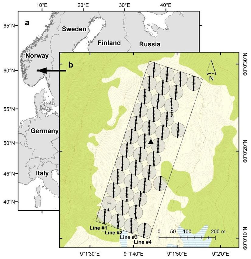
Remote Sens. 2021, 13, 2469                                                                                            3 of 31

                                    There are currently no commercial interests associated with small trees and other
                              vegetation in the tree line ecotones, as there are in the productive forests where small
                              trees represent young forest in an early stage of a rotation after clear-felling (cf. [25,26]).
                              The primary purposes of quantifying and monitoring small trees and other vegetation
                              in the tree line ecotones is therefore partly to keep track of how climate change affects
                              this climate sensitive ecological environment and to enable consistent analysis of the net
                              climate feedback of tree line migration caused by changes in biomass and soil carbon pools
                              and changes in albedo. Ref. [12] proposed several statistical estimators to estimate changes
                              in height of trees and other vegetation using bi-temporal data from ALS in a boreal-alpine
                              ecotone. The estimators were applied to an observation period of six years and it was
                              demonstrated that statistically significant increases in height could be found for relatively
                              small monitoring units (1.5 ha primary monitoring units). The estimation framework was
                              proposed as an operational methodology that could be applied to monitoring over vast
                              tracts of land, and it was based on a so-called model-dependent approach to statistical
                              inference. The method relies on bi-temporal 3D data from remote sensing and temporally
                              consistent ground observations of heights of trees and other vegetation. Because the
                              precision (confidence interval) of the height change estimates will determine the sensitivity
                              of the method to detect subtle changes in height, it is important to quantify to what extent
                              the source of the 3D information (ALS vs. DAP) influence the precision of the estimates.
                                    The current study focused on the boreal-alpine ecotone in particular. The objectives
                              were twofold. (1) We assessed and compared the performance of 3D data from ALS and
                              DAP for prediction of tree height of small pioneer trees and evaluated how tree size and
                              tree species affected the predictive ability of the two types of 3D data. (2) We compared the
                              precision of vegetation height estimates (trees and other vegetation) across the chosen study
                              area using 3D data from ALS and from DAP using the estimators proposed by Ref. [12].
                              As part of the latter objective, we also evaluated the different sources of uncertainty in the
                              model-dependent mean square error estimators for vegetation height at different spatial
                              scales. It should be noted that this analysis focused on height estimation rather than height
                              change estimation because 3D data from DAP to be compared with ALS data were available
                              just for one point in time. An operational methodology for change estimation could indeed
                              exploit combined bi-temporal ALS and DAP data, but we wanted to quantify the effect of
                              each of them on the precision of estimates without confounding the effects of the two 3D
                              acquisition techniques.

                              2. Materials and Methods
                              2.1. Study Area
                                    The study area is located in the municipality of Rollag in southern Norway (60◦ 00 N
                              9◦ 010 E, 910–950 m above sea level) (Figure 1). The entire study was conducted within
                              a 200 m × 600 m rectangle (12 ha). The work took place in the boreal–alpine tree line,
                              which at this location was around 900–940 m above sea level. The main tree species in the
                              trial area are Norway spruce (Picea abies (L.) Karst.), Scots pine (Pinus sylvestris L.), and
                              mountain birch (Betula pubescens ssp. czerepanovii). The total stem density when the study
                              area was established in 2006 was estimated to be 97 trees ha−1 , of which only 15 trees ha−1
                              were taller than 2 m [9].

                              2.2. Field Measurements
                              2.2.1. Overview
                                   This study comprised field data from two complementary datasets which both have
                              been subject to analysis in previously published work but updated with new and original
                              measurements for the purpose of the current study.
                                   First, we selected and georeferenced individual trees that could be used as ground-
                              reference (1) for analysis of various types of remotely sensed data and the performance
                              of such remotely sensed data to identify individual pioneer trees; (2) for detection of
                              subtle changes at tree level over time using remotely sensed data; and (3) for development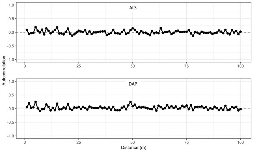
Remote Sens. 2021, 13, 2469 4 of 31
of methods for operational monitoring of vegetation changes over time by assistance of
remotely sensed data, which subsequently could be adapted to monitoring over vast tracks
of land. (4) An overarching purpose was to establish a long time series of individual tree
data that could be used as reference for biological studies of changes in the tree cover in
the boreal-alpine ecotone caused by anthropological drivers of change. The time series was
established in 2006 and is still maintained, see details in Section 2.2.2. The individual tree
dataset was subject to analysis under objectives #1 and #2.
Second, ALS data have to date been the primary source of remotely sensed data
under study of pioneer trees. Because the sensitivity of ALS data for early detection of
emerging pioneer trees depends on the accuracy of the digital terrain model (DTM) used
for normalization of the ALS vegetation echoes, we collected ground reference points with
known elevation and ground properties (e.g., terrain form and type of ground vegetation;
see details in Section 2.2.3). The primary purpose was to assess systematic errors and
accuracy of DTMs constructed from ALS data under different acquisition strategies, such
as flying altitudes and pulse repetition frequencies. This dataset also contained valuable
information on other vegetation than trees which complemented the individual tree dataset.
It was subject to analysis under objective #2.
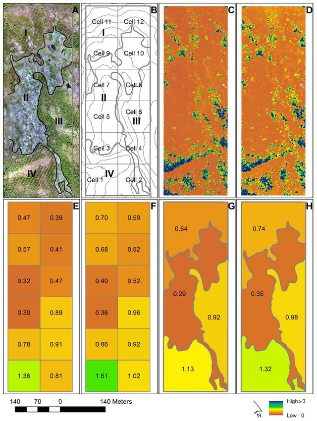
Figure 1. (a) Location of the study area and (b) design of the trial. Black dots are the ground reference
points (n = 426); small circles indicate the locations of the point-centered quarter sampling points
(black dots; n = 40), which were centers of the 25 m radius plots (gray circles) arranged along four
sample lines; green is defined as forest according to the official N50 topographic map series; light
yellow is above the tree line; the black triangle is the reference point (base station).
2.2.2. Individual Tree Data
The individual tree dataset was established in 2006 [9] and re-measured in 2012 [12]
and 2017. In 2006, the point-centered quarter sampling method (PCQ; [27]) was used to
select individual trees for the study. The tree sampling was conducted according to PCQ at
40 systematically distributed sample points within the 200 m × 600 m rectangle (Figure 1).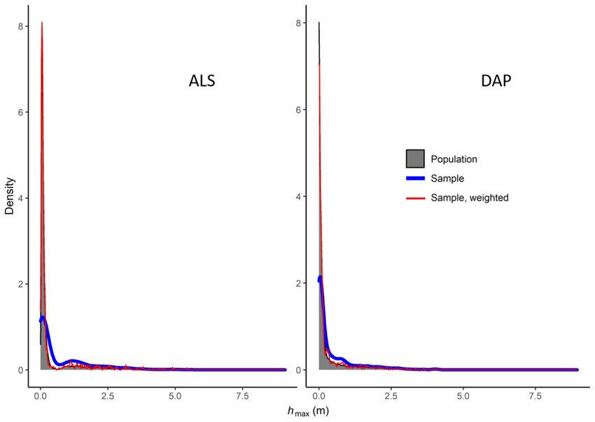
Remote Sens. 2021, 13, 2469                                                                                                     5 of 31

                              It should be noted that due to time constraints, only four points were measured on line #4,
                              see Figure 1.
                                   At each point, the closest tree in each of four height classes (3 m)
                              within each of the four quadrants around the points defined according to the cardinal
                              directions, i.e., the NE, SE, SW, and NW quadrants, was selected. Thus, a maximum of
                              16 trees were selected at each point. It should be noted that the selection of trees was
                              restricted to a maximum distance from each sample point of 25 m [28].
                                   The stem positions of the trees were recorded with a real-time differential global
                              positioning system (GPS) and global navigation satellite system (GLONASS) receiver,
                              with a local reference receiver for differential correction located within the study area
                              (Figure 1) at a national reference point of the Norwegian Mapping Authority. The expected
                              accuracy was 3–4 cm [9]. For each tree, tree species, tree height, stem diameter at root
                              collar, and crown diameter in two perpendicular directions (N–S and E–W) were recorded.
                              In total, 342 trees were selected, ranging from 0.11 to 5.20 m in height. Details regarding
                              the field work in 2006 can be found in Ref. [9]. The trees took many different forms,
                              including distinct and solitary trees, groups of trees—for spruce often as krumholtz, and
                              birch appearing as solitary trees as well as in the form of tall scrubby vegetation (Figure 2).

                              Figure 2. Tree measurements during field work in 2006 (A,B) and measurements of ground reference
                              points in 2010 (C,D,E). (A) Spruce tree appearing in a group of trees. (B) Birch tree part of a group of
                              trees forming tall scrubby vegetation. (C) Ground reference point with vegetation height > 0.20 m
                              and “green vegetation”. (D) Ground reference point with vegetation height 0.10–0.20 m and “green
                              vegetation”. (E) Ground reference point with vegetation height < 0.10 m and “rock/bare” surface.

                                   When the field work was repeated in 2012 and subsequently in 2017, the already
                              defined 40 sample points were once again identified with real-time GPS + GLONASS.
                              For each of the 40 points, the PCQ sampling was then conducted independently of the
                              sampling in 2006, but according to the same protocol. Many of the trees selected in 2012
                              and 2017 were the same as those measured in 2006. During the 2017 campaign, which
                              took place in the period 8 August to 21 September, we identified all trees that had been
                              measured in 2006 and 2012 [12] and which were still alive, including those that were not
Remote Sens. 2021, 13, 2469 6 of 31
selected for the 2017 PCQ sample. Thus, for the current study, we measured and analyzed
all trees selected into the 2017 PCQ sample in addition to trees measured in 2006 and 2012
and which were alive in 2017. The individual tree recordings in 2017 followed the same
protocol as in 2006. In total, 532 trees were recorded, ranging between 0.05 and 6.60 m in
height (Table 1). The field-recorded heights of the trees were designated h. The 2017 data
have not been published before.
Table 1. Summary of field measurements of 532 trees recorded in 2017.
Tree Species Characteristic n Range Mean
Tree height (m) 236 0.05–6.60 1.46
Norway spruce
Crown area a (m2 ) 236 0.0003–23.378 2.507
Tree height (m) 90 0.05–3.00 0.53
Scots pine
Crown area a (m2 ) 90 0.0007–2.114 0.241
Tree height (m) 206 0.11–4.00 1.51
Mountain birch
Crown area a (m2 ) 206 0.0012–9.726 1.756
Tree height (m) 532 0.05–6.60 1.32
All trees
Crown area a (m2 ) 532 0.0003–23.378 1.83
a Crown area calculated as the area of an ellipse with the perpendicular crown diameter measurements as axes.
2.2.3. Ground Reference Points
The ground reference point (GRP) dataset was acquired in August 2010 [29]. A total
of 440 GRPs were distributed at 5 m intervals in the N-S direction through the center
points of the 40 PCQ plots using a measuring tape and a hand-held compass. Real-time
GPS + GLONASS was used to record the coordinates of each GRP. For some points the
positioning was unreliable due to poor radio link between the base and rover receivers.
Thus, 426 of the initial 440 points were available for analysis (Figure 1). For each GRP,
three variables were recorded. They were “terrain form”, “terrain surface”, and “veg-
etation height”. Vegetation height was recorded according to three mutually exclusive
height classes, namely 0.20 m. Terrain surface was recorded
according to three mutually exclusive classes, namely “rock/bare”, “lichen/heather”,
and “green vegetation”. Heather comprised common heather (Calluna vulgaris), crowberry
(Empetrum nigrum L.), cowberry (Vaccinium vitis-idaea), mountain heath (Phyllodoce caerulea),
and alpine azalea (Loiseleuria procumbens), but not bilberry (Vaccinium myrtillus L.). The
latter was classified as green vegetation.
In the analysis addressing objective #2, a model-dependent approach to inference was
adopted, by which the height of trees and other vegetation was estimated for various do-
mains of the study area. Under model-dependent inference, approximate unbiasedness of
the estimators can only be assured if the model used for prediction is correctly specified for
the domain of application. Since the vegetation in the study area is a mix of scattered trees
of different species and other vegetation, the tree dataset alone would probably not warrant
appropriate models for prediction of height of all vegetation, see detailed discussion in
Ref. [12]. The GRPs with recorded vegetation height were considered complementary to
the tree data for combined modelling of vegetation height for all vegetation, trees included.
Since the vegetation height was recorded in ordered classes only, we assigned a height
value of 0.05 m to GRPs in the class 0.20 m, GRPs with vegetation height >0.20 m
were discarded. In some cases, trees actually constituted the vegetation cover for points
with height >0.20 m (see example in Figure 2C). Among the 426 recorded GRPs, 365 were
subject to further analysis (Table 2). In a similar way as for the trees, the vegetation height
for the GRPs was designated h.Remote Sens. 2021, 13, 2469 7 of 31
Table 2. Frequency distribution of 365 ground reference points recorded in 2010.
Terrain Surface
Vegetation Height Rock/Bare Lichen/Heather Green
0–0.10 m 17 37 251
0.10–0.20 m 0 0 60
2.3. Laser Scanner Data
ALS data were acquired under leaf-on conditions using a fixed-wing aircraft. The
acquisition took place on 18 June 2017 using a LMS-Q1560 laser scanner system (Riegel,
Horn, Austria) and was part of the governmental effort to construct a new detailed terrain
model for Norway. The study area was located within a 1169 km2 ALS block for which
ground control points were established across the entire block for calibration of the height
of the laser measurements. The contracted minimum point density for the block expressed
as number of first echoes per 10 m × 10 m cell tessellating the block was 5 points m−2 .
The data satisfied this criterion within our study area. In fact, in certain parts of the 12 ha
study area the point density was >25 points m−2 due to side overlap between adjacent,
parallel strips and a single flight line perpendicular to the main direction of the scanned
block. This dataset was used by the data vendor (TerraTec, Oslo, Norway) to produce the
official national terrain model by classifying the points as ground and non-ground echoes
using the progressive triangular irregular network (TIN) densification algorithm [30] in the
TerraScan software [31].
The official national terrain model was used as terrain reference surface for the study.
However, a harmonization of the point density was considered important because order
statistics were used in the analysis of the tree and vegetation height. Order statistics, such
as maximum height, are monotone increasing functions of number of points for a given
target area [32]. In order to keep the point density stable across the study area, we discarded
all data from the perpendicular flight line and from the overlap zone between adjacent,
parallel strips. The resulting mean point density across the 12 ha area was reduced to
6.5 points m−2 for “first” and “single” echoes.
Normalized height values were computed for all “first” and “single” echoes relative
to the official TIN by linear interpolation. Only “first” and “single” echoes with normalized
height values were used in the subsequent analysis. All classified ground and non-ground
points with negative normalized height values were assigned the value zero. All classified
ground points were assumed to lie on the official terrain surface and where therefore
assigned the value zero.
2.4. Unmanned Aerial Systems Image Data
UAS image data were acquired under leaf-on conditions using a eBee fixed-wing
drone (senseFly Ltd, Cheseaux-Lausanne, Switzerland) weighing approximately 0.41 kg
without payload [33]. The acquisition took place on 21 June 2017, three days after the
ALS acquisition, using a Canon IXUS127 HS (Canon Inc., Tokyo, Japan) red, green, and
blue camera producing three separate 16.1 megapixel images in the red (660 nm), green
(520 nm), and blue (450 nm) wavelengths. The drone was equipped with an inertial
measurement unit and an on-board Global Navigation Satellite System (GNSS) to control
the flight parameters and provide rough positioning during flight operations [33]. The
eBee flight plan was managed through senseFly’s eMotion 2 software, ver. 2 [33], installed
on a laptop computer. The longitudinal and lateral image overlaps were set to 90% and
80% respectively, although only a longitudinal overlap of 70% was achieved during the
survey. The ground pixel resolution was set to 3.9 cm.
Prior to the image acquisition, the position of ten ground control points (GCPs)
were determined and measured using the same RTK-based procedure as the one used
to record positions of the GRPs. The GCP targets consisted of a set of 1 × 1 cross-Remote Sens. 2021, 13, 2469 8 of 31
shaped 4 cm × 46 cm timber planks painted orange to insure good contrast with the
background vegetation.
The UAS images were processed in Agisoft PhotoScan Professional software, ver. 1.4.3
(Agisoft LLC, St.Petersburg, Russia), to produce a 3D point cloud [34]. The processing
steps followed in the PhotoScan software together with the parameters used are described
in Table 3.
Table 3. Processing steps with corresponding parameters in Agisoft PhotoScan Professional software
for the generation of 3D point cloud from UAS imagery.
Task Parameter
Alignment Accuracy: high a
Generic preselection: yes a
Reference preselection: yes a
Key point limit: 40,000 a
Tie point limit: 4000 a
Adaptative camera model fitting: yes a
Guided marker positioning Number of GCPs: 10
Depth maps and dense point cloud Quality: medium b
Depth filtering: mild b
a Parameters suggested in PhotoScan online tutorial [35]. b Parameters chosen using a trial and error approach.
After initial testing, an adaptive camera model fitting was used to perform the align-
ment. This function automatically selects the camera parameters to be included in the
adjustment based on their reliability. The position of the GCPs were imported in the soft-
ware to improve the estimates of the camera position and orientation. The GCP positions
were manually refined and the camera alignment was optimized based on the GCPs to
allow a more accurate model reconstruction. The average RMSEs associated with the
estimated camera and GCP locations compared to the PhotoScan-estimated values were
0.92 m and 0.06 m, respectively. A dense point cloud was constructed using a medium
quality parameter to reduce excessive processing time and a mild depth filtering parameter
to remove outliers and reduce noise while allowing height variation between the 3D points.
The point density of the resulting dense point cloud was around 50 points m−2 .
At this point we would like to clarify that the DAP methodology applied in this
study is what is commonly known in the literature as structure-from-motion (SfM). Using
an iterative least-squares solution, camera position and orientation, and scene geometry
are simultaneously reconstructed by identification of matching features, or tie points, in
multiple images. The output from SfM is fixed into a relative, not absolute, coordinate
system [36]. The GCPs were used to transform the data to the absolute coordinate system
adopted in this study. For the sake of simplicity, we refer to this methodology as DAP.
Normalized height values were computed for the DAP points relative to the official
TIN by linear interpolation. Because the absolute height values of the DAP data were
determined according to the elevation of the ten GCPs, we compared the elevation of
the GCPs to the elevation of the official TIN. There was a mean difference in elevation
of 0.055 m with a standard deviation of the differences of 0.028 m. The mean difference
was subtracted from the normalized heights of all the DAP points. All DAP points with
negative normalized height values after this subtraction were assigned the value zero.
2.5. Extracion of ALS Data and DAP Data for Trees, Ground Reference Points, and
Population Elements
2.5.1. Trees
Crown polygons for the recorded individual trees were constructed as ellipses around
the recorded stem positions with the perpendicular crown diameter measurements (N–S,
E–W) as minor and major axes. The tree crown polygons were laid atop the ALS dataset
and the DAP dataset. Three different polygon height metrics were calculated for each ofRemote Sens. 2021, 13, 2469 9 of 31
the two remotely sensed datasets. They were the maximum, mean, and the 90th percentile.
The analysis conducted in this study revealed, however, that maximum height produced
consistently greater accuracies in for example the tree height modeling and prediction. This
is consistent with previous findings showing maximum height to be a strong predictor
for tree height of small trees [10]. The fact that only a single point would be present for a
large fraction of the small trees, at least in the ALS dataset (see examples in Ref. [9]), would
exclude the use of, for example, deciles or moments of the height distributions, which are
commonly used for modeling biophysical properties of larger forest trees. Only the results
for the maximum values within each crown polygon were documented, and they were
designated hALSmax and hDAPmax .
2.5.2. Ground Reference Points
Circular polygons were constructed for each of the GRPs for which the vegetation
height recorded in field was < 0.20 m (Table 2). These polygons were laid atop the ALS
and DAP datasets. When the GRP dataset was established in 2010, the variable “terrain
form” was recorded within a circle with radius 1 m centered on the GRP [29]. However,
the variable “vegetation height” was recorded for the point only without any further
assessment of the vegetation height surrounding the point. In the current study, we chose
a radius of 0.5 m for the circular polygon to which the recorded vegetating height was
assigned. Even though we restricted the size of the polygon to a radius of 0.5 m, there was
a risk of overhanging and non-recorded trees and bushes aside the GRP but with presence
inside the polygon, which potentially could be represented by large positive height values
in the remotely sensed point data and for which we had no field observations. We therefore
inspected the ALS point data and the DAP data numerically and visually to identify such
polygons where there would be a likely mismatch between the field-recorded vegetation
height and the height in the remotely sensed data. There were 10 among the 365 polygons
for which the ALS data had hALSmax > 1.00 m when hALSmax was defined in a similar way
as for the tree polygons (Section 2.5.1). Because the point density of the ALS data was
much smaller than for the DAP dataset, the DAP dataset contained a greater number of
polygons with maximum heights > 0.20 m than the ALS dataset. Among the 365 polygons,
24 and 26 polygons in the ALS and DAP data, respectively, had maximum heights > 0.20 m.
We decided to discard these polygons from both remotely sensed datasets with maximum
height > 0.20 cm in either of the two datasets. Thus, 327 polygons were retained for the
analysis addressed in objective #2. Because we did not have ground observations of the
vegetation height within the polygons, there is uncertainty associated with the final data
resulting from this data screening. For the retained polygons, hALSmax ranged between 0
and 0.19 m with a mean value of 0.07 m. For DAP, the maximum value (hDAPmax ) was in
the range 0–0.19 m with a mean value of 0.03 m.
2.5.3. Population Elements
Under objective #2, we compared the precision of vegetation height estimates across
the chosen study area using the different remotely sensed 3D data. The 200 m × 600 m
study area was tessellated into regular population elements of 1.5 m2 in size. This size
was a compromise between the size of the GRP polygons (0.79 m2 ) and the tree polygons
(2.10 m2 ) subject to modeling under objective #2 (Section 2.7.1). The resulting 79,242
population elements constituted the overall population in a statistical sense (Section 2.7.2).
The number of elements was slightly smaller than the theoretical size of 80,000 elements
due to a small water body in the study area that was excluded from the population. The
maximum point height was extracted for each individual element for each of the three 3D
remotely sensed datasets.
2.6. Analysis—Objective #1
Under objective #1, we assessed and compared the performance of 3D remotely
sensed data from ALS and from DAP for prediction of tree height of small pioneer treesRemote Sens. 2021, 13, 2469 10 of 31
and evaluated how tree size and tree species affected the predictive ability of the two types
of 3D data. The main steps of the analysis are shown in Figure 3 for the sake of clarity and
overview.
Figure 3. The sequence of analysis steps undertaken to address objective #1.
A first step of the assessment was to analyse to what extent the different 3D data
were sensitive to the small trees, i.e., if positive height values of the point clouds could be
expected for a tree. Previous research (e.g., [9]) suggests that this will depend on factors
such as tree height, size of the tree crown, tree species, the point density of the remotely
sensed data which in the current study clearly differed between ALS and the DAP 3D data
(Sections 2.3 and 2.4), and degree of laser pulse penetration into the tree crowns for ALS as
opposed to a likely depiction of the outer surface of a tree crown with DAP data.
A logistic regression analysis with binary response supported this assessment. Among
the 532 field-measured trees (Table 1), two trees had a substantially higher maximum height
in the 3D remotely sensed datasets (1.51–2.86 m) than field-measured tree height. These two
trees (trees #48 and #2100) had likely overhanging branches from taller, neighbouring trees
and they were discarded from all subsequent analysis. They were both spruce trees. Fifteen
trees with maximum heights in the remotely sensed datasets 0.20–0.97 cm greater than
the corresponding field-measured tree heights were retained because we were unable to
identify a specific reason for this pattern. We were thus rather conservative in the treatment
of potential outliers. The logistic regression analysis was based on the remaining 530 trees
(Table 4).
Table 4. Distribution of trees by 3D remotely sensed dataset for different tree species and tree height classes according to
three categories of hmax a for the tree polygons (n = 530). Percent in brackets.
Total Number of Number of Trees Number of Trees Number of Trees
Tree Species Height (m)
Trees with hmax > 0 with hmax = 0 with hmax Missing
ALS:
Norway spruce 0–1 115 50 (43) 2 (2) 63 (55)
1–2 54 54 (100) 0 (0) 0 (0)
2–3 26 26 (100) 0 (0) 0 (0)
>3 39 39 (100) 0 (0) 0 (0)Remote Sens. 2021, 13, 2469 11 of 31
Table 4. Cont.
Total Number of Number of Trees Number of Trees Number of Trees
Tree Species Height (m)
Trees with hmax > 0 with hmax = 0 with hmax Missing
Scots pine 0–1 77 25 (32) 6 (8) 46 (60)
1–2 11 11 (100) 0 (0) 0 (0)
2–3 1 1 (100) 0 (0) 0 (0)
>3 1 1 (100) 0 (0) 0 (0)
Birch 0–1 63 36 (57) 3 (5) 24 (38)
1–2 85 83 (98) 1 (1) 1 (1)
2–3 48 48 (100 0 (0) 0 (0)
>3 10 10 (100) 0 (0) 0 (0)
DAP:
Norway spruce 0–1 115 61 (53) 20 (17) 34 (30)
1–2 54 54 (100) 0 (0) 0 (0)
2–3 26 26 (100) 0 (0) 0 (0)
>3 39 39 (100) 0 (0) 0 (0)
Scots pine 0–1 77 16 (21) 40 (52) 21 (27)
1–2 11 8 (73) 3 (27) 0 (0)
2–3 1 1 (100) 0 (0) 0 (0)
>3 1 1 (100) 0 (0) 0 (0)
Birch 0–1 63 39 (62) 16 (25) 8 (13)
1–2 85 85 (100) 0 (0) 0 (0)
2–3 48 47 (98) 1 (2) 0 (0)
>3 10 10 (100) 0 (0) 0 (0)
a When the dataset is ALS or DAP, hmax is hALSmax or hDAPmax , respectively.
For each of the two remotely sensed datasets (ALS, DAP) every tree was classified as
POSITIVE if the maximum height for the tree polygon (hALSmax or hDAPmax ) had a positive
value. If the maximum value was zero or the tree polygon did not contain any points for a
given 3D remotely sensed dataset, the tree was classified as ZERO. The analysis was carried
out in two steps. First, a general logistic regression model reflecting all effects mentioned
above was fitted. This model of the probability of POSITIVE was formulated as follows:
πPOSITIVE
log = β 0 + β 1 DATADAP + β 2 SPpine + β 3 SPbirch + β 4 h + β 5 A + ε (1)
1 − πPOSITIVE
where πPOSITIVE is the probability of maximum height of a tree polygon with a value
greater than zero using observations from datasets (DATA) ALS and DAP. DATADAP is a
dummy variable for DAP (DATADAP = 1 if DAP). Further, SPpine is a dummy variable for
pine (SPpine = 1 if pine), SPbirch is a dummy variable for birch (SPbirch = 1 if birch), h (m) is
the tree height measured in field, and A (m2 ) is the elliptic tree crown area according to
the field recordings of crown diameters. The betas (β 0 , β 1 , β 2 , β 3 , β 4 , β 5 ) are parameters
to be estimated. Maximum-likelihood computation for fitting of the logistic model in
Equation (1) was performed with the LOGISTIC procedure of the SAS package [37].
It should be noted that the reference in the model is the ALS dataset and the tree
species spruce. Thus, the estimated parameters for the DATA and SP variables express
differences relative to this reference (differences in intercept of the model). The effects of, for
example, DAP relative to ALS will be expressed directly by the parameter estimate of the
former variable. Finally, a Wald chi-square test was performed to test the null hypothesis
that the parameter estimates for the two dummy variables for tree species were equal.
One of the results of the first step of the logistic regression analysis was that the effects
of tree species on probability of detected trees differed significantly in the statistical sense
between some of the species (p < 0.001, p = 0.037, and p = 0.080, respectively), see Table 7.
On the other hand, the effect of dataset was not significant in the statistical sense (p = 0.733;
Table 7). Further, both tree height and crown area were statistically significant (p < 0.001,
Table 7).Remote Sens. 2021, 13, 2469 12 of 31
Although some effects in the basic model in Equation (1) were significant and others
not, some of the effects are likely confounded which may lead to incorrect interpretations.
For example, the point density of the DAP point cloud was around 50 points m−2 whereas
the corresponding density in the ALS data was 6.5 points m−2 . It is therefore reasonable
that the area of a tree crown polygon is more critical for a crown polygon having a positive
height value in the ALS data than in the DAP data. Likewise, tree species may affect the
probability of positive height values differently in the two 3D remotely sensed datasets since
laser pulses tend to penetrate the tree crowns before an echo is triggered while DAP may
better capture the surface of a crown. Crowns of different species have different densities of
biological matter (foliage and branches) and different shapes which may influence the point
clouds for the two 3D remote sensing techniques differently. A more complex model was
therefore formulated. In the model in Equation (1), it was assumed that the effect of dataset
was similar for each individual tree species, i.e., that the different datasets only affected the
intercept of the model. In addition to the basic effects accommodated by Equation (1), we
allowed the effects of tree species to vary between the two 3D remotely sensed datasets.
This was accommodated by introducing separate regression coefficients for tree species for
the different datasets. Further, in the former model, it was assumed that the effect of dataset
was constant across the entire range of tree heights and tree crown areas. In the second
step of the analysis, we allowed the effects of dataset to vary according to the magnitude of
the tree height and the tree crown area as well. This was accommodated by introducing
separate regression coefficients for tree height and crown area for each individual dataset
in the model:
πPOSITIVE
log 1−πPOSITIVE = β 0 + β 1 DATADAP + β 2 SPpine + β 3 SPbirch + β 4 SPpine ·DATADAP +
(2)
β 5 SPbirch ·DATADAP + β 6 h + β 7 h·DATADAP + β 8 A + β 9 A·DATADAP + ε
Similar to the model in Equation (1), the ALS dataset and the species spruce represent
the reference in the model in Equation (2). Thus, the estimated parameter for the DATA
variable (β1 ) will express the overall difference in intercept relative to ALS, while param-
eters for the two SP variables (β2 and β3 ) will express the overall difference in intercept
relative to spruce. The height and crown area parameter estimates (β6 and β8 ) will express
the general effects of these two variables. The estimated parameters for the respective
products of the DATA variable and the two species variables (β4 and β5 ), and the DATA
variable and height and crown area (β7 and β9 ), will express differences in parameters for
pine, birch, h, and A for DAP relative to ALS. Finally, a Wald chi-square test was performed
to test the null hypothesis that the parameter estimates for pine and birch (β2 and β3 ) were
equal. Likewise, Wald chi-square tests were performed to test the null hypotheses that the
parameter estimates of the products of the DATA variable and the two SP variables (β4 and
β5 ) were equal.
The second part of the analysis under objective #1 entailed modeling of tree height
of the pioneer trees and evaluation of how tree size and tree species affect the predictive
ability of the two types of the 3D remotely sensed data. Following a similar strategy as in
the logistic regression analysis, we formulated a model with tree height observed in field
as dependent variable and maximum height for each tree crown polygon in each of the 3D
remotely sensed datasets and the factors to be evaluated as independent variables:
h = β 0 + β 1 DATADAP + β 2 SPpine + β 3 SPbirch + β 4 hmax + β 5 hmax ·DATADAP
(3)
+ β 6 hmax ·SPpine + β 7 hmax ·SPbirch + ε
where hmax = hALSmax when the dataset was ALS and hmax = hDAPmax when the dataset was
DAP. The other variables in the model were defined as above. The analysis was based on
389 of the trees for which hmax ≥ 0 in both datasets (Table 5). The least squares method for
fitting the model was applied by using the REG procedure of the SAS statistical software
package [37]. F-tests were performed to test the null hypotheses that (1) the parameterRemote Sens. 2021, 13, 2469 13 of 31
estimates for the two SP variables (β2 and β3 ) were equal and that (2) the parameter
estimates of the products of the two SP variables and hmax (β6 and β7 ) were equal.
Table 5. Mean of tree height measured in field, differences between hmax a in 3D remotely sensed
datasets and tree height measured in field, and standard deviation for differences (Stdev) for different
3D remotely sensed datasets, different tree species and tree height classes (n = 389).
Difference (m)
Tree Species Height (m) n Observed Mean (m) ALS DAP
Mean Stdev Mean Stdev
Norway 0–1 49 0.61 −0.39 0.20 −0.37 0.21
spruce 1–2 54 1.45 −0.40 0.45 −0.73 0.33
2–3 26 2.44 −0.53 0.39 −1.07 0.34
>3 39 4.12 −0.62 0.38 −1.53 0.61
Scots 0–1 29 0.62 −0.45 0.30 −0.57 0.22
pine 1–2 11 1.32 −0.68 0.29 −1.17 0.24
2–3 1 2.41 −0.58 - −1.70 -
>3 1 3.00 −0.67 - −2.63 -
Birch 0–1 37 0.73 −0.55 0.24 −0.63 0.18
1–2 84 1.45 −0.48 0.44 −0.96 0.33
2–3 48 2.39 −0.47 0.37 −1.23 0.50
>3 10 3.38 −0.24 0.41 −1.09 0.70
All 389 1.72 −0.48 0.37 −0.91 0.51
a When the dataset is ALS or DAP, hmax is hALSmax or hDAPmax , respectively.
Finally, leave-one-out cross validation was adopted to assess the predictive ability
of the two 3D datasets. However, the model in Equation (3) assumed the error variance
to be the same for both 3D datasets. Separate models would be required if the error
variances could be assumed to be different ([38], p. 173). The cross validation was therefore
performed for separate models constructed according to:
h = β 0 + β 1 SPpine + β 2 SPbirch + β 3 hmax + β 4 hmax ·SPpine + β 5 hmax ·SPbirch + ε (4)
where hmax = hALSmax when the model was constructed by using the ALS data. hmax = hDAPmax
when the model was constructed by using the DAP data.
In the cross validation of the two respective models, the prediction accuracy was
assessed separately for different classes according to tree height and different tree species.
The assessment was based on the differences between predicted and observed tree height
for individual trees according to the statistics (1) mean difference, (2) standard deviation of
the differences (Stdev), and root mean square error (RMSE). These statistics were also calcu-
lated across all trees for each individual 3D dataset and the null hypothesis of homogeneity
of prediction variances among the two 3D datasets was tested by Levene’s F-test [39] in the
GLM procedure of the SAS package [37].
2.7. Analysis—Objective #2
To provide initial overview, the main steps of the analysis under objective #2 are
shown in Figure 4.Remote Sens. 2021, 13, 2469 14 of 31
Figure 4. The sequence of analysis steps undertaken to address objective #2.
2.7.1. Models for Vegetation Height
The first step of this analysis entailed construction of regression models used for
prediction of vegetation height. These predictions were subsequently used to estimate
mean vegetation height following model-dependent inferential principles (see details in
Section 2.7.2). A critical assumption for model-dependent estimators to be approximately
unbiased is that the model is correctly specified for the area of application. Misspecification
of the model can lead to serious bias in the estimators [40].
Considerable research has been devoted to development of combinations of sampling
designs and estimators that protect the inference from the adverse biasing effects of model
misspecification [41]. A primary finding has been that model-dependent estimators tend
to be biased unless the sample is balanced, i.e., the sample moments of the distribution
of the independent variables equal the corresponding population moments [42]. In the
current study, the dataset available for model construction was composed of the 389 tree
polygons (Table 5) and the 327 polygons constructed for the 327 GRPs (see Section 2.5.2),
i.e., 716 observations in total. The 327 GRP polygons were added to the tree dataset
to better represent the vegetation structure in the study area. In the remote sensing
community, criteria for characterizing the appropriateness of data and models for model-
dependent inference have received little attention. A couple of exceptions are the studies
by Refs. [12,43] who made explicit reference to the effects of sample imbalance on bias.
hmax was the independent variable to be used in the models that were to be constructed.
Prior to choosing a specific model form and model fitting technique, we constructed the
distributions of hmax for the sample of 716 observations and the 79,242 population elements
that constituted the population and calculated the four first moments of the distributions
where hmax = hALSmax when we used the ALS data and hmax = hDAPmax when the DAP data
were used. As is evident from the graphical presentation of the distributions (Figure 5), the
population distributions were extremely skewed towards small values of hmax whereas the
samples had few observations in the lower end of the distributions. This is also evident
in the calculated moments (Table 6). With a very large majority of population elements
in the lower end of the distributions it is obvious that we should strive for models with
appropriate prediction properties in that part of the population.Remote Sens. 2021, 13, 2469 15 of 31
Figure 5. Distributions of hmax in the population (N = 79,242) and the sample with and without weighting of the sample
observations (n = 716) for the two different 3D remotely sensed datasets.
Table 6. The first four moments of the distributions of hmax in the population (N = 79,242) and in the
sample (n = 716) for the two different 3D remotely sensed datasets.
Moments a
Dataset
First Second Third Fourth
ALS:
Population 0.43 0.90 3.22 11.84
Sample 0.70 1.02 1.84 3.21
Sample, weighted 0.42 0.83 2.85 8.50
DAP:
Population 0.34 0.74 3.51 15.23
Sample 0.45 0.75 2.25 5.14
Sample, weighted 0.33 0.66 2.89 8.76
a First: mean; second: variance; third: skewness; fourth: kurtosis.
Non-linear models of the form y = β 0 x β1 , where y is the dependent variable and x the
independent variable, are commonly used to construct prediction models for biophysical
parameters such as tree height and forest biomass with 3D data from ALS and DAP. One
reason for choosing this model form is the fact that the predicted value of y will be zero
when x is zero, which is a logical property in many applications. In our case, most of
the population elements have a value of the independent variable equal to or close to
zero. However, it is well documented that especially lasers tend to penetrate into tree and
vegetation canopies before an echo is triggered. This is well illustrated for height of small
trees in, for example, the study by Ref. [9], Figure 4. Therefore, forcing the model through
origo will most likely result in a general tendency of under-prediction at the lower end of
the range of the dependent variable and thus a biased estimator of vegetation height. TheRemote Sens. 2021, 13, 2469 16 of 31
same would be the case with a simple linear zero-intercept model like y = β 1 x. Based on
the 716 observations, we therefore chose to construct simple linear models of the form:
h = β 0 + β 1 hmax + ε (5)
where hmax = hALSmax when the model was constructed by using the ALS data. hmax = hDAPmax
when the model was constructed by using the DAP data.
Now, given the large differences in population and sample distributions of hmax ,
measures should be taken to reduce the risk of inappropriate models for the population
in question and thus biased estimators. We chose to adopt a weighting scheme in the
model fitting by which weights were assigned to each of the 716 sample observations in
such a way that the weighted sample distributions of hmax approximated the population
distributions of hmax . First, for each of the two remotely sensed datasets, we calculated
the hmax values corresponding to the nine percentiles p10, p20, . . . , p90 of the population
distributions and formed ten equally large, ordered classes p90. Then we assigned the 716 sample observations of each 3D dataset to these ten classes
according to the hmax value of each individual sample observation. Since each class in the
population constitutes exactly 10% of the population, each class was given a total class
weight of 0.1 (1/10). Further, each sample observation was given a class-specific weight
depending on how many sample observations that were assigned to a particular class. For
example, if a class contained 100 sample observations, each sample observation would
have a within-class weight of 0.01 (1/100). Finally, we calculated individual weights for
each sample observation by multiplying the class weight (0.1) by the within-class weight.
This weighing scheme ensured that the sum of the weights was always equal to 1. It should
be noted that for DAP, 25% of the population distribution had an hmax value of zero. Thus,
all sample observations falling in the three lowest classes (up to p30) where assigned the
same weight. The weighted sample distributions of hmax are illustrated graphically in
Figure 5 and their moments are presented in Table 6. As is evident from the graphical
presentation as well as the calculated moments, the weighted sample distributions were
generally much more similar to the population distributions than the sample distributions
in their original form.
The models were constructed according to Equation (5) and the weighting scheme out-
lined above using the least squares method as implemented in the lm function of the stats
package [44]. White’s and the Studentized Breusch-Pagan test statistics were calculated
using the white_lm and breusch_pagan functions, respectively, of the skedastic pack-
age [45]. Both tests rejected the hypothesis of homoscedastic residuals for ALS as well as
for DAP (p < 0.001). In the presence of heteroscedasticity, heteroscedasticity-consistent co-
variance matrix estimators were used, as recommended by Ref. [46]. The heteroscedasticity-
consistent covariance matrix estimators of type HC3 , presented by Ref. [47], were computed
using the sandwich package [48,49] in R.
The constructed models were subsequently applied for prediction for every single
1.5-m2 population element across the entire population. The predictions were performed
for each of the two individual 3D remotely sensed datasets with hmax of each element
as predictor variable. The result was four prediction maps for vegetation height, two
for each of the 3D remotely sensed datasets using the weighted and unweighted models,
respectively. Two of these maps are presented in Figure 6.
2.7.2. Estimator for Vegetation Height
Based on the predictions, estimates of mean vegetation height were then produced for
each of the 3D remotely sensed datasets and by using the weighted and unweighted models,
respectively, and for different domains of the population (see details in Section 2.7.4). The
general approach to estimation adopted in this study is known in the literature as the
area-based approach. In the current study, we did not have a probabilistic sample that
would have allowed design-based inference. Model-dependent estimation and inference
was therefore adopted. Model-dependent inference has been applied frequently in recentRemote Sens. 2021, 13, 2469 17 of 31
years when estimating biomass, volume, and other biophysical parameters using remotely
sensed data (e.g., [50–53]). An overview of the concept and a brief review of recent studies
can be found in Ref. [54]. In the current study, we adopted the estimators in the way they
were formulated by Ref. [12]. The context in the study by Ref. [12] was slightly more
complex than in the current study. First, they estimated changes in height in bi-temporal
data, not the height using single-date data. Second, they estimated height changes of trees
in addition to height changes of all vegetation, which required two separate models—one
for classification of trees and other (non-tree) vegetation and one for prediction of changes
in height. This complicated in particular the estimation of the uncertainty.
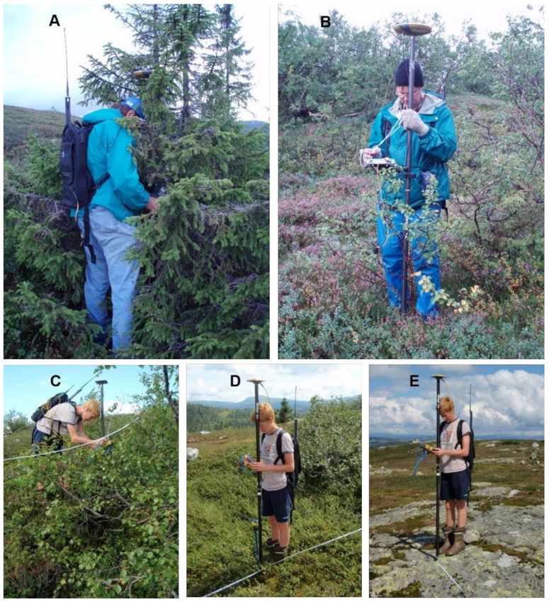
Figure 6. (A) Orthophoto of study area with manual delineation of the four sub-regions of Case
B; (B) Map with 5 m counter lines, the 12 tessellated cells of Case A (Cell 1–12), and boundaries
of the sub-regions for Case B (I–IV); (C) Predictions of vegetation height for the 1.5 m2 population
elements using ALS data; (D) Predictions of vegetation height for the 1.5 m2 population elements
using DAP data; (E) Estimated mean vegetation height using ALS data for tessellated cells of Case A;
(F) Estimated mean vegetation height using DAP data for tessellated cells of Case A; (G) Estimated
mean vegetation height using ALS for sub-regions of Case B; (H) Estimated mean vegetation height
using DAP for sub-regions of Case B. The vegetation height estimates for each domain in Figures
(E–H) are given by numbers.
Now, let U be the entire population of elements (the 79,242 elements of size 1.5 m2
tessellating the study area) where U = {1, . . . , k, . . . , N}. Furthermore, let ĥk denote the
predicted vegetation height according to the model in Equation (5) for element k. Thus, the
collection of spatially distributed predictions for the N elements constitutes the vegetationRemote Sens. 2021, 13, 2469 18 of 31
height maps mentioned above (Figure 6C,D). Mean vegetation height across the entire
study area can be estimated by the point estimator:
∑k∈U ĥk
ĥ = . (6)
N
This estimator can be used for smaller domains within the population as well.
2.7.3. Estimator of Mean Square Error
The term mean square error (MSE) rather than variance was used to characterize
the uncertainty of the model-dependent estimator in Equation (6) because the model-
dependent estimator of the population mean cannot be assured to be unbiased. For large
areas, model-dependent MSE estimators will, in general, depend mainly on the uncertainty
of the estimates of the model parameters (e.g., [55–57]). For small domains, an additional
source of uncertainty must often be accounted for, namely the residual variance. Ref. [58]
derived a model-dependent variance estimator that accounted for residual variance and
incorporated a spatial autocorrelation structure of the residuals. Ref. [52] demonstrated
with empirical data of timber volume from small forest stands and auxiliary data from DAP
that ignoring the residual variance component may induce bias in the mean square error
estimator. In the study on vegetation height change conducted in the current study area [12],
the analysis suggested that “ . . . most of the mean square error estimates (>95%) of the estimators
will be accounted for by quantifying the variance attributable to the model parameter uncertainty”.
Nevertheless, it cannot be assumed that the magnitude and spatial structure of the residual
variance of vegetation height predictions necessarily follow the same patterns as the
height change predictions. In the current study, we therefore addressed all the mentioned
components, i.e., (1) the variance due to uncertainty of the model parameters and the
residual (2) variance and (3) spatial covariance components. These three components
were treated as additive to obtain the total mean square error and will be described in
detail below.
Under the model-dependent inferential framework, the variance due to uncertainty of
the model parameters can be approximated either by using a closed-form formula based on
a first-order Taylor series approximation (see e.g., [57]), or by using Monte Carlo simulations
in the form of, for example, parametric bootstrap. Both approaches to estimation have been
adopted in forest- and vegetation-related studies in recent years (e.g., [50,59]). Ref. [60]
noted a few properties of parametric bootstrap that makes it attractive and demonstrated
the technique with ALS data. In the current study, we chose to adopt this technique,
as in Ref. [60]. In the following, it is assumed that the model parameter estimates of
the predictive model (β in the model in Equation (5)) follow asymptotically multivariate
normal distributions, i.e.:
β̂ ∼ N E[β], Σβ̂ , (7)
where the expected value of the vector of β̂ estimates is E[β] and Σβ̂ is the heteroscedasticity-
consistent estimates of the variance–covariance matrix of β̂.
By sampling from the multivariate distribution in
Equation (7), a large parametric
bootstrap sample of random vectors βPB ∼ N β̂, Σβ̂ was generated. The sample was
denoted SPB , where SPB = {1, . . . , l, . . . , M}. This sample can be used to produce new
predictions of h, according to Equation (5). Predictions of h were produced for all M random
vectors βPB and for all N population elements. Thus, we obtained unique predictions ĥPB,k,l
for k ∈ U and l ∈ SPB . A parametric bootstrap variance estimator for the point estimator in
Equation (6) is:
1 2
var ĥ
par
= ∑
M − 1 l ∈SPB
ĥ PB,l − ĥ PB , (8)
where:
1
ĥPB,l =
N ∑k∈U ĥPB,k,l (9)Remote Sens. 2021, 13, 2469 19 of 31
and:
1
M ∑l ∈SPB PB,l
ĥPB = ĥ . (10)
Analytical estimators for residual variance under heteroscedasticity have been adopted
in previous analysis of important parameters encountered in forest surveys, for example
timber volume [52]. In the current study, every geographical domain subject to estimation
had sample units (ground observations of vegetation height) that could be used to provide
estimates of residual variance. Thus, for a particular domain with a sample S with n sample
units, S = {1, . . . , k, . . . , n}, the residual variance for the point estimator for mean vegetation
height (Equation (6)) was formulated as [12]:
1 2
var ĥ
res
=
Nn ∑k∈S hk − ĥk . (11)
Residual covariance of substantial magnitude, as compared to the other sources of
uncertainty when estimating forest resource parameters for small areas, has been encoun-
tered for shorter distances in several studies (e.g., [52]), while at greater distances—and
consequently for larger areas—the residual covariance is often assumed or found to be
negligible in magnitude (e.g., [51]). However, as noted above, Ref. [12] found the residual
covariance to be negligible even for areas as small as 1.5 ha. Analytical ways of addressing
the residual covariance have been demonstrated by e.g., Ref. [52].
Quantifying the spatial autocorrelation of the residuals is essential in the analysis of
the residual covariance. Spatial correlation (ρ) is often estimated from the model prediction
residuals by constructing a correlogram. Assuming that a correlogram has been fitted and
that ρ can then be predicted to obtain predicted values of the correlation for all combinations
of the N population elements in U, the residual covariance for the point estimator of mean
vegetation height for a particular domain for which we had actual observations of the
residuals, can be estimated by [12]:
1 2
cov ĥ
res
=
nN 2 ∑k∈S hk − ĥk ∑k∈U ∑l∈U ρ̂kl , k 6= l , (12)
where ρ̂kl is the predicted value of the residual correlation between elements k and l in U
and the correlogram was fitted using the residuals hk − ĥk and hl − ĥl .
2.7.4. Calculations
The first step of the analysis was to construct the regression models for the ALS and
DAP data according to Equation (5) based on the 716 weighted sample observations. As
noted above, for the sake of comparison of estimates we also constructed simple models
according to Equation (5) without adopting the weighting scheme. These models are
nevertheless not documented in the current article.
Once the regression models were constructed, we proceeded with the estimation.
First, we estimated mean vegetation height across the entire study area, according to
Equation (6), by using model predictions from the height models (Equation (5)).
Two cases of special interest were identified. First (Case A), we tessellated the study
area into 1 ha cells that may serve as the primary mapping and monitoring units in,
for example, a tree line monitoring program (see Figure 6B). This size was chosen for
demonstration purposes, and this size can be changed to any size found meaningful for a
particular application. 1 ha resolution may be found useful for some applications, while,
for example, 100 m2 resolution may be found relevant for other applications. We could
even consider the primary resolution of 1.5 m2 , but some level of aggregation is in many
cases perhaps easier to comprehend and interpret. Another reason for choosing an area as
large as 1 ha was that a restricted number of cells (12) would ease the interpretation of any
potential differences in the properties of the estimates obtained from the two different 3D
remotely sensed datasets.You can also read