Towards improved turbulence estimation with Doppler wind lidar velocity-azimuth display (VAD) scans
←
→
Page content transcription
If your browser does not render page correctly, please read the page content below
Atmos. Meas. Tech., 13, 4141–4158, 2020
https://doi.org/10.5194/amt-13-4141-2020
© Author(s) 2020. This work is distributed under
the Creative Commons Attribution 4.0 License.

Towards improved turbulence estimation with Doppler
wind lidar velocity-azimuth display (VAD) scans
Norman Wildmann1 , Eileen Päschke2 , Anke Roiger1 , and Christian Mallaun3
1 Deutsches Zentrum für Luft- und Raumfahrt e.V., Institut für Physik der Atmosphäre, Oberpfaffenhofen, Germany
2 DWD,  Meteorologisches Observatorium Lindenberg – Richard-Aßmann-Observatorium, Lindenberg, Germany
3 Deutsches Zentrum für Luft- und Raumfahrt e.V., Flugexperimente, Oberpfaffenhofen, Germany

Correspondence: Norman Wildmann (norman.wildmann@dlr.de)

Received: 12 January 2020 – Discussion started: 5 February 2020
Revised: 1 July 2020 – Accepted: 3 July 2020 – Published: 4 August 2020

Abstract. The retrieval of turbulence parameters with pro-       pation rate retrieval from 75◦ VAD scans at the lowest mea-
filing Doppler wind lidars (DWLs) is of high interest for        surement heights. Successive scans at 35.3 and 75◦ from the
boundary layer meteorology and its applications. DWLs pro-       CoMet campaign are shown to provide TKE dissipation rates
vide wind measurements above the level of meteorologi-           with a good correlation of R > 0.8 if all corrections are ap-
cal masts while being easier and less expensive to deploy.       plied. The validation against the research aircraft encourages
Velocity-azimuth display (VAD) scans can be used to retrieve     more targeted validation experiments to better understand
the turbulence kinetic energy (TKE) dissipation rate through     and quantify the underestimation of lidar measurements in
a fit of measured azimuth structure functions to a theoreti-     low-turbulence regimes and altitudes above tower heights.
cal model. At the elevation angle of 35.3◦ it is also possible
to derive TKE. Modifications to existing retrieval methods
are introduced in this study to reduce errors due to advec-
tion and enable retrievals with a low number of scans. Data      1   Introduction
from two experiments are utilized for validation: first, mea-
surements at the Meteorological Observatory Lindenberg–          The observation of turbulence in the atmosphere, in partic-
Richard-Aßmann Observatory (MOL-RAO) are used for the            ular the atmospheric boundary layer (ABL), is of great im-
validation of the DWL retrieval with sonic anemometers on        portance for basic research in boundary layer meteorology
a meteorological mast. Second, distributed measurements of       and in applied fields such as aviation, wind energy (van Kuik
three DWLs during the CoMet campaign with two different          et al., 2016; Veers et al., 2019), and pollution dispersion
elevation angles are analyzed. For the first time, the ground-   (Holtslag et al., 1986).
based DWL VAD retrievals of TKE and its dissipation rate            A wide range of instruments are used to measure turbu-
are compared to in situ measurements of a research aircraft      lence: sonic anemometers are currently the most popular in
(here: DLR Cessna Grand Caravan 208B), which allows for          situ instrument that can be installed on meteorological masts
measurements of turbulence above the altitudes that are in       and provide continuous data on three-dimensional flow and
range for sonic anemometers.                                     its turbulent fluctuations (Liu et al., 2001; Beyrich et al.,
    From the validation against the sonic anemometers we         2006). For in situ measurements above the height of tow-
confirm that lidar measurements can be significantly im-         ers, airborne systems are applied such as manned aircraft
proved by the introduction of the volume-averaging effect        (Bange et al., 2002; Mallaun et al., 2015), remotely piloted
into the retrieval. We introduce a correction for advection in   aircraft systems (RPAS; van den Kroonenberg et al., 2011;
the retrieval that only shows minor reductions in the TKE        Wildmann et al., 2015), or tethered lifting systems (TLSs;
error for 35.3◦ VAD scans. A significant bias reduction can      Frehlich et al., 2003), which can be equipped with turbulence
be achieved with this advection correction for the TKE dissi-    probes such as multi-hole probes or hot-wire anemometers.
                                                                 A different category of instruments includes remote sensing

Published by Copernicus Publications on behalf of the European Geosciences Union.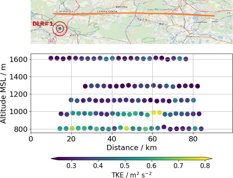
4142                   N. Wildmann et al.: Towards improved turbulence estimation with Doppler wind lidar VAD scans

instruments such as radar, sodar, and lidar, which can mea-         the cone diameter of the VAD scan is small. With this study,
sure wind speeds and allow for the retrieval of turbulence          we propose a method to reduce this error. We also apply the
based on assumptions of the state of the atmosphere and the         turbulence retrieval to VAD scans with a 75◦ elevation an-
structure of turbulence. In this study, we focus on ground-         gle, which still allows for the retrieval of the TKE dissipation
based Doppler wind lidars (DWLs), which have become in-             rate. In this case the advection correction is particularly im-
creasingly popular in boundary layer research because of            portant. The experiments that were carried out are explained
their ease of installation, invisible and eye-safe lasers, re-      in Sect. 2. The methods and the new developments are ex-
liability, and high availability, which is only restricted by       plained in Sect. 3. A focus of this study is on the validation
clouds, fog, and rain or very low aerosol content in the at-        of the lidar measurements with sonic anemometers and air-
mosphere.                                                           borne in situ measurements. The results of the validation are
   A variety of methods already exist to retrieve turbulence        presented in Sect. 4. Conclusions and an outlook are given in
from DWL measurements. They can be categorized accord-              Sect. 5.
ing to the respective scanning strategy applied: the simplest
scanning pattern is a constant vertical stare to zenith, which
allows researchers to obtain variances of vertical velocity         2     Experiment description
and estimates of the turbulence kinetic energy (TKE) dissi-
                                                                    In this study, data from two different experiments are ana-
pation rate (O’Connor et al., 2010; Bodini et al., 2018). More
                                                                    lyzed. Both of the experiments and the instrumentation are
complex are conical scans (velocity-azimuth display, VAD)
                                                                    introduced in this section.
with continuous measurements along the cone (Banakh et al.,
1999; Smalikho, 2003; Krishnamurthy et al., 2011; Smalikho          2.1    The MOL-RAO Falkenberg field site
and Banakh, 2017). These scans include information on the
horizontal wind component as well. A simplification of VAD          The Meteorological Observatory Lindenberg–Richard-
scans are Doppler-beam-swinging (DBS) methods that re-              Aßmann Observatory (MOL-RAO) is part of Deutscher
duce the number of measurements taken along the cone to             Wetterdienst (DWD), the national meteorological service
a minimum of four to five beams and thus increase the up-           of Germany. The observatory is situated in the east of
date rate for single wind profile estimations (Kumer et al.,        Germany, approximately 65 km to the southeast of the center
2016). Both VAD and DBS are popular scanning strategies             of Berlin. MOL-RAO runs a comprehensive operational
that are applied in commercial instruments. Kelberlau and           measurement program to characterize the physical structure
Mann (2019, 2020) introduced new methods to obtain bet-             and processes in the atmospheric column above Lindenberg.
ter turbulence spectra from conically scanning lidars with          Measurements of ABL processes form an essential part
corrections for the scanner movement. Significantly differ-         of it; they are carried out at the boundary layer field site
ent scanning strategies are vertical (or horizontal) scans that     (in German: Grenzschichtmessfeld, GM) in Falkenberg,
can also provide vertical profiles of turbulence (Smalikho          about 5 km to the south of the main observatory site. The
et al., 2005) but even allow for the derivation of the two-         GM Falkenberg is situated in a rural landscape dominated
dimensional fields of the TKE dissipation rate (Wildmann            by forest, grassland, and agricultural fields (see Fig. 1). A
et al., 2019). Multi-Doppler measurements require more than         central measurement facility at the Falkenberg site is a 99 m
one lidar with intersecting beams but do not need assump-           tower, equipped with booms to carry sensors every 10 m.
tions on homogeneity to measure turbulence at the points of            Since 2014, MOL-RAO has been using a DWL “Stream
the intersection directly (Fuertes et al., 2014; Pauscher et al.,   Line” (Halo Photonics Ltd.) for boundary layer measure-
2016; Wildmann et al., 2018). For operational or continu-           ments. From that time the device has been extensively tested
ous monitoring of the vertical profiles of turbulence in the        with respect to its operational use for wind and turbulence
ABL, VAD or DBS scans are most suitable. At an eleva-               measurements. This included, for instance, tests of the tech-
tion angle of 35.3◦ , a VAD scan allows for the retrieval of        nical robustness and data availability under all weather con-
TKE and its dissipation rate, integral length scale, and mo-        ditions, but also tests of different scanning strategies and re-
mentum fluxes according to a method that was first devel-           trieval methods for the 3D wind vector and for the TKE. The
oped for radar by Kropfli (1986) and adapted for lidar later        position of the DWL during a measurement period from 2
by Eberhard et al. (1989) using the variance of radial veloci-      through 30 April 2019 was at the western edge of the field
ties along the scanning cone. Further improvements of this          site at about 500 m of distance from the 99 m tower. It should
method have been implemented by Smalikho and Banakh                 be noted that there is a small patch of forest about 300 m to
(2017) and Stephan et al. (2018), which also account for lidar      the W-NW of the lidar site. During this period the system
volume-averaging effects. We introduce modifications to the         continuously performed VAD scans with an elevation angle
estimation of structure function and variances in order to be       of 35.3◦ , which will be analyzed for turbulence retrievals in
able to retrieve turbulence parameters from a smaller number        this study.
of VAD scans. For conditions with significant advection, the
method can cause errors, especially at low altitudes at which

Atmos. Meas. Tech., 13, 4141–4158, 2020                                              https://doi.org/10.5194/amt-13-4141-2020
N. Wildmann et al.: Towards improved turbulence estimation with Doppler wind lidar VAD scans                              4143

                                                                 tinuously measuring. The locations of the three lidars were
                                                                 planned to cover the whole region of interest and were finally
                                                                 chosen based on logistical constraints.
                                                                    The lidars were operating in VAD modes with two differ-
                                                                 ent elevation angles. Since the focus for the CoMet campaign
                                                                 was on continuous wind profiling and a good height coverage
                                                                 was desired, the lidars were programmed to perform VADs
                                                                 with an elevation angle of 75◦ (see Table 1, VAD75) for a
                                                                 longer period, i.e., 24 scans (≈ 29 min), followed by only six
                                                                 scans (≈ 7 min) at a 35.3◦ elevation (VAD35) for turbulence
                                                                 retrievals.
                                                                    As shown in Fig. 2, the three lidars were separated by sev-
                                                                 eral tens of kilometers and were located in different terrain
                                                                 types. While DWL no. 1 was in a mixed rural and urban
                                                                 area, DWL no. 2 was in a mostly forested environment, and
Figure 1. Sketch of the measurement site at MOL-RAO, GM          DWL no. 3 was in close vicinity to the lake Goczałkowicki.
Falkenberg. Map data © OpenStreetMap contributors 2019. Dis-     The main wind direction during the campaign was from the
tributed under a Creative Commons BY-SA License.                 east, with particularly strong winds during nighttime low-
                                                                 level jet (LLJ) events. In this study we analyze statistics of
                                                                 the whole campaign, as well as a case study on 5 June 2017,
   Continuous turbulence measurements (20 Hz sampling            on which D-FDLR was performing long straight and level
frequency) using a sonic anemometer of type USA-1                legs between 800 and 1600 m as indicated in the flight path
(METEK GmbH) are performed at the 50 and 90 m levels on          in Fig. 2. Since the D-FDLR was focusing on GHG measure-
the tower and have been used for validation purposes. The        ments at the hotspots of the Upper Silesian Coal Basin, there
instruments are mounted at the tip of the booms pointing to-     are no more straight and level flight paths that allow for tur-
wards south.                                                     bulence retrieval. For this day, however, the research aircraft
                                                                 provides a unique possibility to validate lidar measurements
2.2   The CoMet (CO2 and Methane) mission 2018                   with in situ measurements at higher altitudes that cannot be
                                                                 reached with sonic anemometers. The flow probe and iner-
Within the scope of the CO2 and Methane (CoMet) mission          tial measurement unit on the D-FDLR are well-established
that was conducted in spring 2018, three Doppler wind li-        instruments that allow for reliable measurements of the 3D
dars of type Leosphere Windcube 200S (details see Table 1)       wind vector and turbulence (Mallaun et al., 2015).
were installed in Upper Silesia (Poland) with the purpose of
providing spatially distributed wind and turbulence measure-
ments in the ABL. CoMet aims at a better understanding of        3     Methods
the budgets of the two most important anthropogenic green-
                                                                 3.1    Sonic anemometer turbulence measurements
house gases (GHGs), CO2 and CH4 . For this purpose, the
research aircraft HALO (high altitude and long range) was        From the sonic anemometers on the meteorological
taking remote sensing and in situ measurements over large        mast, TKE and the TKE dissipation rate are calculated.
parts of the European continent. A dedicated area of high in-    TKE is calculated
terest was the region of Upper Silesia, where large amounts                           from the sum of variances ETKE =
                                                                 0.5 σu2 + σv2 + σw2 . The TKE dissipation rate ε is estimated
of methane are known to be released due to the intensive coal    through a fit of the theoretical longitudinal Kolmogorov
extraction activities in the coal basin. During the CoMet cam-   structure function in the range τ1 = 0.1 s to τ2 = 2 s to the
paign, the DLR Cessna Grand Caravan 208B (D-FDLR) air-           measured second-order structure function of horizontal ve-
craft was equipped with in situ instruments to measure green-    locity. Muñoz-Esparza et al. (2018) showed that the structure
house gases and thermodynamic variables.                         function method is more robust than estimates from spectra.
   The DWL measurements are particularly helpful to sup-         For this study, in order to have the best possible compari-
port the CoMet measurements by providing wind informa-           son to the lidar measurements the values for ε are calculated
tion that is essential to derive emission flux estimates from    for 30 min intervals. The geometry of the sonic anemome-
passive remote sensing (Luther et al., 2019) or in situ mea-     ter setup disturbs the measurements for wind directions from
surements of mass concentrations (Fiehn et al., 2020). The       330 to 50◦ (see also Appendix D). Data for these wind direc-
DWL wind information can also be used to validate modeled        tions are removed from the analysis.
wind from the transport models for greenhouse gases. The
lidars were remotely operated during the whole CoMet cam-
paign period from 16 May to 17 June 2017 and were con-

https://doi.org/10.5194/amt-13-4141-2020                                          Atmos. Meas. Tech., 13, 4141–4158, 2020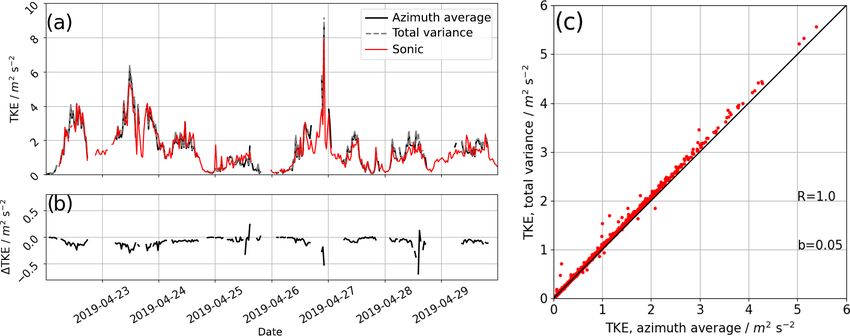
4144                        N. Wildmann et al.: Towards improved turbulence estimation with Doppler wind lidar VAD scans

Table 1. Main technical specifications of the Doppler wind lidars.

                                                              Windcube 200S,       Windcube 200S,      Stream Line
                                                              VAD75                VAD35
                               Wavelength λ                   1.54 µm              1.54 µm             1.5 µm
                               Pulse length τp                200 ns               200 ns              180 ns
                               Time window Tw                 288 ns               144 ns              240 ns
                               Bandwidth                      26.7 m s−1           26.7 m s−1          19.4 m s−1
                               Elevation angle ϕ              75◦                  35.3◦               35.3◦
                               Angular speed                  5◦ s−1               5◦ s−1              5◦ s−1
                               Pulse repetition frequency     20 kHz               20 kHz              15 kHz
                               Accumulation time              200 ms               200 ms              133 ms
                               CNR filter                     −20.0 dB             −20.0 dB            −15.0 dB

                                                                           ETKE is derived:

                                                                                 3
                                                                           ETKE = σ 2r |ϕ=35.3◦ .                                      (3)
                                                                                 2

                                                                           In this equation, σ 2r is the mean of the variance of radial ve-
                                                                           locities over all azimuth angles. In the following, we will re-
                                                                           fer to this method as E89 retrieval.
                                                                              In order to retrieve estimations of the TKE dissipation rate
                                                                           ε from VAD scans, a similar approach to the method for sonic
                                                                           anemometers can be followed. A fit of the equation

                                                                           Dr (ψ) = (4/3)CK (εψR 0 )2/3                                (4)

                                                                           to the azimuth structure function yields an estimate for ε ac-
                                                                           cording to Smalikho and Banakh (2017). In Eq. (4) Dr is
Figure 2. Sketch of the measurement site in Upper Silesia. Red cir-        the transverse structure function of radial velocities, CK the
cles show the extent of the VAD scan at 35.3◦ for 100 and 2000 m at        Kolmogorov constant, ψ the azimuth angle increment, and
the respective lidar location. The orange line marks the flight path of
                                                                           R 0 = R cos ϕ. We will refer to this method as S17A in the
D-FDLR on 5 June 2017. The different shades of orange are used to
                                                                           following.
indicate a subdivision of the flight leg in shorter sub-legs. Map data
© OpenStreetMap contributors 2019. Distributed under a Creative               Scanning with Doppler lidar in a classical VAD with con-
Commons BY-SA License.                                                     tinuous motion of the azimuth motor involves a volume aver-
                                                                           aging of radial velocities in the longitudinal (along the laser
                                                                           beam) and transverse (orthogonal to the beam) direction. The
3.2     VAD turbulence measurements                                        E89 and S17A methods do not consider this effect and will
                                                                           thus yield a systematic underestimation of TKE and ε. Sma-
Methods to retrieve turbulence parameters from VAD scans                   likho and Banakh (2013) proposed a theory that considers the
are well-known and a variety of different methods exist. The               volume averaging and allows for the retrieval of ε from con-
method we refine in this study is based on the theory that                 ical scans, independent of the elevation angle. In Smalikho
was originally described by Eberhard et al. (1989) for lidar               and Banakh (2017), this method has been combined with the
measurements. The variance of radial velocities σr2 depends                E89 method to yield TKE, ε, and the momentum fluxes. It
on the range gate distance R, the azimuth angle θ , and the                is based on the decomposition of radial velocity variance σr2
elevation angle ϕ. It is calculated from the measured radial               into its subcomponents, i.e.,
velocities Vr :
                                                                           σL2 = σa2 + σe2 ,                                           (5)
vr (R, θ, ϕ, t) = Vr (R, θ, ϕ, t) − hVr (R, θ, ϕ)i,                (1)     σa2   = σr2 − σt2 ,                                         (6)
σr2                     2
      = hvr (R, θ, ϕ, t) i.                                        (2)     σr2   = σL2 + σt2 − σe2 ,                                   (7)

  From a partial Fourier decomposition (see Appendix A)                    where σL2 is the lidar-measured variance, σa2 is the lidar-
and for the special case of ϕ = 35.3◦ , a simple equation for              measured variance without instrumental error σe2 , and σt2 is

Atmos. Meas. Tech., 13, 4141–4158, 2020                                                         https://doi.org/10.5194/amt-13-4141-2020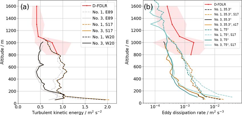
N. Wildmann et al.: Towards improved turbulence estimation with Doppler wind lidar VAD scans                                     4145

the turbulent broadening of the lidar measurement. In Sma-
likho and Banakh (2017), all of these variances and structure
functions are calculated for single azimuth angles and then
averaged. We describe in Sect. 3.2.1 why we use the total
variances and structure functions of all radial velocities.
   The measured azimuth structure function Da (ψl ) is a func-
tion of the separation angle ψl , where l is the index of the
discrete separation angle of the scan. It can be decomposed
into the lidar-measured structure function DL (ψl ) and the in-
strumental error σe2 :

DL (ψl ) = h[vr (θ ) − vr (θ + ψl )]2 i,                   (8)
Da (ψl ) = DL (ψl ) − 2σe2 .                               (9)

  Combining Eq. (7) with Eq. (9) yields
                 1          1
σr2 = σL2 + σt2 − DL (ψl ) + Da (ψl ).                    (10)
                 2          2
                                                                  Figure 3. Example of the structure functions of sonic anemometer
   It shows that since the instrumental error σe2 is assumed
                                                                  (blue) and lidar (grey) at 90 m of height on 4 April 2019, 12:00–
to be a constant offset of azimuth structure function Da (ψl )    12:30 UTC. The dashed black line shows the measured lidar struc-
and the lidar measurement DL (ψl ), l can be chosen arbitrar-     ture function DL , and the solid black line Da is corrected for the
ily here. It is set to l = 1 because potential random errors      systematic error σe (see Eq. 9). The grey dashed line gives the model
like nonstationary flow will be smaller for small separation      structure function A, and the dotted lines indicate the reconstructed
angles. Using Eqs. (3) and (21) (see Sect. 3.2.1), TKE can        inertial subrange for the calculated values of ε. The parts with bold
be redefined as a function of the measured line-of-sight vari-    lines are those ranges that are used for the structure function fits.
ances σL2 , the measured lidar azimuth structure function of
radial velocities DL (ψ1 ), and a residual term G, which in-
cludes the two unknowns, σt2 and Da (ψ1 ):                          Using Eqs. (14) and (9), ε can be retrieved from Da (ψl ) −
                                                                Da (ψ1 ):
         3 2 DL (ψ1 )
ETKE =        σ −           +G ,                         (11)           DL (ψl ) − DL (ψ1 ) 3/2

         2 L           2                                          ε=                            .                         (16)
            1                                                           A(l1y) − A(1y)
G = σt2 + Da (ψ1 ).                                      (12)
            2                                                     This equation does not depend on the elevation angle so that
   In Banakh and Smalikho (2013), a relationship between          the method allows for the retrieval of ε from VAD scans
the two unknowns and the TKE dissipation rate is theo-            with elevation angles different from 35.3◦ as well. Figure 3
retically derived from the two-dimensional Kolmogorov–            gives an example of the different structure functions that are
Obukhov spectrum as                                               calculated in this method (i.e., DL , Da , and A) and also
                                                                  gives a comparison to the structure function Ds as calcu-
σt = ε 2/3 F (1y),                                        (13)    lated from sonic anemometer measurements. Smalikho and
Da (ψl ) = ε 2/3 A(l1y),                                  (14)    Banakh (2017) found a separation angle of l1θ = 9◦ to be
                                                                  an appropriate value for ABL measurements. In this study,
where F (1y) and A(l1y) are model functions that include          all VAD scans are performed with a resolution of 1θ = 1◦
the lidar filter functions (see Appendix B). The lidar filter     so that l = 9. In Fig. 3 the range that is thus used for the
functions in the longitudinal direction depend on the pulse       structure function fit is indicated by the bold black line.
width of the laser beam 1p and the time window Tw of the             The retrieval method for ε using Eq. (16) and TKE using
data acquisition. The transverse filter function is defined by    Eq. (11) will be referred to as S17 in the following.
1y = R1θ cos ϕ, which is the distance the lidar beam moves
along the cone during one accumulation period. The param-         3.2.1   Modifications for a small number of scans
eters for the lidars in this study are provided in Table 1 and
                                                                  The VAD at ϕ = 35.3◦ during the CoMet campaign was not
are calculated from information given by the manufacturer
                                                                  run continuously, but only six individual scans were per-
for the specific lidar type. Hence, G depends on the turbu-
                                                                  formed successively before switching back to the VAD at
lence dissipation rate ε:
                                                                  ϕ = 75◦ as described in Sect. 2.2. This means that only six

                       A(1y)                                      data points are available to calculate the variance and mean of
G = ε 2/3 F (1y) +               .                        (15)    the radial velocities at each azimuth angle, which cannot be
                          2

https://doi.org/10.5194/amt-13-4141-2020                                             Atmos. Meas. Tech., 13, 4141–4158, 2020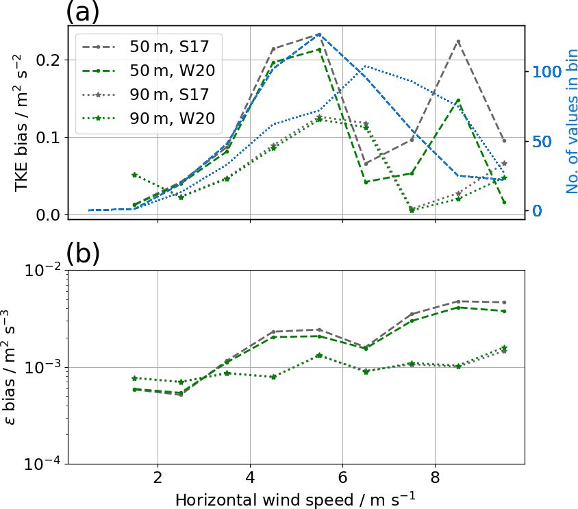
4146                       N. Wildmann et al.: Towards improved turbulence estimation with Doppler wind lidar VAD scans

considered a solid statistic. We introduce two modifications        3.2.2     Filtering of bad estimates
of data processing to overcome this problem that are based on
the assumptions of stationary and homogeneous turbulence.           Improvements of turbulence estimates in low signal con-
                                                                    ditions can be achieved by filtering bad estimates as de-
Practical implementation of the ensemble average                    scribed in Stephan et al. (2018). This approach is not based
                                                                    on the calculation of the azimuth structure function from
In Eq. (2), hVr (R, θ, ϕ)i can be calculated as the arithmetic      measured radial velocities but uses probability density func-
mean of radial velocities at specific azimuth angles:               tions (PDFs) and their corresponding standard deviations.
                                                                    The model PDF is defined as a Gaussian function with a filter
                       N
                    1 X                                             term P :
hVr (R, θ, ϕ)i =          Vr (R, θn , ϕ),                   (17)
                    N n=0
                                                                               1−P           1  x 2     P
                                                                    pM (x) = √       exp −              +    ,               (23)
where N is the number of scans. Instead of this approach,                       2π σ         2 σ          Bv
we suggest using the reconstructed radial velocity from the
retrieved wind field over all individual scans as the expected      where P is the probability of bad estimates of x, σ is the
value in the variance calculation. For the retrieval of the three   standard deviation of the PDF, and Bv is the velocity band-
wind components (û, v̂, ŵ), filtered sine-wave fitting (FSWF)     width of the lidar. Equation (23) is fit to the observed dis-
is applied (Smalikho, 2003). The reconstructed radial veloc-        tributions of vr (R, θ ), 1vr (R, θ + 1θ ), and 1vr (R, θ + l1θ )
ities V̂ are then used as the expected value in the variance        by adjusting the corresponding values σ1 , σ2 , and σ3 and the
calculation:                                                        probability of bad estimates P1 , P2 , and P3 . The values of σi
                                                                    are used as the first guess of the standard deviation of the dis-
V̂ = ŵ(R) sin ϕ + v̂(R) cos ϕ cos θ + û(R) cos ϕ sin θ,   (18)    tributions. However, since the PDFs cannot be assumed to be
                                                                    Gaussian in atmospheric turbulence, the standard deviations
hVr (R, θ, ϕ)i = V̂ (R, θ, ϕ).                              (19)    are finally calculated as the integral over the measured PDFs
                                                                    in the range ±3.5σ according to Stephan et al. (2018).
With this approach, all measurement points in the VAD
                                                                       Replacing σL2 with σ12 , DL (ψ1 ) with σ22 , and DL (ψl ) with
with the same elevation angle are used to obtain the ex-              2
                                                                    σ3 in Eqs. (11) and (16) yields
pected value hVr i, and thus a better statistical significance is
achieved. This method has also been proposed in Smalikho                     "            #
and Banakh (2017) as a practical implementation of Eq. (2).                3    2  σ22
                                                                    ETKE =     σ −     +G                                       (24)
                                                                           2 1      2
Averaging of variances
                                                                    and
In Smalikho and Banakh (2017), the variances of the lidar
                                                                                             #3/2
measurements are defined as the average of variances at in-
                                                                          "
                                                                           σ32 − σ22
dividual azimuth angles:                                            ε=                              .                           (25)
                                                                       A(l1y) − A(1y)
            M
         1 X
σ 2r =        σ 2 (θm ).                                    (20)       As suggested in Stephan et al. (2018), Eqs. (24) and (25)
         M m=0 r                                                    are only used if P > 0. We also introduced a quality control
                                                                    to discard any measurements with P > 0.5 for best results.
   The variances σr2 (θm ) are the variances of a subsample of      In practice, this method will thus only be applied in some
the radial velocities of the VAD (i.e., those at a specific az-     conditions when the signal is weak and can extend the range
imuth angle θm ). We use a simple relation between the vari-        of vertical profiles to some degree.
ances of subsamples and the total variance of a dataset (see
Appendix C). Applying this to the radial velocity variances         3.2.3     Correction for advection
yields
                                                                    The azimuth structure function and the volume-average filter
             g
      k−1 X 2              k(g − 1)                                 are distorted by advection through a modification of 1y. The
σr2 =           σr (θm ) +          vr,                     (21)
      n − 1 m=1             k−1                                     effect is illustrated in Fig. 4. It shows that the distance be-
                                                                    tween measurement points in a flow-fixed coordinate system
where k is the number of samples at each azimuthal angle,           is unequally spaced and on average larger than in the earth-
g is the number of subsamples, and n is the number of total         fixed coordinate system. We propose a simplified correction.
samples in the dataset (n = gk). Since the mean of the radial       When advection is not considered, the spacing between sam-
velocity fluctuations is zero by definition, Eq. (21) becomes       ples is given by

σr2 ≈ σ 2r (θm ).                                           (22)    1y = 1θ R cos ϕ.                                            (26)

Atmos. Meas. Tech., 13, 4141–4158, 2020                                               https://doi.org/10.5194/amt-13-4141-2020
N. Wildmann et al.: Towards improved turbulence estimation with Doppler wind lidar VAD scans 4147
Table 2. Overview of turbulence retrieval methods and the applied
filters and methods.
E89 S17A S17 W20
TKE yes yes yes yes
ε no yes yes yes
Lidar volume-averaging effect no no yes yes
CNR filter yes yes yes no
Filter of bad estimates no no no yes
Integral length scale filter yes yes yes yes
Advection filter no no yes no
Advection correction no no no yes
Variance modifications yes yes yes yes
Figure 4. Sketch of the measurement points of a VAD scan in an
the data are filtered according to the criteria given in Sma-
earth-fixed versus a flow-fixed coordinate system. likho and Banakh (2017):
l1y
Lv , (31)
An estimate of the mean spacing can be obtained from Lv > max {1z, 1y} , (32)
0
1 XN q R ωs
|hV i|. (33)
1y ≈ dxi2 + dyi2 , (27)
N i=0 For the purpose of evaluating the methods in a broad range,
we set mild criteria for Eqs. (31) and (33) using
where dxi = xi+1 − xi . We propose a simplified correction in
which l1y < 2Lv (34)
N q
1 X 2 + dy 2 ,
1yc ≈ dxc,i c,i (28) and
N i=0
R 0 ωs > 2|hV i|. (35)
where
dxc,i = dxi + cos 9U 1t, (29) Equations (31) and (32) are criteria that require the integral
length scale Lv to be larger than the sensing volume of the
dyc,i = dyi + sin 9U 1t. (30) lidar in the transversal (1y) and longitudinal (1z) direction.
Unfortunately, there is no independent measurement of Lv
Here, R is the range gate distance, ϕ is the elevation an- at all heights of the VAD scan so that it is derived from the
3/2
gle, xi and yi are the measurement point locations, 9 is wind lidar measurement itself as Lv = 0.3796 Eε (Smalikho and
direction, U is wind speed, and 1t is the accumulation time Banakh, 2017).
of the lidar. The terms cos 9U 1t and sin 9U 1t describe the The filter criteria in Eq. (33) provide a filter for conditions
effect of advection on the measurement location in the x and with significant advection, which distorts the measured struc-
y direction, respectively. Using the corrected measurement ture functions and is only applied if the method described in
location displacements dxc,i and dxc,i , we can calculate a Sect. 3.2.3 is not used.
corrected mean transverse sensing volume 1yc . This method Except for the retrieval method W20, which uses the fil-
does not account for the unequal spacing but corrects the av- tering of bad estimates, we set fixed CNR filter thresholds
erage separation of data points, which is particularly impor- adapted to the lidar type. Since the turbulence retrievals are
tant for the statistical evaluation of turbulence. very sensitive to bad estimates, we set the CNR thresholds to
The effects of advection on the turbulence estimation are conservative values that are given in Table 1.
largest in the lowest levels of the VAD scans because 1y is An overview of all retrieval methods and their characteris-
small compared to U 1t in this case. The retrieval method tics and filters that are applied is given in Table 2.
including filtering for bad estimates and the advection cor-
rection is referred to as W20 in the following. 3.3 Turbulence estimation from airborne data
3.2.4 Quality control filters The estimation of turbulence parameters from the wind mea-
surement system on the DLR Cessna Grand Caravan 208B
In order to fulfill the assumptions that are made with regards (Mallaun et al., 2015) is done very similarly to the in situ
to the turbulence model and the turbulence retrieval method, estimations from the sonic anemometer. TKE is calculated
https://doi.org/10.5194/amt-13-4141-2020 Atmos. Meas. Tech., 13, 4141–4158, 20204148 N. Wildmann et al.: Towards improved turbulence estimation with Doppler wind lidar VAD scans
from the sum of variances as described in Sect. 3.1. The dis- locities at individual azimuth angles. It is small enough to be
sipation rate is also calculated from the second-order struc- neglected for further analysis.
ture function but with different bounds for the time lag. For
the flight data we use τ1 = 0.2 s and τ2 = 2 s, corresponding 4.1.2 Comparison of lidar retrievals
to approximately 13–130 m lag at 65 m s−1 mean airspeed.
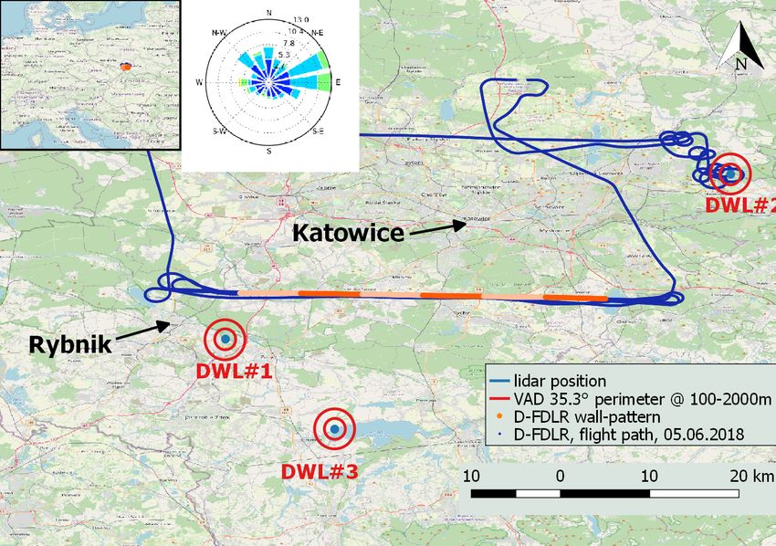
To evaluate the heterogeneity of turbulence due to chang-
The MOL-RAO dataset allows us to compare the retrievals
ing land use along the flight legs of more than 50 km length,
without consideration of lidar volume averaging (E89 and
we divided the legs into sub-legs of 6.5 km (i.e., 100 s averag-
S17A) to the S17 retrieval and its modified version W20 in-
ing time) and calculated turbulence for each leg individually.
troduced in this study. For this purpose, the individual re-
The location of the legs and the sub-legs is shown in Fig. 2.
trieval results are compared to the sonic anemometer esti-
mates of TKE and its dissipation rate ε. Figure 6 shows the
4 Validation scatterplots for TKE at the two measurement levels. For each
method, the coefficient of determination Rc2 of the linear re-
4.1 Comparison to sonic anemometer gression between the sonic measurement and lidar retrieval
is given, as is a bias that is calculated as b = (y − x) for
The best possible validation of the methods introduced in
TKE and blog = log10 y − log10 x for ε. We find that with
Sect. 3 can be performed with the lidar in close proximity the E89 method, TKE is systematically underestimated, as
to the meteorological mast such as at the measurement site expected. In contrast to that, the S17 method yields slightly
at MOL-RAO. The sonic anemometers at 50 and 90 m on the overestimated TKE values if no advection filter is applied
mast almost coincide with the measurement levels of the lidar (light red dots) but good agreement with the sonic anemome-
at 52 and 93.6 m, respectively. Since the VAD retrieval with ter in the absence of advection (red dots). The overestima-
an elevation angle of 35.3◦ yields TKE and its dissipation tion of TKE is larger for the lower level at 50 m compared
rate, both turbulence parameters can be compared to values to the 90 m level, which we attribute to the smaller averag-
obtained from the sonic anemometers. In this section we will ing volume 1y. Our refined version of the retrieval including
evaluate the methods described in Sect. 3.2, in particular the the advection correction improves the results slightly, espe-
validity of the assumptions made in Sect. 3.2.1 and the effi- cially for the high-turbulence cases (corresponding to high
ciency of the advection correction described in Sect. 3.2.3. wind speeds) at the 50 m level, as the scatterplots show. Fig-
ure 7 gives the scatterplot comparison of ε retrieval from
4.1.1 Validation of modified variance S17A, S17, and W20 with the sonic anemometer. E89 does
not provide an estimate for ε. Even more clearly than for
In Sect. 3.2.1 we introduced two modifications to the calcu-
TKE, the underestimation of the method without consid-
lation of the averaged lidar radial velocity variances. These
eration of lidar volume averaging (S17A) is found. Also,
changes are especially necessary if a low number of VAD
a now positive bias of b = 0.09 m2 s−2 for lidar estimates
scans is used for turbulence retrieval. In the MOL-RAO ex-
with the S17 method at the 50 m level is reduced with the
periment, VAD scans are run continuously with ϕ = 35.3◦ so
advection correction to b = 0.06 m2 s−2 . It is evident from
that the modifications can be tested against the original ver-
the ε estimates that all lidar retrievals underestimate turbu-
sion of the retrieval method. The sonic anemometer at 90 m
lence significantly compared to the sonic anemometer in the
on the meteorological mast serves as an independent vali-
low-turbulence regimes, in particular for values smaller than
dation measurement. Figure 5a shows a time series of the
2 × 10⁻³ m2 s−3 , which is why these values have been ex-
two methods and the sonic anemometer in a time period in
cluded for the estimation of biases (grey dots).
which all systems were providing good data almost without
interruption (22–29 April 2019). The lidar retrieval with both
variance methods follows the sonic anemometer TKE esti- 4.1.3 Evaluation of advection error
mation very well through the diurnal cycles, with some oc-
casional overestimation that will be discussed in Sect. 4.1.2. To evaluate the error that is caused by advection in the S17
Figure 5b gives the difference (1TKE) between the azimuth retrieval, all data that were collected at MOL-RAO were
average and total average to show that it is typically below binned into wind speeds with a bin width of 1 m s−1 . The
0.5 m2 s−2 except for some periods with strong gradients in mean absolute error between the lidar retrievals and the sonic
TKE. Figure 5c shows the scatterplot that directly compares anemometers at the respective level is calculated and shown
the S17 retrieval calculated with azimuth-averaged variances in Fig. 8 for TKE and ε. Although the averaged errors of TKE
to the S17 retrieval using total variances. There is a higher are small in general, it shows that the W20 method does re-
estimation of TKE in the total variance method, which in- duce the error in comparison to the S17 method at the 50 m
creases with TKE. We cannot fully explain this effect at this level. The error for ε at the 50 m level increases with wind
point, but it might be due to the small-scale turbulence that speed but less for the W20 method. Hardly any improvement
cannot be resolved with the 72 s sampling rate of radial ve- is found for the already small errors of TKE and ε at 90 m.
Atmos. Meas. Tech., 13, 4141–4158, 2020 https://doi.org/10.5194/amt-13-4141-2020N. Wildmann et al.: Towards improved turbulence estimation with Doppler wind lidar VAD scans 4149 Figure 5. Time series of TKE from lidar retrievals compared to a sonic anemometer at 90 m above ground level (a), the difference between the lidar retrieval with averaged variances (Eq. 20) at specific azimuth angles θ to the modified total variance method (Eq. 21) (b), and the scatterplot for the whole experimental period (c). Figure 6. Scatterplot of lidar TKE retrieval against sonic anemometer TKE at the 50 m level (a–c) and 90 m level (d–f). E89 retrieval is shown in panels (a) and (d), S17 retrieval in panels (b) and (e), and W20 retrieval in panels (c) and (f). The light red dots in panels (b) and (e) show all TKE estimates with no filter for advection; the dark red dots have the advection filter applied. https://doi.org/10.5194/amt-13-4141-2020 Atmos. Meas. Tech., 13, 4141–4158, 2020
4150                    N. Wildmann et al.: Towards improved turbulence estimation with Doppler wind lidar VAD scans

Figure 7. Scatterplot of lidar dissipation rate retrieval against the sonic anemometer dissipation rate. The light red dots in panels (b) and
(e) show the results with no advection filter. The light grey dots are all estimates below 2 × 10⁻³ m2 s−3 . Grey dots are not used for the
calculation of R and blog .

4.2    Comparison of elevation angles                                    scans with the restriction that they are not simultaneous but
                                                                         sequential.
VAD scans with 35.3◦ allow for the retrieval of TKE and mo-                 Figure 9 shows the comparison of both types of VADs in
mentum fluxes using the methods described in Sect. 3. The                scatterplots of three measurement heights for the whole cam-
disadvantage compared to VAD scans with larger elevation                 paign period and DWL no. 1. In general, a large scatter is
angles is that at the same range of the lidar line-of-sight mea-         found between the two types of VAD that can be attributed to
surement, lower altitudes are reached. If the limit of range is          the different measurement times, different footprint, and het-
not given by the ABL height in any case, this can lead to                erogeneous terrain. Applying a filter for significant advection
significantly lower data availability at the ABL top. Another            as described in Sect. 3.2.4 removes most of the measurement
advantage of greater elevation angles is that the horizontal             points at the 100 m level in the 75◦ VAD. Without the filter
area that is covered with the VAD, and thus the footprint of             (grey and red points), large systematic overestimation against
the measurement, is much smaller than with low elevation                 the VAD at 35.3◦ is found, which can still be seen at 500 m
angles. From the theory derived in Sect. 3.1, we see that the            but is no longer found at 1000 m. With the advection correc-
dissipation rate retrieval does not depend on the elevation an-          tion of W20, the systematic error is reduced, but the random
gle and can thus also be obtained from VAD scans with a 75◦              errors remain.
elevation angle if the assumptions of isotropy and homogene-                As for the comparison with the sonic anemometer, we
ity hold. However, since the VAD at 75◦ has the more narrow              evaluate the error as a function of wind speed by binning the
cone, the separation distances 1y at respective measurement              data in wind speeds between 0 and 10 m s−1 (see Fig. 10). A
heights are smaller, and thus the sensitivity to advection er-           clear trend is found for the 100 m level, which can be signif-
rors is expected to be larger. The measurements with two dif-            icantly reduced with the W20 method. A very small differ-
ferent elevation angles during the CoMet campaign allow us
to compare dissipation rate retrievals for both kinds of VAD

Atmos. Meas. Tech., 13, 4141–4158, 2020                                                    https://doi.org/10.5194/amt-13-4141-2020
N. Wildmann et al.: Towards improved turbulence estimation with Doppler wind lidar VAD scans 4151
Figure 10. Difference of lidar ε retrievals for both kinds of VAD as
a function of wind speed.
Figure 8. Difference of the lidar retrieval of TKE (a) and the TKE
dissipation rate (b) compared to the sonic anemometer as a function
of wind speed.
Figure 11. D-FDLR TKE measurements at five flight levels. Map
data © OpenStreetMap contributors 2019. Distributed under a Cre-
ative Commons BY-SA License.
4.3 Comparison to D-FDLR
During CoMet, no meteorological tower with sonic
anemometers at levels that could be compared to the Doppler
lidars was available. Instead, the aircraft D-FDLR was op-
erating with a turbulence probe and provided in situ turbu-
Figure 9. Scatterplot of lidar dissipation rate retrieval from VAD lence data. On 5 June 2018, the aircraft was flying a so-called
scans with a 75◦ elevation angle versus 35.3◦ . On the left, retrievals “wall” pattern, with long, straight, and level legs at five al-
without advection correction are shown for three different levels at
titudes (800, 1000, 1100, 1300, and 1600 m). At least the
(a) 100 m, (b) 500 m, and (c) 1000 m. On the right, the correspond-
ing scatterplots with advection correction are presented (d–f).
lowest three levels of this flight allow for a comparison to
the measurement levels of the top levels of lidar measure-
ments on this day. Figure 11 shows the measured TKE of
ence between the two elevation angles at the 500 m level is D-FDLR at the five flight levels. Only at the lowest two light
only reduced very little in the W20 method. levels (i.e., 800 and 1000 m) is significant turbulence mea-
sured, with strong variations along the flight path.
https://doi.org/10.5194/amt-13-4141-2020 Atmos. Meas. Tech., 13, 4141–4158, 20204152 N. Wildmann et al.: Towards improved turbulence estimation with Doppler wind lidar VAD scans
Figure 12. Vertical profile of TKE (a) and ε (b) compared to measurements by D-FDLR.
Figure 12 shows the measurements from D-FDLR and the
lidars DWL no. 1 and DWL no. 3 that were taken between
14:00 and 15:30 UTC as vertical profiles. The solid red line
gives the average of all sub-legs along the 50 km flight of
D-FDLR, and the shaded areas give the range between the
minimum and the maximum at each height. It nicely shows
how the measurements of turbulence at the DWL no. 3 site
are significantly lower than at DWL no. 1, which we attribute
to the lake fetch. The D-FDLR measurements of TKE almost
match the DWL no. 1 site and are all higher than at the DWL
no. 3 site, which makes sense given the environmental con-
ditions of heterogeneous land use. Figure 12a also gives a
comparison between E89, S17, and W20 estimates from the
same dataset. Here, it shows that the difference between S17
and W20 only occurs at the very lowest level, but the un-
derestimation of the E89 method is found up to 750 m. In
dissipation rate estimates, the DWL no. 1 measurements are
at the low end of the range that was measured with D-FDLR,
and the lake-site measurements are even smaller. The esti-
mates from 35.3◦ scans and 75◦ scans agree very well, espe-
Figure 13. Diurnal cycle of the TKE dissipation rate on 5 June 2018
cially at the higher levels, which shows that the assumption
at the three lidar locations calculated with the W20 method.
of isotropy and homogeneity seems to hold. The presumed
underestimation of the ε of lidar retrievals compared to in situ
measurements at absolute values of 10−3 m2 s−3 is consistent no. 2 location. More studies will be necessary in the future,
with what was found for the comparison to sonic anemome- analyzing the data from the whole campaign, to improve the
ter measurements. This single case of airborne measurements understanding of land–atmosphere interaction in this case.
compared to lidar retrievals at higher altitudes cannot, how-
ever, provide any statistical validation.
Figure 13 shows measurements of ε retrieved with the
5 Conclusions
W20 method for the VAD scans with 75◦ elevation and all
three lidars. It shows that the growth of the boundary layer
In this study, we used four different methods to retrieve tur-
with its increased turbulence can be nicely captured by the
bulence parameters from the same data obtained through li-
lidars. There are some differences between the three loca-
dar VAD scans. The MOL-RAO experiment allowed us to
tions, especially lower turbulence close to the ground at the
investigate and validate the methods with a database of 30 d
DWL no. 3 location and a higher boundary layer at the DWL
containing a broad variety of atmospheric conditions, with
Atmos. Meas. Tech., 13, 4141–4158, 2020 https://doi.org/10.5194/amt-13-4141-2020N. Wildmann et al.: Towards improved turbulence estimation with Doppler wind lidar VAD scans 4153 wind speeds of 0.12 m s−1 and TKE of 0.5 m2 s−2 . This goes The CoMet dataset was also used to show that VAD scans beyond the short-term studies of only a few days and spe- with a larger elevation angle (here: 75◦ ) can be used to re- cific atmospheric conditions investigated by Smalikho and trieve the TKE dissipation rate with the same method as for Banakh (2017). Furthermore, two sonic anemometers al- VAD scans with 35.3◦ , and the results are comparable. For lowed us to investigate the dependence of the retrieval on these narrow VAD cone scans, we showed that the advection the measurement height. The experiment shows that meth- correction is much more important than for lower elevation ods that do not account for the lidar volume-averaging ef- angles, and strong overestimation of ε can occur in condi- fect underestimate TKE and its dissipation rate compared to tions with high wind speeds if it is not applied. The distri- sonic anemometers at 50 and 90 m. The S17 method han- bution of three lidars in Upper Silesia in areas with different dles this problem but introduces an overestimation in our land use shows the variability of turbulence and boundary dataset. Parts of this overestimation can be attributed to ad- layer flow in this area. VAD scans with different elevation vection, which distorts the retrieval of the azimuth structure angles have recently been used to describe the anisotropy of function and the transverse filter function in the lidar model. turbulence in a stable boundary layer (Banakh and Smalikho, The advection effects are relevant at the lowest measurement 2019) and can potentially help to analyze horizontal hetero- heights at which the spatial separation of lidar beams along geneity and its impact on the calculation of area-averaged the VAD cone 1y is small. This effect is stronger than in- fluxes in the future. creasing wind speeds at higher altitudes in our observations. We propose a correction for this issue and show here that our method reduces systematic errors compared to the sonic anemometers at the 50 m level. To confirm that advection is the reason for this improvement we show that the bias in- creases with wind speed. With all retrievals, dissipation rates with values smaller than 10−3 m2 s−3 are underestimated by the lidars, likely because the small-scale fluctuations that are carrying much of the energy in these cases can no longer be resolved. A remaining piece of uncertainty is represented by the lidar parameters 1p and Tw , which are given by the man- ufacturer for the lidar type but could potentially differ for individual lidars. Exact knowledge about these parameters could reduce the uncertainty of the model functions F and A (see Appendix B) and thus improve the corrections of the volume-averaging effects. It is conceivable that the observed overestimation of S17-based (and W20-based) TKE can also partly be attributed to these uncertainties. The aircraft measurements that were carried out during the CoMet campaign were used to show the agreement of the li- dar retrievals with in situ measurements at higher altitudes. It is the first time that these lidar measurements have been compared to in situ aircraft data. Unfortunately, only mea- surements for a single day allowed for a comparison, and the spatial separation of the measurements introduces addi- tional uncertainty. It was found that TKE estimates from li- dar and aircraft compare rather well, but the small values of dissipation rates at these heights are underestimated by the lidar to a similar order of magnitude as for low-turbulence conditions in the sonic anemometer comparison. Dedicated experiments will be necessary in the future to provide more comprehensive validation datasets for turbulence retrievals with lidar VAD scans. Given the larger separation distances 1y of the lidar beams at higher altitudes, the assumption that l1y Lv is more likely to be violated. Airborne in situ mea- surements are the best way to validate the assumptions and the lidar retrievals in these cases. https://doi.org/10.5194/amt-13-4141-2020 Atmos. Meas. Tech., 13, 4141–4158, 2020
4154                        N. Wildmann et al.: Towards improved turbulence estimation with Doppler wind lidar VAD scans
                                                                                             2
Appendix A: Fourier decomposition                                              sin(π 1yκ2 )
                                                                    H⊥ (κ2 ) =                     ,                         (B5)
                                                                                  π 1yκ2
Eberhard et al. (1989) show that radial velocity variance can
be decomposed into the components u, v, and w of the me-            where 1p is derived from the FWHM pulse width τp , 1R
teorological wind vector:                                           from the time window Tw , and 1y from the VAD azimuth
                                                                    increment 1θ .
hvr2 (R, θ, ϕ)i = h[Vr (R, θ, ϕ, t) − hVr (R, θ, ϕ)i]2 i
                                                                                   τp
                   cos2 ϕ h 2                            i          1p = 0.5c √                                       (B6)
                =          hu i + hv 2 i + 2tan2 ϕhw 2 i                         2 log 2
                     2
                + sin 2ϕhuwi − sin 2ϕhvwi sin θ                     1R = 0.5cTw                                       (B7)
                                                                    1y = R1θ cos ϕ                                           (B8)
                  cos2 ϕ h 2            i
                +          hu i + hv 2 i cos 2θ
                     2
                − cos2 ϕhuvi sin 2θ.                         (A1)   Appendix C: Sum of variance of subsamples
  A partial decomposition of Eq. (A1) yields the following.         For statistically independent subsamples Xj with size kj , the
                                              Z2π                   total variance of the dataset can be derived as follows:
                                      1
hu2 i + hv 2 i + 2tan2 ϕhw2 i =                  hvr2 idθ                            kj
                                    πcos2 ϕ                                    1 X
                                              0                     E j = E Xj =        Xj i ,                               (C1)
                                                                                 kj i=1
                                    2
                                =       hhv 2 iiθ            (A2)
                                  cos2 ϕ r                                                1 X
                                                                                               kj
                                                                                                  (Xj i − Ej )2 ,

                                                                    Vj = Var Xj =                                            (C2)
                    Z2π                                                                kj − 1 i=1
               1
huwi =                 hvr2 i cos θ dθ                       (A3)
         π sin2 ϕ                                                   where j is the index of the subsample and i the index of the
                    0
                                                                    element in the subsample.
                    Z2π
           −1
hvwi =                 hvr2 i sin θ dθ.                      (A4)                      g kj
         π sin2 ϕ                                                                1 XX
                    0                                               Var[X] =                  (Xj i − E[X])2
                                                                               n − 1 j =1 i=1
These equations provide the basis for the retrieval of TKE
and momentum fluxes from lidar VAD measurements.                                     g kj
                                                                               1 XX                                    2
                                                                           =                (Xj i − Ej ) − (E[X] − Ej )
                                                                             n − 1 j =1 i=1
Appendix B: Lidar filter functions                                                     g kj
                                                                                 1 XX
                                                                           =                  (Xj i − Ej )2
Theoretical models for the spectral broadening of lidar mea-                   n − 1 j =1 i=1
surements (F (1y)) and the structure function (A(l1y))
are derived in Banakh and Smalikho (2013) from the two-                    − 2(Xj i − Ej )(E[X] − Ej ) + (E[X] − Ej )2
dimensional Kolmogorov spectrum for lidar measurements                               g
                                                                               1 X
of turbulence.                                                             =            (kj − 1)Vj + kj (E[X] − Ej )2        (C3)
                               "               #                             n − 1 j =1
                   2    2 −4/3      8    κy2
2(κz , κy ) = C3 (κz + κy )      1+ · 2                 (B1)                   P
                                    3 κz + κy2                      Here, n = kj . Eventually, for equally sized subsamples
                                                                    one obtains the following.
        Z∞  Z∞

F (1y) = dκz dκy 2(κz , κy ) 1 − Hk (κz )H⊥ (κy ) (B2)                                 g
                                                                                 1 X
                                                                    Var[X] =              (k − 1)Vj + k(g − 1)Var Ej
           0        0                                                          n − 1 j =1
          Z∞  Z∞
                                                                                       g
A(l1y) = 2 dκz dκy 2(κz , κy )Hk (κz )                                         k−1 X           k(g − 1)
                                                                           =              Vj +          Var Ej               (C4)
               0        0                                                      n − 1 j =1       k−1

         H⊥ (κy ) 1 − cos(2π l1yi κy )                       (B3)
Here, Hk is the longitudinal and H⊥ the transverse filter func-
tion of lidar measurements in the VAD scan:
               h             i sin(π 1Rκ ) 2
                                          1
Hk (κ1 ) = exp −(π 1pκ1 )2                     ,           (B4)
                                   π 1Rκ1

Atmos. Meas. Tech., 13, 4141–4158, 2020                                              https://doi.org/10.5194/amt-13-4141-2020
N. Wildmann et al.: Towards improved turbulence estimation with Doppler wind lidar VAD scans 4155 Appendix D: Validation of wind retrieval The FSWF retrieval (Smalikho, 2003) is used to obtain the three-dimensional wind vector from the lidar VAD scans. The results of the retrieval are compared to the sonic anemometers at 50 and 90 m and shown in Fig. D1. To show the distortion of the mast, no data have been removed in the retrieval of wind speed and wind direction for this figure. Figure D1. Scatterplot of horizontal wind speed (a, b) and wind direction (c, d) retrieved from lidar measurements compared to sonic anemometer measurements at 50 m (a, c) and 90 m (b, d). https://doi.org/10.5194/amt-13-4141-2020 Atmos. Meas. Tech., 13, 4141–4158, 2020
4156                N. Wildmann et al.: Towards improved turbulence estimation with Doppler wind lidar VAD scans

Appendix E: Nomenclature

 λ       laser wavelength
 τp      lidar pulse length (full-width at half-maximum, FWHM)
 Tw      lidar time window
 ϕ       elevation angle
 θ       azimuth angle
 u       wind component towards east
 v       wind component towards north
 w       upward wind component
 σu2     u-wind component variance
 σv2     v-wind component variance
 σw2     w-wind component variance
 τi      time separation
 Vr      radial wind component
 vr      radial wind component difference from mean
 σr2     radial wind component variance
 R       range gate distance
 ETKE    turbulence kinetic energy
 ε       TKE dissipation rate
 CK      Kolmogorov constant
 ψ       azimuth angle increment
 κ       wave number
 r       separation distance
 σL2     variance of lidar measurements
 σe2     lidar instrumental noise
 σa2     variance of lidar measurements without instrumental noise
 σt2     turbulent broadening of the Doppler spectrum
 1R      distance between neighboring range gate centers
 Dr      azimuth structure function
 Ds      longitudinal structure function measured by sonic anemometer
 DL      lidar measurement of azimuth structure function
 Da      DL − 2σe2
 A       theoretical model for azimuth structure function
 F       theoretical model for turbulent broadening of the Doppler spectrum
 1y      distance of lidar beam movement during one accumulation period
 1yc     modified 1y for advection
 pM      model PDF
 P       probability of bad estimates
 Lv      integral length scale
 ωs      angular velocity of VAD scan
 9       wind direction
 U       horizontal wind speed
 1t      accumulation time
 Rc      linear regression correlation coefficient
 b       measurement bias
 Hk      longitudinal low-pass filter function for lidar measurement
 H⊥      transversal low-pass filter function for lidar measurement

Atmos. Meas. Tech., 13, 4141–4158, 2020                                       https://doi.org/10.5194/amt-13-4141-2020
N. Wildmann et al.: Towards improved turbulence estimation with Doppler wind lidar VAD scans                                          4157

Data availability. The data are available from the author upon re-       mos. Ocean Tech., 16, 1044–1061, https://doi.org/10.1175/1520-
quest.                                                                   0426(1999)0162.0.CO;2, 1999.
                                                                      Bange, J., Beyrich, F., and Engelbart, D. A. M.: Airborne Measure-
                                                                         ments of Turbulent Fluxes during LITFASS-98: A Case Study
Author contributions. NW, EP, AR, and CM helped design and               about Method and Significance, Theor. Appl. Climatol., 73, 35–
carry out the field measurements. CM provided processed data from        51, 2002.
the D-FDLR aircraft turbulence probe. NW analyzed the data from       Beyrich, F., Leps, J.-P., Mauder, M., Bange, J., Foken, T., Huneke,
the sonic anemometers, the profiling lidars, and the D-FDLR. NW          S., Lohse, H., Lüdi, A., Meijninger, W., Mironov, D., Weisensee,
wrote the paper, with significant contributions from EP. All the         U., and Zittel, P.: Area-Averaged Surface Fluxes Over the Lit-
coauthors contributed to refining the paper text.                        fass Region Based on Eddy-Covariance Measurements, Bound.-
                                                                         Lay. Meteorol., 121, 33–65, https://doi.org/10.1007/s10546-006-
                                                                         9052-x, 2006.
Competing interests. The authors declare that they have no conflict   Bodini, N., Lundquist, J. K., and Newsom, R. K.: Estimation of tur-
of interest.                                                             bulence dissipation rate and its variability from sonic anemome-
                                                                         ter and wind Doppler lidar during the XPIA field campaign, At-
                                                                         mos. Meas. Tech., 11, 4291–4308, https://doi.org/10.5194/amt-
                                                                         11-4291-2018, 2018
Special issue statement. This article is part of the special issue
                                                                      Eberhard, W. L., Cupp, R. E., and Healy, K. R.: Doppler Lidar
“CoMet: a mission to improve our understanding and to better quan-
                                                                         Measurement of Profiles of Turbulence and Momentum Flux, J.
tify the carbon dioxide and methane cycles”. It is not associated
                                                                         Atmos. Ocean Tech., 6, 809–819, https://doi.org/10.1175/1520-
with a conference.
                                                                         0426(1989)0062.0.CO;2, 1989.
                                                                      Fiehn, A., Kostinek, J., Eckl, M., Klausner, T., Gałkowski, M.,
                                                                         Chen, J., Gerbig, C., Röckmann, T., Maazallahi, H., Schmidt,
Acknowledgements. We want to thank Jarosław N˛ecki and all of            M., Korbeń, P., Ne¸cki, J., Jagoda, P., Wildmann, N., Mallaun,
the students at the University of Science and Technology, Cracow,        C., Bun, R., Nickl, A.-L., Jöckel, P., Fix, A., and Roiger, A.: Es-
for their tireless work in support of the CoMet campaign. We thank       timating CH4 , CO2 , and CO emissions from coal mining and
the Aeroklub Rybnickiego Okr˛egu W˛eglowego, Hotel Restauracja           industrial activities in the Upper Silesian Coal Basin using an
Pustelnik, and Agroturystyka “Na Polanie” for providing space and        aircraft-based mass balance approach, Atmos. Chem. Phys. Dis-
infrastructure for the lidar deployment in Upper Silesia. We thank       cuss., https://doi.org/10.5194/acp-2020-282, in review, 2020.
Frank Beyrich and Andreas Fix for internal reviews and their input    Frehlich, R., Meillier, Y., Jensen, M. L., and Balsley,
on the paper.                                                            B.: Turbulence Measurements with the CIRES Teth-
                                                                         ered Lifting System during CASES-99: Calibration and
                                                                         Spectral Analysis of Temperature and Velocity, J. At-
Financial support. This research has been supported by the Bun-          mos. Sci., 60, 2487–2495, https://doi.org/10.1175/1520-
desministerium für Bildung und Forschung (grant no. 01LK1701A)           0469(2003)0602.0.CO;2, 2003.
and the Bundesministerium für Wirtschaft und Energie (grant           Fuertes, F. C., Iungo, G. V., and Porté-Agel, F.: 3D Turbulence Mea-
no. 0325936A).                                                           surements Using Three Synchronous Wind Lidars: Validation
                                                                         against Sonic Anemometry, J. Atmos. Ocean Tech., 31, 1549–
The article processing charges for this open-access                      1556, https://doi.org/10.1175/JTECH-D-13-00206.1, 2014.
publication were covered by a Research                                Holtslag, A. A. M., Gryning, S. E., Irwin, J. S., and Sivertsen, B.:
Centre of the Helmholtz Association.                                     Parameterization of the Atmospheric Boundary Layer for Air
                                                                         Pollution Dispersion Models, pp. 147–175, Springer US, Boston,
                                                                         MA, https://doi.org/10.1007/978-1-4757-9125-9_11, 1986.
Review statement. This paper was edited by Dominik Brunner and        Kelberlau, F. and Mann, J.: Better turbulence spectra from velocity–
reviewed by Rob K. Newsom and one anonymous referee.                     azimuth display scanning wind lidar, Atmos. Meas. Tech., 12,
                                                                         1871–1888, https://doi.org/10.5194/amt-12-1871-2019, 2019.
                                                                      Kelberlau, F. and Mann, J.: Cross-contamination effect on turbu-
                                                                         lence spectra from Doppler beam swinging wind lidar, Wind En-
References                                                               erg. Sci., 5, 519–541, https://doi.org/10.5194/wes-5-519-2020,
                                                                         2020.
Banakh, V. and Smalikho, I.: Coherent Doppler Wind Lidars in a        Krishnamurthy, R., Calhoun, R., Billings, B., and Doyle, J.: Wind
  Turbulent Atmosphere, Radar, Artech House, Boston, MA, USA,            turbulence estimates in a valley by coherent Doppler lidar, Mete-
  2013.                                                                  orol. Appl., 18, 361–371, https://doi.org/10.1002/met.263, 2011.
Banakh, V. A. and Smalikho, I. N.: Lidar Estimates of                 Kropfli, R. A.: Single Doppler Radar Measurements of Tur-
  the Anisotropy of Wind Turbulence in a Stable Atmo-                    bulence Profiles in the Convective Boundary Layer, J. At-
  spheric Boundary Layer, Remote Sens.-Basel, 11, 2115,                  mos. Ocean Tech., 3, 305–314, https://doi.org/10.1175/1520-
  https://doi.org/10.3390/rs11182115, 2019.                              0426(1986)0032.0.CO;2, 1986.
Banakh, V. A., Smalikho, I. N., Köpp, F., and Werner, C.: Mea-        Kumer, V.-M., Reuder, J., Dorninger, M., Zauner, R., and
  surements of Turbulent Energy Dissipation Rate with a CW               Grubisic, V.: Turbulent kinetic energy estimates from pro-
  Doppler Lidar in the Atmospheric Boundary Layer, J. At-

https://doi.org/10.5194/amt-13-4141-2020                                                 Atmos. Meas. Tech., 13, 4141–4158, 2020
You can also read