Treatment Planning of High Dose-Rate Brachytherapy - Mathematical Modelling and Optimization - Björn Morén - Diva ...
←
→
Page content transcription
If your browser does not render page correctly, please read the page content below
Linköping Studies in Science and Technology
                  Dissertation No. 2110

Treatment Planning of High
Dose-Rate Brachytherapy -
Mathematical Modelling and
      Optimization

                 Björn Morén
Linköping Studies in Science and Technology
Dissertations, No. 2110
Treatment Planning of High Dose‐Rate Brachytherapy –
Mathematical Modelling and Optimization
Björn Morén
Linköping University
Department of Mathematics
Division of Optimization
SE‐581 83 Linköping, Sweden
Linköping 2021This work is licensed under a Creative Commons Attribution-
NonCommercial 4.0 International License.
https://creativecommons.org/licenses/by-nc/4.0/
Edition 1:1
© Björn Morén, 2021
ISBN 978-91-7929-738-1
ISSN 0345-7524
URL http://urn.kb.se/resolve?urn=urn:nbn:se:liu:diva-171868
Published articles have been reprinted with permission from the respective
copyright holder.
Typeset using XƎTEX
Printed by LiU-Tryck, Linköping 2021
iiPOPULÄRVETENSKAPLIG SAMMANFATTNING
Cancer är en grupp av sjukdomar som varje år drabbar miljontals människor. De vanligaste
behandlingsformerna är cellgifter, kirurgi, strålbehandling eller en kombination av dessa. I
denna avhandling studeras högdosrat brachyterapi (HDR BT), vilket är en form av strål-
behandling som till exempel används vid behandling av prostatacancer och gynekologisk
cancer. Vid brachyterapibehandling används ihåliga nålar eller applikatorer för att placera
en millimeterstor strålkälla antingen inuti eller intill en tumör. I varje nål finns det ett antal
så kallade dröjpositioner där strålkällan kan stanna en viss tid för att bestråla den omkring-
liggande vävnaden, i alla riktningar. Genom att välja lämpliga tider för dröjpositionerna
kan dosfördelningen formas efter patientens anatomi. Utöver HDR BT studeras också den
nya tekniken intensitetsmodulerad brachyterapi (IMBT) vilket är en variation på HDR BT
där skärmning används för att minska strålningen i vissa riktningar vilket gör det möjligt
att forma dosfördelningen bättre.
Planeringen av en behandling med HDR BT omfattar hur många nålar som ska användas,
var de ska placeras samt hur länge strålkällan ska stanna i de olika dröjpositionerna. För
HDR BT kan dessa vara flera hundra stycken medan det för IMBT snarare handlar om
tusentals möjliga kombinationer av dröjpositioner och inställningar av skärmarna. Plane-
ringen resulterar i en dosplan som beskriver hur hög stråldos som tumören och intilliggande
frisk vävnad och riskorgan utsätts för. Dosplaneringen kan formuleras som ett matematiskt
optimeringsproblem vilket är ämnet för avhandlingen. De övergripande målsättningarna för
behandlingen är att ge en tillräckligt hög stråldos till tumören, för att döda alla cancercel-
ler, samt att undvika att bestråla riskorgan eftersom det kan ge allvarliga biverkningar. Då
alla målsättningarna inte samtidigt kan uppnås fullt ut så fås optimeringsproblem där flera
målsättningar behöver prioriteras mot varandra. Utöver att dosplanen uppfyller kliniska
behandlingsriktlinjer så är också tidsaspekten av planeringen viktig eftersom det är vanligt
att den görs medan patienten är bedövad eller sövd.
Vid utvärdering av en dosplan används dos-volymmått. För en tumör anger ett dos-
volymmått hur stor andel av tumören som får en stråldos som är högre än en specificerad
nivå. Dos-volymmått utgör en viktig del av målen för dosplaner som tas upp i kliniska
behandlingsriktlinjer och ett exempel på ett sådant mål vid behandling av prostatacancer
är att 95% av prostatans volym ska få en stråldos som är minst den föreskrivna dosen.
Dos-volymmått utläses ur de kliniskt betydelsefulla dos-volym histogrammen som för varje
stråldosnivå anger motsvarande volym som erhåller den dosen.
En fördel med att använda matematisk optimering för dosplanering är att det kan spara tid
jämfört med manuell planering. Med väl utvecklade modeller så finns det också möjlighet
att skapa bättre dosplaner, till exempel genom att riskorganen nås av en lägre dos men
med bibehållen dos till tumören. Vidare så finns det även fördelar med en process som inte
är lika personberoende och som inte kräver erfarenhet i lika stor utsträckning som manuell
dosplanering i dagsläget gör. Vid IMBT är det dessutom så många frihetsgrader att manuell
planering i stort sett blir omöjligt.
I avhandlingen ligger fokus på hur dos-volymmått kan användas och modelleras explicit i
optimeringsmodeller, så kallade dos-volymmodeller. Detta omfattar såväl analys av egen-
skaper hos befintliga modeller, utvidgningar av tidigare använda modeller samt utveckling
av nya optimeringsmodeller. Eftersom dos-volymmodeller modelleras som heltalsproblem,
vilka är beräkningskrävande att lösa, så är det också viktigt att utveckla algoritmer som
kan lösa dem tillräckligt snabbt för klinisk användning. Ett annat mål för modellutveck-
lingen är att kunna ta hänsyn till fler kriterier som är kliniskt relevanta men som inte ingår
iiii dos-volymmodeller. En sådan kategori av mått är hur dosen är fördelad rumsligt, exem-
pelvis att volymen av sammanhängande områden som får en alldeles för hög dos ska vara
liten. Sådana områden går dock inte att undvika helt eftersom det är typiskt för dosplaner
för brachyterapi att stråldosen fördelar sig ojämnt, med väldigt höga doser till små volymer
precis intill strålkällorna. Vidare studeras hur små fel i inställningarna av skärmningen i
IMBT påverkar dosplanens kvalitet och de olika utvärderingsmått som används kliniskt.
Robust optimering har använts för att säkerställa att en dosplan tas fram som är robust
sett till dessa möjliga fel i hur skärmningen är placerad.
Slutligen ges en omfattande översikt över optimeringsmodeller för dosplanering av HDR BT
och speciellt hur optimeringsmodellerna hanterar de motstridiga målsättningarna.
ivABSTRACT
Cancer is a widespread class of diseases that each year affects millions of people. It is mostly
treated with chemotherapy, surgery, radiation therapy, or combinations thereof. High dose-
rate (HDR) brachytherapy (BT) is one modality of radiation therapy, which is used to treat
for example prostate cancer and gynecologic cancer. In BT, catheters (i.e., hollow needles)
or applicators are used to place a single, small, but highly radioactive source of ionizing
radiation close to or within a tumour, at dwell positions. An emerging technique for HDR
BT treatment is intensity modulated brachytherapy (IMBT), in which static or dynamic
shields are used to further shape the dose distribution, by hindering the radiation in certain
directions.
The topic of this thesis is the application of mathematical optimization to model and solve
the treatment planning problem. The treatment planning includes decisions on catheter
placement, that is, how many catheters to use and where to place them, as well as deci-
sions for dwell times. Our focus is on the latter decisions. The primary treatment goals
are to give the tumour a sufficiently high radiation dose while limiting the dose to the
surrounding healthy organs, to avoid severe side effects. Because these aims are typically
in conflict, optimization models of the treatment planning problem are inherently multi-
objective. Compared to manual treatment planning, there are several advantages of using
mathematical optimization for treatment planning. First, the optimization of treatment
plans requires less time, compared to the time-consuming manual planning. Secondly,
treatment plan quality can be improved by using optimization models and algorithms. Fi-
nally, with the use of sophisticated optimization models and algorithms the requirements of
experience and skill level for the planners are lower. The use of optimization for treatment
planning of IMBT is especially important because the degrees of freedom are too many for
manual planning.
The contributions of this thesis include the study of properties of treatment planning mod-
els, suggestions for extensions and improvements of proposed models, and the development
of new optimization models that take clinically relevant, but uncustomary aspects, into
account in the treatment planning. A common theme is the modelling of constraints on
dosimetric indices, each of which is a restriction on the portion of a volume that receives
at least a specified dose, or on the lowest dose that is received by a portion of a volume.
Modelling dosimetric indices explicitly yields mixed-integer programs which are computa-
tionally demanding to solve. We have therefore investigated approximations of dosimetric
indices, for example using smooth non-linear functions or convex functions. Contributions
of this thesis are also a literature review of proposed treatment planning models for HDR
BT, including mathematical analyses and comparisons of models, and a study of treatment
planning for IMBT, which shows how robust optimization can be used to mitigate the risks
from rotational errors in the shield placement.
vAcknowledgments
There are many people who played important roles in this thesis and the long
process leading to the completion of it.
Both my supervisors Torbjörn and Åsa CT have helped me more than
what can be expected, or even hoped for. It’s thanks to them that this the-
sis finally is finished. Looking at my PhD studies in hindsight, they seem
to consist of a series of well-planned challenges for which I’ve needed to im-
prove some skill to tackle. Torbjörn was my first teacher in optimization, and
we have been working together ever since; through advanced optimization
courses, via Schemagi to these PhD studies. Åsa has enlightened me on the
field of brachytherapy and she has been a great source of creative ideas and
cooperations. I have much enjoyed working in this team during these years.
Åsa H was both one of my first and last teachers during my studies at LiU,
and it was her work that laid the foundation to this thesis. Mikael introduced
me to research when supervising my bachelor’s thesis and gave me my first
insights into doctoral studies.
During the last year I’ve collaborating with Gabriel, Majd, Marc, and
Shirin from McGill University, Montreal. I would like to thank them all for
their invaluable help, but especially Shirin for welcoming me to her group.
Working with patient data has been a new challenge for me. Frida has
been very helpful in explaining brachytherapy from a clinical perspective and
also in helping me understand and work with patient data.
Within the world of optimization, I’m grateful to my colleagues at the
department. Nisse and Elina I have enjoyed knowing for a long time by
now. The group of PhD students have enriched these years, thanks to Emil,
Roghayeh, William, Uledi, Biressaw, Ando, Elias, Jonas, Johan and Pontus,
and the other ones, for all fun activities and discussions. I would also like to
thank my colleagues at MAI, the ones I’ve met on SOAF activities, and other
friends and acquaintances at LiU.
A summer tradition has been to struggle with the last pieces of a paper,
and right after submission head out with Simon and Camilla for some adven-
ture, typically involving mountains and running. Those adventures and times
of relief have kept me going during the most intense periods. The activities
and sessions with IK Akele have been an appreciated source of joy and dis-
viitraction. Further, I would like to thank KPS as well as Frida and Anton for
sharing many fun experiences during these years.
My parents have given me great support and always encouraged me in
whatever activity I’ve been involved in. For that I’m deeply grateful.
Finally, thank you Erika for all your support, and for encouraging me to
take on this journey.
viiiContents
Abstract iii
Acknowledgments viii
Contents ix
List of Figures xi
List of Tables xiii
1 Introduction 1
1.1 Outline . . . . . . . . . . . . . . . . . . . . . . . . . . . . . . . . . . 1
1.2 Contributions . . . . . . . . . . . . . . . . . . . . . . . . . . . . . . 2
1.3 Presentations . . . . . . . . . . . . . . . . . . . . . . . . . . . . . . 4
2 Background 7
2.1 Brachytherapy . . . . . . . . . . . . . . . . . . . . . . . . . . . . . 8
2.2 Clinical treatment evaluation . . . . . . . . . . . . . . . . . . . . . 11
3 Dose planning 17
3.1 Multi-objectivity . . . . . . . . . . . . . . . . . . . . . . . . . . . . 18
3.2 Why use optimization? . . . . . . . . . . . . . . . . . . . . . . . . 19
4 Mathematical models for dose planning 21
4.1 Linear penalty models . . . . . . . . . . . . . . . . . . . . . . . . . 21
4.2 Dose-volume models . . . . . . . . . . . . . . . . . . . . . . . . . . 24
4.3 Mean-tail-dose models . . . . . . . . . . . . . . . . . . . . . . . . . 25
5 Contributions of our research 31
5.1 Relationships between models . . . . . . . . . . . . . . . . . . . . 32
5.2 A modelling extension using mean-tail-dose . . . . . . . . . . . . 34
5.3 A new optimization model for spatiality . . . . . . . . . . . . . . 36
5.4 Review and analysis of mathematical models . . . . . . . . . . . 39
5.5 Robust optimization of intensity modulated brachytherapy . . . 40
ix6 Future research 43
Bibliography 45
Paper A 57
Paper B 71
Paper C 85
Paper D 107
Paper E 149
xList of Figures
2.1 Ultrasound contours of structures . . . . . . . . . . . . . . . . . . . . 10
2.2 Target definitions . . . . . . . . . . . . . . . . . . . . . . . . . . . . . . 10
2.3 Clinical workflow . . . . . . . . . . . . . . . . . . . . . . . . . . . . . . 11
2.4 Differential DVH . . . . . . . . . . . . . . . . . . . . . . . . . . . . . . 13
2.5 Cumulative DVH . . . . . . . . . . . . . . . . . . . . . . . . . . . . . . 13
3.1 Example of dose planning . . . . . . . . . . . . . . . . . . . . . . . . . 18
4.1 Linear penalties . . . . . . . . . . . . . . . . . . . . . . . . . . . . . . . 24
4.2 Differential DVH . . . . . . . . . . . . . . . . . . . . . . . . . . . . . . 26
5.1 Heaviside approximation . . . . . . . . . . . . . . . . . . . . . . . . . 38
xiList of Tables
4.1 Common notations . . . . . . . . . . . . . . . . . . . . . . . . . . . . . 22
4.2 Notation used for the dose-volume model . . . . . . . . . . . . . . . 25
4.3 Notation used in the mean-tail-dose model . . . . . . . . . . . . . . 27
xiiiCHAPTER 1
Introduction
The topic of this thesis is the use of mathematical optimization for treatment
planning of high dose-rate brachytherapy. Brachytherapy is a modality of
radiation therapy in which the radiation source is placed within the body.
The aim with the treatment is to irradiate a tumour with a dose that is high
enough while keeping the dose to healthy tissue and organs (organs at risk,
OARs) low enough to avoid severe complications.
For modern external beam treatment techniques, such as intensity modu-
lated radiation therapy and volumetric modulated arc therapy, manual plan-
ning is not possible because the degrees of freedom are too many. Hence, the
use of mathematical optimization for the treatment planning is vital. Man-
ual planning in brachytherapy is manageable but mathematical optimization
is a growing field of research and the clinical usage of treatment planning
models and algorithms is increasing. Furthermore, the emerging technique
of intensity modulated brachytherapy will likely be dependent on the use of
mathematical optimization for treatment planning.
1.1 Outline
This thesis is divided into two parts, being a thesis summary followed by the
articles included in the thesis. The thesis is organized as follows.
In the first part, Chapter 2 introduces radiation therapy, brachytherapy,
and the relevant concepts for treatment planning. The presentation does not
assume any background in radiation therapy. Treatment plan evaluation and
measures for treatment plan quality are introduced in Chapter 2.2. The role
of optimization in treatment planning, and properties of the planning prob-
lem are discussed in Chapter 3, and in Chapter 4 several models for treatment
11. Introduction planning are presented. Chapter 5 describes the contributions from the pa- pers of this thesis, and topics for future research are suggested in Chapter 6. Chapters 2–6 are partly based on the material in the licentiate thesis [1]. In the second part, five papers are appended, in form of published articles A–C and manuscripts D–E. 1.2 Contributions The following papers are appended. Paper A - Mathematical Optimization of High Dose-Rate Brachytherapy - Derivation of a Linear Penalty Model from a Dose-Volume Model Two optimization models for treatment planning are considered, the linear penalty model and the dose-volume model. Although they are seemingly different, this study shows that there is a precise mathematical relationship between the two models. Paper B - An Extended Dose-Volume Model in High Dose-Rate Brachytherapy - Using Mean-Tail-Dose to Reduce Tumour Under- dosage Existing dose-volume models do not take the dose to the coldest volume of the tumour into account. This is a weakness of these models since research indicates that underdosage to only a small portion of the treated volume can have an adverse effect. This study extends a standard formulation of the dose-volume model to also consider the dose to the coldest part of the tumour, and the additional component have the role of a safeguard against underdosage. Paper C - A mathematical optimization model for spatial ad- justments of dose distributions in high dose-rate brachytherapy Proposes a new optimization model that adjusts a tentative dose plan to also take its spatial properties into account, with the aim to reduce dose heterogeneities in the tumour. While improving spatial properties, aggregate dose-volume criteria from clinical treatment guidelines are also respected and maintained in the adjustment step. Paper D - Optimization in treatment planning of high dose-rate brachytherapy – Review and analysis of mathematical models This is a literature review of the broad range of mathematical models that has been proposed for treatment planning of high dose-rate brachytherapy, with emphasis on mathematical analyses and comparisons of treatment planning models. 2
1.2. Contributions

Paper E - Mitigating the Effects from Rotational Uncertainty
in Intensity Modulated Brachytherapy with Robust Optimization
We propose a robust optimization model for treatment planning of intensity
modulated brachytherapy. The uncertainty considered is the rotational angle
of the shields, and scenarios are generated which corresponds to systematic
errors in the rotational angles.

Publication status
Paper A has been published as Morén B., Larsson T., Carlsson Tedgren
Å. (2018) “Mathematical optimization of high dose-rate brachytherapy –
Derivation of a linear penalty model from a dose-volume model”. Physics in
Medicine & Biology, volume 63, number 6, 065011.
Paper B has been published as Morén B., Larsson T., Carlsson Tedgren
Å. (2019) “An extended dose-volume model in high dose-rate brachytherapy
– Using mean-tail-dose to reduce tumour underdosage”. Medical Physics,
volume 46, issue 6, pages 2556–2566.
Paper C has been published as Morén B., Larsson T., Carlsson Tedgren
Å. (2019) “A mathematical optimization model for spatial adjustments of
dose distributions in high dose-rate brachytherapy”. Physics in Medicine &
Biology, volume 64, number 22, 225012.
Paper D is submitted and revised (2020). It is the full paper based on an
already accepted review article proposal.
Paper E is a manuscript.

Other peer-reviewed publications
Morén B., Larsson T., Carlsson Tedgren Å. (2018) “Preventing hot spots
in high dose-rate brachytherapy”. In: Kliewer N., Ehmke J., Borndörfer R.
(eds) Operations Research Proceedings 2017. Operations Research Proceed-
ings (GOR (Gesellschaft für Operations Research e.V.)). Springer, Cham.
This is the precursor to Paper C.

Contributions by co-authors
In all papers I have been responsible for implementation of the mathematical
models, computational experiments, and analyses, as well as writing. The
idea for Paper B is from myself, and also the preparations for Paper D, which
is developed from my licentiate thesis. All papers are co-authored with my su-
pervisors Torbjörn Larsson and Åsa Carlsson Tedgren. The focus of Torbjörn
Larsson has been mathematical optimization and the focus of Åsa Carlsson
Tedgren on aspects related to radiation therapy and clinical practice. Paper E

                                                                            3
1. Introduction
is co-authored also with Majd Antaki, Gabriel Famulari, Marc Morcos, and
Shirin A. Enger, from McGill University, Montreal, Canada. In addition to
planning and discussing the study, their focuses have been on intensity mod-
ulated brachytherapy and the treatment planning system used in the paper.
1.3 Presentations
During my doctoral studies I have attended and presented at the following
conferences.
MBM2017, Mathematics in Biology and Medicine Linköping, Swe-
den, May 2017. I presented an early version of Paper C.
OR2017, The annual international conference of the German Op-
erations Research Society (GOR) Berlin, Germany, September 2017. I
presented Paper C.
SOAK2017, The bi-annual conference of the Swedish Operations
Research Association (SOAF) Linköping, Sweden, October 2017. I pre-
sented Paper C.
ISMP2018, International Symposium on Mathematical Pro-
gramming Bordeaux, France, July 2018. I presented Paper B.
ICCR2019, The International Conference on the Use of Com-
puters in Radiation Therapy Montreal, Canada, June 2019. I presented
Paper C as a poster.
SOAK2019 Nyköping, Sweden, October 2019. I presented Paper B.
I have also attended the following conference.
Sixth International Workshop on Model-based Metaheuristics
Brussels, Belgium, September 2016.
Furthermore, I have given the following presentations.
KU Leuven, Research Centre for Operations Management Brus-
sels, Belgium, June 2016. I presented an early version of Paper A.
Linköping University, Department of Science and Technology
Norrköping, Sweden, November 2016. I presented Paper A.
KTH Royal Institute of Technology, Optimization and Systems
Theory Stockholm, Sweden, September 2018. I presented parts of Paper B
and Paper C.
National brachytherapy meeting for oncologists, medical physi-
cists and oncology nurses Örebro, Sweden, January 2019. I talked about
advantages and the potential of using optimization for treatment planning.
Licentiate Seminar Linköping, March 2019. I defended my Licentiate
thesis.
41.3. Presentations
Karolinska University Hospital, Radiotherapy Physics and En-
gineering, Stockholm, Sweden, December 2019. I presented paper C.
5CHAPTER 2
Background
Common modalities for cancer treatment are surgery, radiation therapy, and
chemotherapy, and combinations thereof. Examples of radiation therapy
modalities are brachytherapy (BT), which is studied in this thesis, and ex-
ternal beam radiation therapy (EBRT), to which intensity modulated radio-
therapy (IMRT) belongs. A brief overview of BT is given in Section 2.1 with
the purpose of providing enough background for the mathematical models for
treatment planning discussed in Chapters 4 and 5. High dose-rate (HDR) BT
is a modality which is commonly used to treat for example prostate cancer [2].
Strong arguments of why HDR BT should be used for prostate cancer is pro-
vided in [3]. Lower risk of death was seen in prostate cancer patients treated
with EBRT in combination with HDR BT, as compared to only EBRT [4].
Furthermore, prostate cancer is the most studied cancer diagnose in mathe-
matical optimization studies for treatment planning, and we apply our meth-
ods to prostate cancer in Papers B, C, and E. In this presentation, examples
and illustrations are given for prostate cancer. However, from a perspective
of treatment planning and mathematical modelling, there is much in common
between different treatment sites. The methods developed here could, with
some adaptations, be used also for, for example, gynecological, head and neck,
and breast cancer.
Our research
Treatment planning in BT is the process of planning the delivery of a treat-
ment to a specific patient, by using information about the patient’s anatomy.
Treatment planning consists of several steps and decisions. The following
(non-exhaustive) list contains the key components in treatment planning.
• Selection of treatment modality or combinations thereof
72. Background
• Selection of modality for acquiring medical images
• Choice of fractionation schedule
• Choice of treatment protocol, including for example prescription dose
for the target
• Calculations of dose-rate contributions
• Catheter placement, including which applicator to use, in case of in-
tracavitary BT treatments, and how many needles to use (if any) and
where to place them
• Decisions of dwell times
While all these decisions are important for the treatment, the focus in
our research is the last two, as those are the ones to which mathematical
optimization primarily has been applied. In this thesis the expression “dose
planning” will be used for the decisions on catheter placements and dwell
times, and the expression “dose plan” refers to the result. Furthermore, “dose
distribution” refers to the 3D distribution of doses.
2.1 Brachytherapy
The purpose of this section is to introduce the basic concepts of brachytherapy
to readers who are not familiar with medical physics, and to explain the two
previously mentioned types of decisions, catheter placement and dwell times.
Brachytherapy is a modality for internal irradiation, in contrast to EBRT
which uses radiation sources outside the body to irradiate the tumour. The
three types of BT are high dose-rate, low dose-rate, and pulse dose-rate, but
in this thesis we only consider high dose-rate BT.
In HDR BT, a small, sealed radiation source is placed close to or within a
tumour, with catheters or needles in the case of interstitial BT (e.g. prostate
cancer), or with anatomy shaped applicators, possibly in combination with
needles, in the case of intracavitary BT (e.g. gynecologic cancer). In this
thesis, catheters, needles, and applicators are all referred to as catheters,
because from the perspective of mathematical modelling, they require similar
decisions.
Each catheter is discretised into a number of dwell positions. In each
position the radiation source can dwell for a certain time, irradiating the
surrounding tissue with a known and pre-calculated dose per second. The
absorbed dose is measured in Gray (Gy). The radiation dose from each dwell
position is delivered very locally, since the dose decreases fast, in the order of
the squared distance from the dwell position [5].
Intensity modulated BT (IMBT) is a variant of HDR BT in which dynamic
or static shields are used to further modulate the doses. The shielding material
82.1. Brachytherapy
is of a high atomic number (high-Z); the material can for example be platinum
or tungsten [6]. IMBT is a delivery technique which is not yet used in clinical
practice. Studies have shown that IMBT allows for a reduction, compared to
conventional HDR BT, in doses to OARs while target coverage remains the
same; for an example of this, see [7], in which it was shown that the dose
to urethra could be reduced by 13%. The radiation source in HDR BT is
most commonly of the isotope 192 Ir. For IMBT, the isotope 169 Yb is also
considered, because it has lower photon energy and a less amount of shielding
material is thus needed to reduce the intensity of the radiation. The latter
allows the delivery of IMBT with shields inside the thin interstitial needles.
Clinical process
The treatment is planned individually with respect to the specific anatomy of
each patient. A preparatory step for the dose planning is to acquire images
of the tumour and nearby OARs, that is, the structures of interest. Exam-
ples of image modalities used for BT are ultrasound, computed tomography
and magnetic resonance imaging; see [8] for an overview of available imaging
modalities.
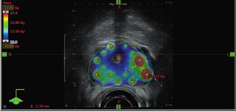
Figure 2.1 illustrates how a two-dimensional cross section of the structures
of interest related to prostate cancer are delineated on an ultrasound image.
The largest contoured volume, the green contour, is the target (the prostate,
which should be irradiated, including a margin). The urethra is delineated
with a red contour within the prostate. Further, the rectum is the brown
contour below the other structures, at the bottom of the image. The figure also
shows radiation doses in a colour scale, where red indicates a high dose and
blue a lower dose. Dwell positions can be seen as small yellow squares. The
prescription dose is 10 Gy and regions with high doses can be seen surrounding
dwell positions.
The medical images are used to manually contour and define the structures
of interest, which include both the target (tumour, tumours, or other regions
of interest, such as a cavity after surgery which is treated adjuvantly due to
suspected microscopic spread) and OARs in the proximity. There are several
interrelated volume definitions regarding the tumour [9]. First, the gross tu-
mour volume (GTV) contains the region where the tumour has been identified.
Secondly, the clinical target volume (CTV) contains the GTV as well as an
extra margin based on clinical experience and suspected microscopic spread.
Thirdly, the planning target volume (PTV) contains the CTV and possibly
an extra margin because of uncertainties due to movements (e.g. breathing)
or technical reasons. See Figure 2.2 for an illustration of how these definitions
are related. In our presentation, PTV will generally be used to denote the
target. Smaller CTV margins are in general needed in BT (and hence smaller
PTVs), as compared to EBRT, because the organ motion is less problematic
as the radiation sources move together with the irradiated target.
92. Background Figure 2.1: A 2D section through a 3D dose distribution for prostate cancer on an ultrasound image. The structures of interest are delineated: the prostate (large red contour, green contour adds a margin), the urethra (red contour, in the middle of the prostate) and the rectum (brown contour, below the prostate). The radiation doses are shown in colours, where red indicates a high dose while blue indicates a lower dose, as shown on the scale in the top left corner. Figure 2.2: The relations between the various volume definitions for the target. Dose planning The clinical process around the dose planning is rigorous [10]. First, the dose plan is prepared by a dosimetrist or a physicist. Secondly, the dose plan is reviewed and approved by the treating oncologist. Finally, a second physicist conducts an independent review and quality control. For prostate cancer treatment, the catheters are inserted invasively, which requires the patient to be anaesthetised (spinal or general). As the dose planning commonly is carried out during the treatment, when the patient is anaesthetised, the time needed for planning is of importance, and should be kept short. An illustration of the clinical process for HDR BT for prostate cancer is shown in Figure 2.3. 10
2.2. Clinical treatment evaluation

                                  anaesthesia

                 I. medical                         III. dose
                                   II. target
                  imaging                              and
                                  and organ
                   (ultra-                          catheter
                                  contouring
                   sound)                           planning

                                                       VI.
                     IV.                           treatment
                                    V. dose
                  catheter                          delivery
                                  adjustment
                  insertion                          with an
                                                   afterloader

Figure 2.3: Illustration of the clinical workflow for prostate cancer. The steps
in the upper part of the figure are related to the planning phase and the steps
in the lower part are related to the delivery phase. During all these steps the
patient is under some form of anaesthesia.

    The dose planning has traditionally been conducted with forward planning,
which is a manual iterative process where the dwell times are adjusted until
the treatment goals are achieved, and the planner is satisfied. This can be
time-consuming, with observed planning times of more than 30 minutes [11],
or in the range 20 − 35 minutes [12]. Forward planning is generally performed
in a treatment planning system (TPS), with graphical support and other tools
available.
    The alternative method for dose planning is inverse planning. Here, the
starting point is instead the goals of the treatment and a dose plan that
achieves these goals (at least approximately) is generated. Because of the
computational complexity, the use of optimization models and algorithms are
fundamental for obtaining dose plans by inverse planning.

2.2 Clinical treatment evaluation
We have discussed the decisions of the dose planning problem, which are the
catheter placement, how many catheters to use and where to place them, and
the dwell times. When these decisions have been made, the resulting dose
distribution can be calculated. Two relevant questions are now (i) how to
evaluate the result, and (ii) which properties of a dose distribution are sup-
ported in the clinical treatment guidelines? In a mathematical optimization

                                                                             11
2. Background
context these questions correspond to how to formulate the objective function
(or functions) and constraints in a dose planning model?
This section is organised as follows. First, the concept of dose points is
introduced, and then we present and discuss several concepts that are used to
evaluate dose plans. This section is based on the presentations in the licentiate
thesis [1] and Paper D.
Dose points and dose calculation
The structures of interest are discretised into dose points, with each dose
point corresponding to a small volume, such as a cube with sides of 1–3 mm.
Clinical treatment guidelines of HDR BT for prostate cancer [10] suggests
that the number of dose points should be at least 5 000 for each structure.
The correlation between the number of dose points and the uncertainty in
evaluation criteria is studied in [13]. For each target and OAR they suggest
32 000 and 256 000 dose points, respectively.
To calculate the dose at any dose point in the patient anatomy, the dose-
rate contribution per second from each dwell position is needed. The calcula-
tions of the dose-rate contributions are today generally based on the AAPM
TG43 formalism [5, 14, 15], by which the composition of the patient is ap-
proximated by water. This approximation is considered good enough for most
applications using the common HDR BT isotope 192 Ir. The water approxima-
tion is less accurate for the isotope 169 Yb, since it has a lower photon energy.
For IMBT applications, where high-Z shields are present within the applica-
tors, model-based dose calculations [16] are used, taking the source model,
the patient geometry and the shields into account [6].
The dose at any dose point can be calculated by summing the dose contri-
butions from all dwell positions, which is the dwell time in seconds multiplied
by the dose-rate contribution. Finally, the dose is scaled with respect to the
strength of the radiation source, which depends on its daily air kerma strength
[14], which decays according to the half-life of the isotope.
Dose-volume histogram
In a dose-volume histogram (DVH), portions of a structure are plotted against
dose levels. The DVH is a convenient way to visualise the dose distribution,
and it is routinely used in clinical dose planning. DVHs can be presented
in a differential or cumulative version. The differential shows, for each dose
level, the portion that receives (within an interval) that dose (in Gy), while
the cumulative shows, for each dose level, the portion that receives at least
that dose; see Figures 2.4 and 2.5 for examples of differential and cumulative
DVHs, respectively. In this presentation, the term DVH refers to the more
commonly used cumulative DVH (unless otherwise specified).
122.2. Clinical treatment evaluation
To compare different DVHs, values at specific points on the curves are
of interest; such values are referred to as dosimetric indices (DIs), for which
there are two formulations. These are referred to as volume-at-dose, denoted
Vxs , or dose-at-volume, denoted Dys , respectively. The same notation as in
Paper D is used here, where x is a dose level, s is a structure, either PTV or
part of the PTV, or an OAR, and y is a portion or a volume (commonly in
cubic centimetres, cc) of structure s. The DI Vxs is the portion of the structure
that receives at least the specified dose level x, while the DI Dys is the lowest
dose in either the portion or the volume, of size y, that receives the highest
dose. If no structure is specified for a DI, it refers the PTV. For comparison
of DIs which are calculated on different systems, it is important to be aware
of that actual values depend on factors such as image slice thickness and the
TPS implementation of volume interpolation, see [17].
volume (%)
dose (Gy)
Figure 2.4: Example of a differential DVH.
volume (%)
y
Vxs
Dys x dose (Gy)
Figure 2.5: Example of a cumulative DVH.
132. Background
Dose homogeneity and conformity
Conformity measures are used to quantify how well the prescription dose
conforms to the target. Homogeneity measures instead quantify how homo-
geneous the dose is within the target. The notation here is the same as in
Paper D.
A homogeneity measure that uses two specified points on the DVH is the
dose homogeneity index (DHI) [18], which is defined as
PTV
V100 − V150
PTV
DHI = PTV
, (2.1)
V100
where 100 and 150 are percentages of the prescription dose. The DHI takes
a value in the range zero to one; the value one is considered ideal, and corre-
sponds to all dose points receiving a dose between the prescription dose and
150% of the prescription dose.
A proposed conformity measure is the conformation number (CN) [19]. In
addition to the dose to the PTV, the portions of the OARs that receive doses
above the prescription dose are also considered. This measure is defined as
P T Vref
CN = V100
PTV
⋅ , (2.2)
T otref
PTV
where P T Vref corresponds to V100 but is expressed as a volume instead of
as a portion, and T otref is the total volume of the structures of interest (with
both PTV and OAR included) which receives at least the prescription dose.
An extension of the CN is the conformal index (COIN) [20], which has an
extra OAR-specific component. The conformal index is calculated as
P T Vref
COIN = V100
PTV
⋅ ⋅ ∏ (1 − V100
s
), (2.3)
T otref s∈SO
where SO is the set of OARs. Both CN and COIN take a value between zero
and one, with one being the best possible value in both measures; for both
measures, this corresponds to the whole PTV receiving the prescription dose
and no portion of any OAR receiving a higher dose than the prescription dose.
Reviews of conformity and homogeneity measures can be found in [21] and
[22].
Radiobiological concepts
The previously introduced evaluation criteria, DIs and homogeneity and con-
formity measures, are based solely on the physical doses. Another principle for
dose plan evaluation is based on radiobiological models, giving criteria meant
to explicitly quantify the radiobiological treatment effect of a dose distribu-
tion. The tumour control probability (TCP) is formulated to be an estimate
142.2. Clinical treatment evaluation
of the probability of local tumour control, that is, that there are no surviving
cancer cells in the tumour.
The following is an example of the calculation of a TCP, as given in [23],
⎡ ⎤n
⎢ (S(t)e(b−d)t ) ⎥
⎢ ⎥
T CP (t) = ⎢1 − ⎥ , (2.4)
⎢ (1 + bS(t)e (b−d)t t ′ ⎥
⎢ ′ )⎥
dt
⎣ ∫0 ′
S(t )e (b−d)t
⎦
where t is a time, T is the duration of the treatment, S(t) is the probability
for a cell surviving until time t, n is the initial number of tumour cells, while
b and d are birth and death rates for cells, respectively. As can be seen in
equation (2.4) there are several parameters that must be estimated. The use
of TCP and radiobiological models is discussed in [24].
For an OAR the corresponding radiobiological index is the normal tissue
complication probability (NTCP), which estimates the risk for complications;
see [25] for a summary of how NTCP is modelled and used. The measure
p+ [26] can be seen as a combination of TCP and NTCP, and it estimates the
probability of tumour control without any severe OAR complications.
Another proposed radiobiological measure is the equivalent uniform
dose (EUD) [27]. The single EUD value is the homogeneous dose which would
give the same treatment effects on a tumour as the evaluated inhomogeneous
dose distribution. Hence, it can be used to compare the radiobiological treat-
ment effect from different dose distributions. The EUD has been extended
to the generalized EUD (gEUD) [28], which can be used also for OARs. One
way to define the gEUD is given in [29] as
1/a
1 n
gEU D = ( ∑ Dosei )
a
, (2.5)
n i=1
where n is the number of dose points in the structure considered, Dosei is
the dose at dose point i, and a is a parameter for radiosensitivity, which
depends on the considered structure. The gEUD is easier to calculate than
TCP and NTCP, and has fewer parameters, in equation (2.5) only one, but
it is supposed to capture all structure specific characteristics.
Clinical treatment guidelines
There are established guidelines which are specific for different treatment sites.
Guidelines for HDR BT prostate cancer treatment [10, 30, 31] include planning
aims for the PTV and OARs, expressed in terms of DIs. For example, the
DI V100 should be at least 90% with the additional recommendation to aim
for 95% [10]. The guidelines [31] also recommend reporting a homogeneity
measure which is equivalent to the DHI, see equation (2.1).
There are established clinical BT treatment guidelines also for other treat-
ment sites and cancer diagnoses; see for example the guidelines for vaginal
152. Background cancer [32], cervical cancer [33], head and neck cancer [34], and breast cancer [35]. 16
CHAPTER          3
                                         Dose planning

In this chapter we discuss dose planning from the point of view of mathemat-
ical optimization. The dose planning problem is here defined as either the
decisions of both catheter placement and dwell times, or only the decisions on
dwell times. The catheter placement problem includes how many catheters
to use and where to place them. In dose planning models, the decisions on
where to place the catheters are typically modelled with binary variables for
the available positions, while the dwell times are modelled as continuous non-
negative variables.
    A general multi-objective problem formulation for the full dose planning
problem, including both catheter placement and dwell times, is as follows

                   min fp (D),                               ∀p,            (3.1)
                 gr (D) ≤ 0,                                 ∀r,            (3.2)
                       tj ≤ M z k ,                 j ∈ C , ∀k,
                                                         k
                                                                            (3.3)
                  ∑ zk ≤ N,                                                 (3.4)
                   k
                       Di = ∑ dij tj ,                       ∀i,            (3.5)
                             j

                       zk ∈ {0, 1},                          ∀k,            (3.6)
                       tj ≥ 0,                               ∀j,            (3.7)

where fp (D) denotes an objective function p, D is the vector of doses Di , each
of which is the dose at dose point i, and functions gr denote constraints, one
for each r, in which the doses D are evaluated. Further, the variable tj is the
dwell time at position j, dij is the dose-rate contribution from a dwell position
j to a dose point i, C k is all dwell positions in catheter k, N is the maximal

                                                                              17
3. Dose planning
number of catheters allowed, and the binary variable zk is one if catheter k is
inserted, and zero otherwise.
Constraints (3.3) ensure that only dwell positions in inserted catheters
are active (non-zero), and the constraint (3.4) ensures that the number of
catheters does not exceed the maximal possible number. For the dose planning
models proposed in the literature it is common that the catheter placement
is not considered, that is, the catheter variables zk are fixed a priori to either
zero or one. This is the case for all models introduced in Chapters 4 and 5.
To explain the construction of the dose planning model we use a simplified
example in Figure 3.1. It represents a case of prostate cancer, but only in two
dimensions. There is one binary variable for each catheter, and it is linked to
the dwell time variables; the dwell times in a catheter can be non-zero only
if the binary catheter variable is equal to one. Generally, both the objectives
(3.1) and constraints (3.2) are based on an evaluation of the doses at the
defined dose points in a structure. The objective functions and constraints
can be based on criteria from the clinical treatment guidelines, approximations
thereof, or other properties which are considered beneficial; such examples are
given in Section 2.2.
Figure 3.1: A simplified example of a 2D slice and the relevant concepts for
dose planning. The large ellipse depicts the tumour and the smaller grey
circle in the middle depict an OAR. The two pairs of vertical lines are the
two possible catheters, and the grey dots are the possible dwell positions with
dwell time variables. The small dots are the dose points, at which the doses
are calculated and evaluated.
3.1 Multi-objectivity
Equations (3.1)–(3.7) state a generic problem formulation, with variables for
which catheters to use and for the dwell times. When the catheter variables
are fixed, it is still a multi-objective formulation because there are multiple
aims for the target (or targets) to which we want to give a radiation dose that
183.2. Why use optimization?
is high enough, and for the OARs to which we want to avoid or limit the dose.
Furthermore, some of these aims are typically in conflict.
In practice, the multi-objective aspect of the dose planning problem is com-
monly handled either by considering a weighted sum of the objective functions
or by considering all but one of the objectives as constraints, keeping only a
single objective in the objective function. All the models presented in Chap-
ter 4, and in Papers A, B, C, and E are single-objective models. There are
several truly multi-objective approaches in the literature, see Paper D for an
overview of such.
In single-objective models the dose planning results in a single dose plan
and, hence if the planner is not satisfied, trade-offs and priorities are han-
dled by changing weights for the objectives or parameters in the objectives
or constraints. True multi-objective approaches however result in a number
of solutions which the planner can choose from. The necessary trade-offs be-
tween conflicting aims can thus be made clear. Both the tasks of solving
single-objective models repeatedly (if necessary) and navigating a number of
solutions from a multi-objective approach can be time consuming.
The dose planning problem is approached quite differently in the proposed
models in the literature, with different types of criteria included and different
types of models. Nevertheless, dose plans which are clinically acceptable can
be obtained from various approaches, possibly including parameter tuning.
3.2 Why use optimization?
There are important advantages with the use of mathematical optimization
for dose planning. First, it is possible to save time in the treatment plan-
ning process. This is especially important when the patient is under some
form of anaesthesia during the dose planning. Optimization methods for dose
planning have been reported to only take a few seconds, see for example [11,
36], and most approaches do not require more than a few minutes to find
acceptable dose plans. Secondly, several studies have shown improvements in
dose plan quality compared to manual planning; see [11, 36, 37, 38, 39, 40] for
prostate cancer examples. Furthermore, the use of mathematical optimization
also reduces the dependence of personnel skills and experience on treatment
outcome.
The emerging treatment modality IMBT puts additional demands on
mathematical optimization approaches because of the additional degrees of
freedom introduced by the shields. These additional degrees of freedom clearly
also make manual planning of IMBT much harder than of conventional HDR
BT.
19CHAPTER 4
Mathematical models for
dose planning
In this chapter we introduce three well-studied models for dose planning.
These are used or further studied in Papers A, B, C, and E. The model
formulations and illustrations are based on the licentiate thesis [1] and the
literature review Paper D, which is further discussed in Chapter 5.
Table 4.1 introduces the notations in common for the models. A subscript
or superscript O refer to an OAR, and T refers to the PTV, which here is
a single volume as is typically the case for prostate cancer. (The presented
optimization models can easily be generalised to the case with several PTVs.)
The set S contains all structures of interest, including both the PTV and
OARs. The mathematical models use pre-calculated dose-rate contributions,
denoted dij , where i is a dose point and j is a dwell position.
4.1 Linear penalty models
An optimization model for dose planning which is commonly used in clinical
practice is simply based on penalties to the dose points whose doses are outside
specified intervals. There is no penalty when the dose is within the specified
interval, and outside this interval the penalty increases linearly. The objective
function is to minimise the total sum of penalties. Such a model is referred
to as the linear penalty model (LPM). A tailored meta-heuristic method for
solving the LPM, for HDR BT, called inverse planning simulated annealing
(IPSA), was proposed in [41]. (See e.g. [42] for a description of simulated
annealing.) The LPM was in [43] formulated and solved as a linear program
(LP), which made it possible to find and prove a globally optimal solution.
214. Mathematical models for dose planning Table 4.1: Indices, sets, parameters and variables in common for the opti- mization models; the notations are taken from [1]. Indices i Index for a dose point j Index for a dwell position s Index for a structure Sets S Set of structures, including PTV and OARs SO Set of OARs, including an artificial structure of healthy tissue, SO ⊂ S Ps Set of dose points in structure s ∈ S P Set of all dose points, P = ∪s∈S Ps PT Set of dose points in the PTV J Set of dwell positions Parameters dij Dose-rate contribution from dwell position j ∈ J to dose point i ∈ P Ls Prescription dose or a lower dose bound for structure s ∈ S Us Upper dose bound for structure s ∈ S Ms Maximum allowed dose for structure s ∈ S wsl Non-negative penalty for dose being too low in structure s ∈ S wsu Non-negative penalty for dose being too high in structure s ∈ S Variables Dosei Dose at dose point i ∈ P tj Dwell time for dwell position j ∈ J xli Penalty variable for dose being too low at dose point i ∈ Ps , s ∈ S xui Penalty variable for dose being too high at dose point i ∈ Ps , s ∈ S Another linear penalty model has been proposed [44], in which the maximum deviation from the specified dose intervals is minimised. Table 4.1 introduces the notation used for the LPM. 22
4.1. Linear penalty models

   By definition, xli = max{Ls − ∑j∈J dij tj , 0} and xui = max{∑j∈J dij tj −U s , 0}
shall hold. In the LPM, these relations are modelled with linear constraints.
The LPM is mathematically formulated as follows.

                        min ∑ wsl ∑ xli + ∑ wsu ∑ xui                         (4.1a)
                                   s∈S   i∈Ps   s∈S   i∈Ps

                 subject to
                  ∑ dij tj ≥ L − xi                    i ∈ Ps , s ∈ S
                              s   l
                                                                              (4.1b)
                  j∈J

                  ∑ dij tj ≤ U + xi                    i ∈ Ps , s ∈ S
                              s   u
                                                                              (4.1c)
                  j∈J

                        xli ≥ 0                        i ∈ Ps , s ∈ S         (4.1d)
                        xui   ≥0                       i ∈ Ps , s ∈ S         (4.1e)
                        tj ≥ 0                                 j∈J            (4.1f)

Constraints (4.1b) and (4.1d), together with the minimisation in the objective
function ensure that xli = max{Ls − ∑j∈J dij tj , 0} holds in an optimal solution.
Constraints (4.1c) and (4.1e) works similarly, but for the upper dose bound
penalty variable.
    In the LPM there are no constraints that define feasibility from a clini-
cal point of view. Hence, each choice of non-negative dwell times, tj , j ∈ J,
corresponds to a feasible solution in the model. Because the penalty param-
eters have no direct clinical interpretation and the clinical evaluation criteria
are not included explicitly in the model, tuning of the penalty parameters is
generally needed to obtain clinically acceptable dose plans. Thus, although
computing times for solving the model are short, the overall process of dose
planning can be time consuming.
    The objective function value of the LPM has no clinical meaning in itself,
and to evaluate solutions, criteria from the clinical treatment guidelines, such
as the dosimetric indices, are used. Furthermore, it has been observed that
dose plans can have equal LPM objective function values but differ in DIs,
or vice versa. Such an example can be found in [45], in which two similar
plans differed with a factor of 12 in terms of LPM objective value. This was
also observed in [43] where solutions obtained with IPSA were compared with
solutions obtained from the LPM. Although the LPM objective function value
was improved significantly, this was not reflected by the DIs.
    Dose plans obtained from the LPM have also been analysed with respect to
other properties. Dwell times obtained from the LPM were in [46] compared
to dwell times from manual dose plans and found to be less homogeneous.
The inhomogeneous dwell times were further studied in [47], and shown to be
an inherent property of the model.
    A convex piecewise linear penalty model was proposed in [47], to obtain
dose plans with more homogeneous dwell times. The piecewise linear penalty

                                                                                  23
4. Mathematical models for dose planning
model was shown to produce dose plans with more homogeneous dwell times,
compared to the LPM [47].
The LPM can also be extended with quadratic penalty terms. Quadratic
penalty models are common in conventional HDR BT studies [48, 49] as well
as in IMBT studies [50, 51]. Examples of a linear penalty function, a convex
piecewise linear penalty function, and a piecewise quadratic penalty function
can be seen in Figure 4.1.
penalty
Ls Us dose (Gy)
Figure 4.1: The solid line is a linear penalty function for one dose point. The
dotted line is a piecewise linear penalty function, here with six segments (in-
cluding the horizontal segment). The dashed function is a piecewise quadratic
penalty function.
4.2 Dose-volume models
In dose planning with the LPM, dosimetric indices are only considered af-
terwards, as they are used to decide whether a dose plan is good enough or
not. A more direct approach is to explicitly model DIs in the optimization
model; we refer to this approach as a dose-volume model (DVM). The first
optimization model for HDR BT which included an explicit DI constraint was
proposed and studied in [52]. This model extended an LPM with one DI
constraint, for an OAR. See [45, 53, 54], and Paper B for more examples of
proposed DVMs.
The concept of DIs can be found in other fields of research. In finance
the counterpart is called value-at-risk (VaR) [55], and a similar construction
is also used in the field of chance constraints [56].
Tables 4.1 and 4.2 introduce the notation used for the DVM. The following
mixed-integer programming (MIP) DVM model is adapted from [53] and [54],
and uses the same notation as in [1] and Paper D.
244.3. Mean-tail-dose models
Table 4.2: Notation used for the dose-volume model.
Parameters
τ s Portion of a structure, here used for OAR s ∈ SO
Variables
yi Binary indicator variable for PTV dose points, i ∈ PT , that takes the value one
if the dose is at least LT , and zero otherwise
vis Binary indicator variable for OAR dose points, i ∈ Ps , s ∈ SO , that takes
the value one if the dose is at most U s , and zero otherwise
1
max ∑ yi (4.2a)
∣ PT ∣ i∈PT
subject to
∑ dij tj ≥ L yi i ∈ PT
T
(4.2b)
j∈J
∑ dij tj ≤ M − (M − U )vi i ∈ Ps , s ∈ SO
s s s s
(4.2c)
j∈J
∑ vi ≥ τ ∣ Ps ∣ s ∈ SO
s s
(4.2d)
i∈Ps
yi ∈ {0, 1} i ∈ PT (4.2e)
vis ∈ {0, 1} i ∈ Ps , s ∈ SO (4.2f)
tj ≥ 0 j∈J (4.2g)
The notation ∣ Ps ∣ is used for the number of dose points in structure s. The
objective is to maximise V100 , which corresponds to maximising the number
of PTV dose points at which the dose is high enough, expressed via the binary
indicator variable yi . Constraints (4.2b) ensure that each yi takes the correct
value, that is, one if the dose is not below the prescription dose LT and zero
otherwise. The combination of constraints (4.2d) and (4.2c) ensures that the
constraints on DIs for OARs are satisfied. Constraints (4.2c), belong to a
type of constraints which are commonly referred to as “Big-M” constraints.
These constraints impose a strict upper bound, M s , on the dose at each dose
point. The value of M s can be set to a clinically relevant value, if available,
or otherwise to a value which is large enough to not cut away any feasible
solution.
4.3 Mean-tail-dose models
The conditional value-at-risk (CVaR) is a financial risk measure which has
been used also in radiation therapy. In finance, CVaR is the mean value of
25You can also read