Short-Term River Flood Forecasting Using Composite Models and Automated Machine Learning: The Case Study of Lena River
←
→
Page content transcription
If your browser does not render page correctly, please read the page content below
water
Article
Short-Term River Flood Forecasting Using Composite Models
and Automated Machine Learning: The Case Study of
Lena River
Mikhail Sarafanov * , Yulia Borisova *, Mikhail Maslyaev, Ilia Revin, Gleb Maximov                                 and Nikolay O. Nikitin

                                          National Center for Cognitive Research, ITMO University, 49 Kronverksky Pr., 197101 Petersburg, Russia;
                                          mikemaslyaev@itmo.ru (M.M.); ierevin@itmo.ru (I.R.); gimaksimov@itmo.ru (G.M.); nnikitin@itmo.ru (N.O.N.)
                                          * Correspondence: mik_sar@itmo.ru (M.S.); jul.borisova@itmo.ru (Y.B.)

                                          Abstract: The paper presents a hybrid approach for short-term river flood forecasting. It is based
                                          on multi-modal data fusion from different sources (weather stations, water height sensors, remote
                                          sensing data). To improve the forecasting efficiency, the machine learning methods and the Snowmelt-
                                          Runoff physical model are combined in a composite modeling pipeline using automated machine
                                          learning techniques. The novelty of the study is based on the application of automated machine
                                          learning to identify the individual blocks of a composite pipeline without involving an expert. It
                                          makes it possible to adapt the approach to various river basins and different types of floods. Lena
                                          River basin was used as a case study since its modeling during spring high water is complicated by
                                          the high probability of ice-jam flooding events. Experimental comparison with the existing methods

                                   confirms that the proposed approach reduces the error at each analyzed level gauging station. The
                                          value of Nash–Sutcliffe model efficiency coefficient for the ten stations chosen for comparison is 0.80.
Citation: Sarafanov, M.; Borisova, Y.;
                                          The other approaches based on statistical and physical models could not surpass the threshold of 0.74.
Maslyaev, M.; Revin, I.; Maximov, G.;
                                          Validation for a high-water period also confirms that a composite pipeline designed using automated
Nikitin, N.O. Short-Term River Flood
Forecasting Using Composite Models
                                          machine learning is much more efficient than stand-alone models.
and Automated Machine Learning:
The Case Study of Lena River. Water       Keywords: flood forecasting; automated machine learning; composite artificial intelligence
2021, 13, 3482. https://doi.org/
10.3390/w13243482

Academic Editors: Zheng Duan              1. Introduction
and Babak Mohammadi                       1.1. Modelling of the River Floods
                                               River floods can be considered as a crucial type of dangerous event. The damage
Received: 9 November 2021
                                          caused by a river flood may reach hundreds of thousands of dollars [1,2]. Moreover, natural
Accepted: 3 December 2021
                                          hazards take lives and affect a large number of people every year [3]. Because it is vital to
Published: 7 December 2021
                                          predicting such floods successfully, there are a lot of scientific works dedicated to flooding
                                          operational modeling based on various solutions [4].
Publisher’s Note: MDPI stays neutral
                                               To reduce the damage caused by natural disasters, forecasting systems are used.
with regard to jurisdictional claims in
                                          They are based on models that predict water levels and flow rates. Classical methods
published maps and institutional affil-
iations.
                                          used in hydrology are based on determining the dependence between meteorological
                                          data, basin and substrate characteristics, and modeled target values [5]. There are widely
                                          used approaches to modeling nature processes, which were implemented in the form of
                                          hydrological models. Such models mainly rely on the deterministic approach, but some
                                          models operate with elements of stochastic nature [6]. It allows us to reproduce a wide class
Copyright: © 2021 by the authors.
                                          of processes with suitable hydrological models. The advantage of such models is that they
Licensee MDPI, Basel, Switzerland.
                                          are can be well interpreted by experts [7]. Most models are not implemented for a specific
This article is an open access article
                                          region but represent the bonds between the components of almost any river system.
distributed under the terms and
conditions of the Creative Commons
                                               Model calibration is used to take into account the specific characteristics of a particular
Attribution (CC BY) license (https://
                                          region [8]. Adapting the model to the desired domain allows reducing forecast error.
creativecommons.org/licenses/by/          However, for complex models, calibration can be too complicated and computationally
4.0/).                                    expensive. Moreover, complex physical models require a lot of data that may not exist or

Water 2021, 13, 3482. https://doi.org/10.3390/w13243482                                                     https://www.mdpi.com/journal/water
Water 2021, 13, 3482                                                                                          2 of 28

                       may not be insufficient quantity for the modeled river basin. Due to the difficulties with
                       calibration, the application of such models becomes inefficient in some cases [9].
                             Another way of physical modeling for flood prediction is explaining flow patterns
                       through differential equations. The disadvantages of the equation-based models are
                       the unstable solutions caused by errors accumulation [10] and high computational and
                       algorithmic requirements. Moreover, such approaches may be challenging to generalize to
                       other rivers and basins, for which they require the addition of new parameters.
                             To take local effects into account, data-driven approaches based on machine learning
                       (ML) methods can be used [11]. They are less interpretable but can produce high-quality
                       forecasts [12]. On the other hand, complex machine learning models, such as neural
                       networks, require a lot of data to train.
                             To account for the advantages of physical models (interpretability) and machine
                       learning models (low forecasting error), ensembling is used [13]. Such hybrid models
                       allow for a refinement of predictions derived from hydrological models [14] using ML
                       techniques. To improve such multi-level forecasting models data fusion methods [15] can
                       be used. Such approaches based on the ensemble of different models (machine learning-
                       and physics-based) are becoming more popular in the design of predictive systems. Also,
                       the perspective approach that allows to train and calibrate models differently for each data
                       source can be proposed. In that case, distortions and errors in one source cannot lead to
                       critical errors in the whole system [16]. Unfortunately, such complex hybrid pipelines are
                       hard to identify and configure.
                             To simplify the identification task, automated machine learning (AutoML) can be
                       applied. Methods and algorithms of AutoML are devoted to automated identification
                       and tuning of ML models. A main concept of the AutoML approach is the building of
                       ML models without the involvement of an expert or with their minimal involvement.
                       However, most of the existing AutoML tools cannot be used to obtain heterogeneous
                       (composite) pipelines, that combined models of different nature (for example, ML models
                       and hydrological models). At the same time, composite modeling is especially promising
                       for flood forecasting since it allows combining the state-of-the-art data-driven and physics-
                       based methods and models according to the Composite Artificial Intelligence concepts [17].
                             In the paper, we propose an automated approach for short-term flood forecasting.
                       The approach is based on the application of automated machine learning, composite mod-
                       els (pipelines), and data fusion. Application of the various data sources (meteorological,
                       hydrological, and remote sensing measurements) in combination with automated identi-
                       fication and calibration of the models make it possible to construct composite pipelines.
                       Machine learning methods are used to forecast time series of daily water levels. Short-
                       term prediction of this variable allows us to avoid negative effects from its rapid increase
                       through prompt decision-making. Involvement of the physical models allows improving
                       the interpretability of the final pipeline. This solution can be used for the analysis of the
                       river’s condition.

                       1.2. Existing Methods and Models for Flood Forecasting
                             In this subsection we are analyzing the most significant causes of floods and the
                       specific features of the Lena River basin, which do not allow to apply of existing approaches
                       for flood modeling in this area.
                             Siberia region floods are of interest to researchers because of their destructive power
                       and annual occurrence [18,19]. Regarding the Lena River, its condition has been studied
                       and modeled by researchers as classical methods of expert search for dependencies between
                       the components of the system [20] as numerical methods. Because the river flows in a cold
                       climate, most of the year channels are covered with ice and snow. So numerical models for
                       this region are created to assess both ice conditions [21] and channel changes during the
                       ice-free period [22].
                             The major difficulty in modeling floods on the Lena river is in a high variety of flood
                       causes. The largest floods occur when the superposition of several factors of water level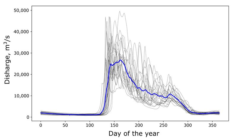
Water 2021, 13, 3482                                                                                                          3 of 28

                                rise at once: a regular rise associated with melting snow in spring and extreme rises in from
                                ice-jam. It is difficult to predict such floods on the basis of snowmelt or on retrospective
                                statistical information alone.
                                      Based on an extensive literature review [23], we can consider the following causes of
                                river flooding (most relevant for the Lena river):
                                •       Floods caused by heavy rainfall [24];
                                •       Floods due to melting snow [25];
                                •       Surges from the sea [26];
                                •       Extreme rises in water levels due to ice jams, debris flows, rocks blocking the riverbed,
                                        etc. [27,28];
                                •       A combination of several factors.
                                     For the Lena River basin, flooding in the spring period is most typical due to snow
                                melting, precipitation and a high probability of ice-jam formation [28]. The following ways
                                of modeling each type of flood are presented in Table 1.
      Table 1. Methods and models for flood forecasting. The “Flood type” column shows the flood factors that the model is
      capable of incorporating.

           Model                 Description                  Advantages                 Limitations             Flood Type
                                                                                         Only rainfall
        Deep neural             Based only on                  Few data
                                                                                           flood can              Rainfall
       network [29,30]          seasonal data                 are required
                                                                                         be simulated
         Hybrid ML
                                  Determing                  Less prediction
           (ANN                                                                          Only rainfall
                                  dependence                   error than
            and                                                                            flood can              Rainfall
                                 from rainfall                stand-alone
          K-nearest                                                                      be simulated
                                 and time step                   models
       neighbors ) [31]
                                Based on flow                                               Short
                                                                Relatively
          Wavelet                   and                                                   (1–2 days)              Rainfall,
                                                                   low
        analysis [32]           meteorological                                             forecast              Snowmelt
                                                              forecast error
                                 time series                                               horizons
                                   Transform
         Snowmelt               snowmelt and               Reliable model [34],            Requires
                                                                                                                  Rainfall,
          Runoff                rainfall water                   detailed                  accurate
                                                                                                                 Snowmelt
         model [33]              into the daily              user’s manual               snowfall data
                                   discharge
                                Calculation of
           System                  vertical                                             Large amount
                                                             Relatively low                                       Rainfall,
          dynamics              water balance                                               of data
                                                             forecast error                                      Snowmelt
        approach [35]             based on                                               are required
                                  storages
        Precipitation
                                Modeling based                                          Large amount
           Runoff                                                Detailed                                         Rainfall,
                                 on physical                                                of data
         Modeling                                             user’s manual                                      Snowmelt
                                  equations                                              are required
        System [36]
                                Ice dynamics
                                                             High temporal              Large amount
                                and hydraulic                                                                    Snowmelt,
         RIVICE [37]                                         sampling rate                  of data
                                  processes                                                                       Ice-jam
                                                             for simulation              are required
                                 calculation
                                                                                          Inability to
                                                                                             model
                                    Time series
         AR [38],                                              Few data                    nonlinear
                                    forecasting                                                                   Common
        ARIMA [39]                                            are required                 processes,
                                      models
                                                                                           relatively
                                                                                        “weak” models

                                     As can be seen from the table, there are several approaches that can be suitable for
                                Lena River floods forecasting. Nevertheless, each of them has disadvantages that do not
                                allow to use of only one method. Therefore, we decided to build a composite model
                                (pipeline) based on several blocks. Each of the individual blocks is modeling the desired
                                component of the flood.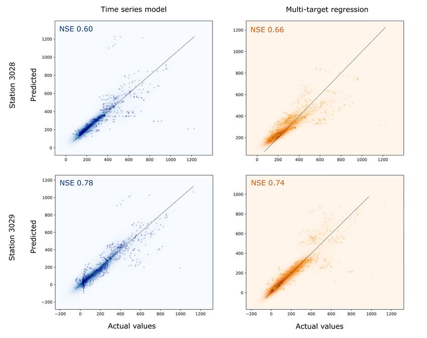
Water 2021, 13, 3482                                                                                            4 of 28

                             It is worth adding that the frequency of occurrence of each cause is different [40]. The
                       rise in water levels associated with melting snow can be attributed to regular (annual)
                       phenomena. At the same time, conditions associated with high precipitation and the
                       formation of ice jams are non-periodic. Such causes are highly dependent on the synoptic
                       situation in the region. In addition, the precipitation field is spatially heterogeneous,
                       which makes it impossible to predict the average increase in water at all hydro gauges.
                       Precipitation may cause localized increases in water levels in some parts of the river due to
                       different rainfall intensities and soil characteristics. The same problem exists for ice-jam
                       floodings. The rise of the level at a specific level gauge not always leads to an increase in
                       the level at the neighboring ones. So, it becomes extremely important to consider local
                       features not only for the basin but for specific sections of the river and watersheds.
                             The second important factor is the remoteness of the Lena River from major cities. The
                       river basin is very large, and at the same time, the number of hydro gauges is not high
                       enough. For this reason, the models that are based on remote sensing data are often used for
                       flood forecasting on the Lena River [41]. A widespread method is the application of models
                       or manual interpretation to remote sensing data for the tasks of detecting and predicting
                       river spills. The example is presented in article [42], which demonstrates the calculation
                       of a set of river state parameters, such as discharge, propagation speed, and hydraulic
                       geometry with Moderate Resolution Imaging Spectroradiometer (MODIS) satellite imagery.
                       Also, Landsat satellite images were used for monitoring the spatial and temporal extent
                       of spring floods [43] on the Lena River. Also, remote sensing data are calibrated with in
                       situ observations [44,45], which allows supplementing the data. The context of such works
                       implies the detection of the current state of the river. The emphasis on predictive models is
                       usually not made. Numerical models allow reproduction of the state of a watercourse at
                       any period of time, based on some input set of actual data.
                             We can conclude that the rise in water levels in the Lena River depends on many factors.
                       Each of these causes contributes to the overall increase in the level at all hydro gauges on
                       the river, as well as at only some of them. In the paper, we refer to the floods that are caused
                       by a combination of several causes as multi-causes flooding. For example, when the water
                       level rises due to both snow melting and the ice-jams formation. Successfully managing all
                       of these factors requires a comprehensive approach. The described approaches are (1) too
                       complicated to prepare and calibrate, or (2) do not take all crucial flood causes into account.
                       Therefore, in the proposed approach we design an ensemble of several models to combine
                       the advantages of different methods in a single composite pipeline. The novelty of this
                       approach is the automatic identification of individual blocks in the predictive system, as
                       well as the hybridization of models for multi-causes flood forecasting.
                             Each of the individual blocks in the pipeline is designed to predict a flood based on
                       one or several of the described causes. Each block is specialized to reproduce the required
                       patterns from the provided data only. The simulation blocks can be physical models as well
                       as ML models. Since the identification and tuning of ML models requires the involvement
                       of an expert and takes a lot of time, special algorithms for automation are used. The
                       proposed AutoML approach is based on the evolutionary algorithm for identifying ML
                       models. It allows to automatically identify models, tune hyperparameters, and combine
                       stand-alone models into ensembles. Moreover, the optimal ML model structure search
                       process is designed in such a way that can simplify the structure of the pipelines. This
                       allows obtaining stand-alone models as the final solution if that is sufficient for successful
                       forecasting. In addition, modern AutoML solutions have already shown their high accuracy
                       compared to stand-alone models [46]. It also makes the approach more flexible, since
                       identifying individual blocks becomes possible without involving an expert. Consequently,
                       the forecasting system is easier to transfer to new basins and rivers if AutoML algorithms
                       are used.
                             We validated this approach on the Lena River basin. Floods in this territory are an
                       actively and sufficiently studied common occurrence. Such phenomenon is annual and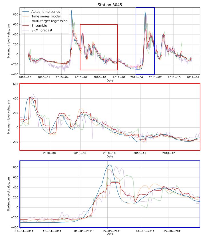
Water 2021, 13, 3482                                                                                            5 of 28

                       directly depends on runoff factors also including ice-jam formations [18]. For this reason,
                       the analysed area is a suitable for the validation of constructing multi-causes flood system.
                            The paper is organized as follows. Section 1 contains the description of the existing
                       approach for flood forecasting. Section 2 described the different aspects of the proposed
                       automated approach and validation methods. Section 3 provides the extensive experimen-
                       tal validation of the proposed approach for the Lena River case study; Section 4 described
                       the main limitation of the study and obtained insight. Finally, Section 5 summarizes the
                       achieved results and provides references to the code and data used in the paper.

                       2. Materials and Methods
                       2.1. Input Data for Case Study
                            The input data for modeling and validation are provided by The Russian Federal
                       Service for Hydrometeorology and Environmental Monitoring and Federal Agency of
                       Water Resources [47,48]. For both physical modeling and the machine learning approach,
                       data from hydro gauges and weather stations were used. Locations of stations and zone of
                       interest are shown in Figure 1.

                       Figure 1. Spatial position of observation stations and Lena River basin.

                             The Lena River is located in Eastern Russia. The area of the basin is 2,430,000 km2 [49].
                       This region can be characterized by a Siberian climate with extremely low temperatures dur-
                       ing winter. The river flows entirely in permafrost conditions [50] from south to north, which
                       is increasing the probability of ice-jam flooding during spring periods [28,51]. As was men-
                       tioned earlier, the following causes of spring floodwater on the Lena River include: [28]:
                       •    Large amounts of precipitation during autumn;
                       •    Low temperatures during winter with extensive accumulation of snow;
                       •    Early prosperous spring with rapid increasing of daily temperature;
                       •    Heavy precipitation during snowmelt.
                           The rise in the water level, as well as the increase in flow, typically occurs during the
                       beginning of May to mid-July (Figure 2).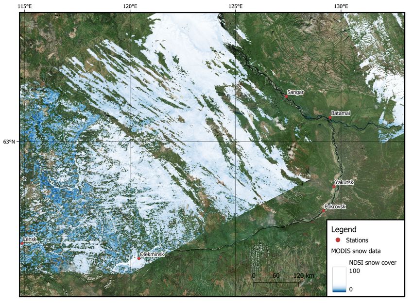
Water 2021, 13, 3482                                                                                                6 of 28

                       Figure 2. Flow graph for “Tabaga” hydro gauge on the Lena River. The blue line shows the average
                       values for the period from 1985 to 2011. The black lines show the values of river flow for specific
                       times each year.

                            The successful prediction of extreme water level rises requires using not only the
                       prehistory of water level but also information from weather stations and date and time
                       values. It is also vital to aggregate the features for the previous periods which show the
                       conditions in which the snow cover formed in the river basin, etc. To get the most complete
                       and operational information about the modeled basin, various data sources (tables, time
                       series, images) were used:
                       •    Water levels at gauging stations in the form of time series with daily time resolution;
                       •    Meteorological parameters measured near the level gauging stations and additional
                            information about the events at the river;
                       •    Meteorological parameters from weather stations. Time resolution for parameters may
                            differ from three hours to daily. This data refers to points located at some distance
                            from level gauging stations;
                       •    Additional information, derived from open sources, such as remote sensing data from
                            MODIS sensor.
                             Parameters that were recorded at the weather stations and hydro gauges are shown in
                       Table 2.
                             Remote sensing data from the MODIS sensor was used as an additional data source
                       to train the physical model. If necessary, interpolation and gap-filling were applied to the
                       values of the meteorological parameters from tables.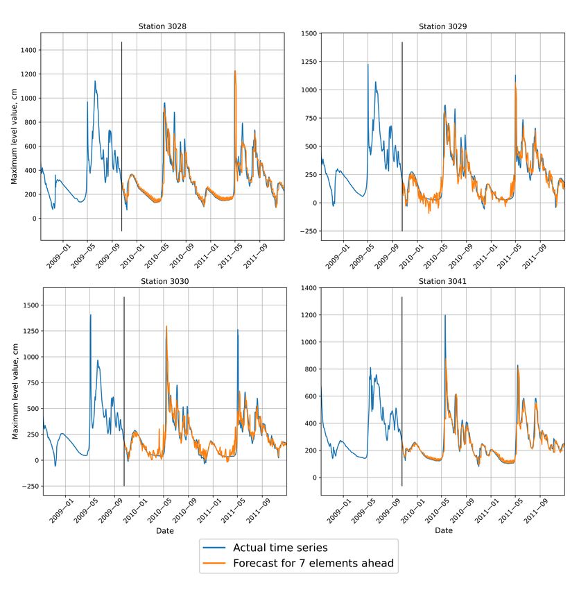
Water 2021, 13, 3482                                                                                                   7 of 28

                       Table 2. Data sources and parameters that were used for fitting and validation of the models.

                                                  Time
                            Data Source                              Parameter                     Description
                                                  Step
                                                                                              Maximum water level
                                                                    stage_max
                                                                                                  per day, cm
                                                                                               Average daily water
                                                                       temp
                                                                                                temperature, ◦ C
                            Hydro gauges           1d                                        Code of events registered
                                                                    water_code
                                                                                                   on the river
                                                                   ice_thickness                 Ice thickness, cm
                                                                                               Average daily water
                                                                     discharge
                                                                                                 discharge, m3 c
                                                                  air_temperature              Air temperature, ◦ C
                                                                 relative_humidity             Relative humidity, %

                                                   3h                                        Atmospheric pressure at
                                                                     pressure
                                                                                                station level, hPa
                           Weather stations                                                   Sum of precipitation
                                                                   precipitation
                                                                                            between timestamps, mm
                                                                                                 Snow coverage of
                                                              snow_coverage_station
                                                   1d                                          the station vicinity, %
                                                                   snow_height                   Snow height, cm

                       2.2. Composite Modelling Approach
                            Composite models (pipelines) show strong predictive performance when processing
                       different types of data [52]. Therefore, to build a precise and at the same time robust model,
                       it was decided to use a composite approach with automatic machine learning techniques
                       and evolutionary computing. Each of the composite pipeline blocks was compiled either
                       completely using automatic model design generation or using optimization algorithms
                       for block (model) calibration. We propose to build a composite flood forecasting model
                       consisting of three blocks:
                       •    Machine learning model for time series forecasting. Predictions of such a model based
                            on time series of water levels. The number of such models equals the number of
                            gauging stations;
                       •    Machine learning model for multi-output regression. Predictions of such a model
                            based on meteorological conditions. The number of such models equals the number
                            of gauging stations;
                       •    Snowmelt-Runoff Model. The physical model is implemented and configured for the
                            most critical level gauges;
                            The target variable for such a system to predict is the maximum daily water level. The
                       configuration of the final model together with the model blocks can be seen in Figure 3.
                            The pipeline presented in Figure 3 allows using as much data as possible. The primary
                       reason to use an ensemble in a composite pipeline is a reduction of forecast error compared
                       to stand-alone models [53]. Also, it allows specialization of individual blocks of the
                       composite ensemble to solve the utilitarian task.
                            As an example, the multi-output regression model predicts water levels based on
                       mostly meteorological data. The time series forecasting model predicts only on the basis of
                       previous level values using autoregressive dependencies. Then, if incorrect values of mete-
                       orological parameters are obtained and the multi-output regression model is producing
                       incorrect forecasts, the time series forecasting model still can preserve the stability of the
                       ensemble. The use of the physical model makes it possible to interpret the forecast.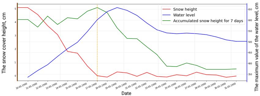
Water 2021, 13, 3482                                                                                               8 of 28

                       Figure 3. Data processing scheme in the composite pipeline. The ensemble consists of three models,
                       each of which is trained and calibrated on separate data source.

                            Therefore, if any of the models produce an unrealistic result, the expert can refer to
                       the snow-melt runoff model on the critical (main) gauging station and check the adequacy
                       of the system output.
                            Another advantage of the composite approach is its robustness - not only to distorted
                       measurements, but also to the lack of data sources. If multiple data sources exist, it is
                       possible to re-configure the pipeline and use the blocks with available input data only.
                            Individual blocks based on machine learning models are identified using the evolu-
                       tionary algorithm for automatic machine learning described in the paper [52]. Then, the
                       ensembling was used to combine the predictions of the individual blocks in the composite
                       pipelines. Most solutions with using model ensembling are aimed at ensuring that the
                       ensemble is “sufficiently diverse”. Therefore, the errors of individual algorithms on par-
                       ticular objects will be compensated for by other algorithms. When building an ensemble,
                       the main task is to improve the quality of modeling of basic algorithms and increasing
                       the diversity of basic algorithms. This effect is achieved through the following methods:
                       changing the volume of the training data set, target vector, or set of basic models. In
                       this paper, the Random Forest model was used as meta-algorithm for ensembling. The
                       predictors were the following: the predictions of the individual blocks, month and day.
                       Next, a general scheme for optimizing the resulting ensemble is applied. The rationale for
                       using the meta-algorithm is the fact that an ensemble can represent a significantly more
                       complex function than any basic algorithm in many cases. So, ensembles allow us to solve
                       complex problems with simple models. The effective adjustment of these models to the
                       data occurs at the level of a meta-algorithm.
                            To find the optimal hyperparameters values for the ensemble model we apply Bayesian
                       optimization [54]. The Bayesian optimization is a modification of random search optimiza-
                       tion. The main idea is to choose the best area of the hyperparameter space, based on
                       taking into account the history of the points at which the models were trained and the
                       values of the objective function were obtained. This hyperparameter optimization method
                       contains two key blocks: a probabilistic surrogate model and an acquisition function for
                       the next point. We can consider this as an ordinary usual machine learning task, where the
                       selection function is a quality function for the meta-algorithm used in Bayesian hyperpa-
                       rameter optimization, and the surrogate model is the model that we get at the output of
                       this meta-algorithm. The widely-used functions are Expected Improvement, Probability
                       of Improvement, and, for surrogate models, Gaussian Processes (GP) and Tree-Structured
                       Parzen Estimators (TPE) [55]. At each iteration, the surrogate model is trained for all previ-
                       ously obtained outputs and tries to get a simpler approximation of the objective function.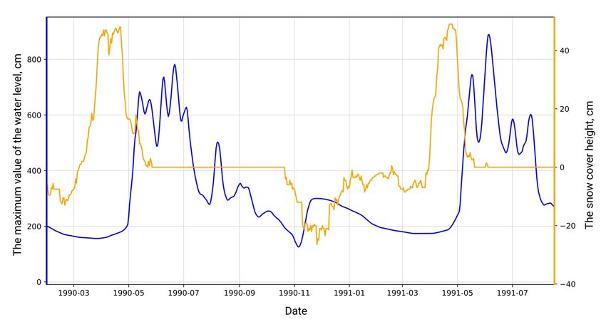
Water 2021, 13, 3482                                                                                               9 of 28

                       Next, the selection function evaluates the “benefit” of the various following points using
                       the predictive distribution of the surrogate model. It balances between the use of already
                       available information and the “exploration” of a new area of space.

                       2.3. Data Preprocessing
                            Qualitative preparation of data before fitting the machine learning models or calculat-
                       ing physical models provides the greatest possibility to improve the result of prediction.
                            As was mentioned before, the primary data set contains observation from two sources:
                       weather stations and hydro gauges, which are located at some distance from each other.
                       The problem can be illustrated by Figure 4. Thereby, some parameters require interpolation
                       to neighboring points for forming the complete dataset for each gauging station.

                       Figure 4. The task of the meteorological parameters values interpolation to the level gauges. The
                       example of mean daily air temperature is presented. Sign “?” means that the value of the parameter
                       in the station is unknown.

                             Even a simple interpolation algorithm can be used to resolve this problem. But there is
                       a need to keep the approach flexible: some weather stations that are close (by longitude and
                       latitude coordinates) to the gauging station can represent the real situation in a non-precise
                       way. It can be caused by topography inhomogeneities.
                             For example, the points are close to each other, but the nearest weather or gauging
                       station is located in the lowlands, and the two neighboring ones are located in the hollows
                       among the ridges. In this case, the best solution would be to take values only from the
                       nearest weather station and not to interpolate at all. In the other case, a good solution
                       would be to average the values from five neighboring weather stations.
                             Bilinear interpolation and nearest-neighbor interpolation are not suitable for such
                       tasks. Therefore, it was decided to implement an approach where the K-nn (K-nearest
                       neighbor) machine learning model would interpolate the values. The prediction of the new
                       value of the meteorological parameter is based on two predictors in this case: latitude and
                       longitude. The number of neighboring weather stations for the required gauging stations
                       can be changed. The categorical indicators can also be “interpolated” with this approach. In
                       this case, it is necessary to replace the K-nn regression model with the classification model.
                             The other problem that can be found during data preprocessing is the presence of gaps.
                       Various ways of gap-filling can be applied to time series of meteorological, hydrological, or
                       other types of environmental data. Such gap-filling methods include relatively simple ones,
                       based on linear or spline interpolation. In more advanced approaches linear regression
                       such as ARIMA [56], ensemble methods, gradient boosting [57] or even neural networks
                       approach [58,59] can be used.
                             Also, more complicated gap-filling approaches exist. the paper [60] shows that one of
                       the most accurate ways is a bi-directional time series forecast adapted for gap-filling. So,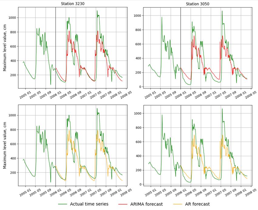
Water 2021, 13, 3482                                                                                                 10 of 28

                       it was decided to fill the gaps based on the available preceding and succeeding parts of
                       the time series. Also, there are ‘native’ gaps in the indicators related to ice conditions and
                       snow cover—for the warm season it was not filled for obvious reasons.
                             For this research, two methods of gap-filling were used depending on the size of
                       the gap. There were two general types of data: with pronounced seasonal component
                       and possessing some stationarity. While the size of the gap is small and calculations
                       are in values of up to ten or the time series especialty is stationarity, the autoregressive
                       algorithm was used. It provides less evaluation time and sufficient quality in such cases.
                       But for lengthy gaps and for time series with seasonality this approach as any other linear
                       approaches lead to inadequate results due to its specificity. This case is quite common in
                       the analyzed data of river monitoring-for some time series gaps reached several years.
                             For solving this problem, the following method was used. First of all, time series
                       with gaps was decomposed into three components: trend, seasonality, and residuals.
                       Decomposition was provided by the LOESS (locally estimated scatterplot smoothing)
                       method, which is common to use with natural data [61,62].
                             The several years of recordings were lost in data, but all time-series include thirty
                       years of observations, seasonal and trend components, which is the most significant to keep.
                       The combination of trend, seasonality and median value of the data in the range of the
                       gap fills it preserving the general peculiarities of time series. The results of the approach
                       described above are presented in Figure 5.

                       Figure 5. Filling in the gaps by extracting the seasonal component. (1) seasonal component of
                       time-series; (2) reconstructed time-series. The red boxes show the reconstructed sections of the time
                       series.

                       2.4. Time Series Forecasting
                             Currently, an approach based on the analysis of signals produced by the system is
                       widely used to study the properties of complex systems, including in experimental studies.
                       This is very relevant in cases where it is almost impossible to mathematically describe the
                       process under study, but we have some characteristic observable values at our disposal.
                       Therefore, the analysis of systems, especially in experimental studies, is often implemented
                       by processing the recorded signals—time series. For example, in meteorology—time series
                       from meteorological observations, etc.
                             It should be noted that the time series differs significantly from tabular data since its
                       analysis takes into account not only the statistical characteristics of the sample [63], but
                       also the temporal relationship. There are two main directions for the time series analysis:
                       statistical (probabilistic models, autoregressive models) and machine learning approaches.
                             Autoregressive models with a moving average (ARIMA) are used for statistical pro-
                       cessing of the time series. When using such models, it is necessary to bring the initial series
                       to a stationary form, which can be done using operations of trend removal application of
                       statistical estimates and noise filtering.
                             The set of models and methods that should be developed to apply ML to real data
                       should be selected according to the properties of the data and the modeling task. Auto-
                       mated machine learning (AutoML) technologies can be used to simplify the design process
Water 2021, 13, 3482 11 of 28
of such models. The automatic creation of ensemble models can improve the quality of
modeling of multiscale processes. The specifics of these data require a specific approach to
their processing.
This section discusses the application of composite pipelines obtained using automatic
machine learning algorithms to better predict multiscale processes represented by sensor
data. The proposed approach is based on the decomposition of the data stream and
correction of the modeling error achieved due to the specific structure of the composite
pipeline. However, simply adding or mixing multiple models may not be enough to handle
real data sets.
We can analyze a model created using the AutoML is details as shown in Figure 6. It
can be divided into two sub-pipelines: “smoothing-ridge-ridge regression” and “ridge-
ridge regression”, which are combined using the “ridge regression” node. The nodes of the
algorithm contain various operations. Using the described approach, the pipeline can be
configured in the following way: one of the models analyzes the periodic component, and
the other analyzes the components associated with trends.
Figure 6. Example of generated pipeline with operation names in the nodes.
• The smoothing operation is a Gaussian filter. Mathematically, the Gaussian filter mod-
ifies the input signal by convolution with the Gaussian function; this transformation
is also known as the Weierstrass transform. It is considered an ideal filter in the time
domain.
• The lagged operation is a comparison of a time series with a sequence of multidi-
mensional lagged vectors. An integer L (window length) is selected such that. These
vectors form the trajectory matrix of the original time series. This type of matrix is
known as the Hankel matrix elements of the anti-diagonals (that is, the diagonals
going from bottom to left to right) are equal.
• Ridge regression is a variation of linear regression, specially adapted for data that
demonstrate strong multicollinearity (that is, a strong correlation of features with each
other). The consequence of this is the instability of estimates of regression coefficients.
Estimates, for example, may have incorrect signs or values that far exceed those that
are acceptable for physical or practical reasons.
The pipeline “lagged-ridge regression” transforms the maximum daily water level
one-dimensional time-series into a trajectory matrix using a one-parameter shift procedure.
This makes it possible to use lagged vectors as features for a machine learning model
without involving exogenous data. Furthermore, ridge regression is applied to the obtained
trajectory matrix, since it is more likely that some columns of the matrix are correlated with
each other. It can lead to unstable estimates of regression coefficients. Adding a filtering
operation allows “smoothing out” the original time series, reducing the variance and
increasing the conditionality of the trajectory matrix at the stage of lagged transformation.
Visualization of the composite pipeline and operations in the nodes of this model is shown
in the Figure 7.Water 2021, 13, 3482 12 of 28
Filtred time- Trajectory Ridge Time-series
series matrix regression forecast
β2
Time-series OLS
data
estimate
Ridge
estimate
β1
β2 β2
OLS OLS
estimate estimate
Ridge Ridge
estimate estimate
β1 β1
Trajectory Ridge Ridge
matrix regression regression
Figure 7. The detailed representation of the composite pipeline structure and operations in the nodes.
The approaches described above were implemented in the AutoML framework FE-
DOT. This allowed us to quickly identify models when forecasting time series. Based on
this, we can say that the composite pipeline obtained using AutoML contains an interpre-
tation of physical processes described by a time series, since lagged vectors are used as
features that reflect the cyclicity and variability of processes. And at the same time, this
model takes into account the features of the data from the point of view of machine learning.
2.5. Multi-Output Regression
Also, we implemented a multi-regression model as an additional block of the com-
posite pipeline. We used the data historical data from weather stations and level gauges
(Table 2) to find the dependence between the target variables and the features.
Figure 8 presents the dynamics of the daily water level and the snow height simulta-
neously. The peaks of the orange curve can be interpreted as periods of snow accumulation
and extremes below zero can be called periods of snow melting. When the snow reaches a
minimum, the water level begins to rise.
Figure 8. The dependence of the amount of water on the snow height.
The target variable is a water level that depends on the features. In our case, it is
important to use not only the values at a current time of these features but also to take into
account the values over a period of time.
As an example, the correlation between the target variable and snow height can be
analyzed. To take into account whether the amount of snow decreased or increased over
the past few days, data aggregation can be used. We use several aggregation functions:
average, amplitude, most frequent, and summation value. The features in Table 3 areWater 2021, 13, 3482 13 of 28
calculated as an aggregation state for the past seven days, and the columns (“1”, “2” etc.)
are water level predictions for the seven days ahead.
It can be useful to take a closer look at the example with the amplitude of snow cover
height. We want to calculate the amount of melted snow over the past few days, as it
strongly correlates with the water level. In the case of snow height, this is not exactly the
amplitude, where the value is calculated by the formula max–min. For snow height, we
count the amount of melted precipitation over a certain time. The considered example
covers the period from 10 April 2020, to 30 April 2020, and the time interval for aggregation
is equal to seven days. In this case, we can find the difference between the current and past
day observations and accumulate difference if it is less than zero and continue accumulating
for the aggregating interval. So we can know “how many cm of snow melted during the
seven days”.
Table 3. Example of aggregated data for forecasting of seven days ahead.
w.amp w.mean s.mean s.amp Event 1 2 3 4 5 6 7
20 33.8 18.0 39.5 0 43 44 49 62 74 102 169
20 37.6 16.0 39.0 1 44 49 62 74 102 169 276
20 40.4 14.2 40.5 2 49 62 74 102 169 276 330
25 43.0 12.4 41.0 3 62 74 102 169 276 330 456
32 47.8 10.6 41.5 3 74 102 169 276 330 456 464
Figure 9 can be used to explain the process of features aggregation. The red line shows
the actual values of the snow height and the green line shows the aggregation state of the
accumulated melted snow over the past seven days. Let’s pay attention to the time period
indicated by the orange line, when the actual amount of snow decreases, the amount of
melted snow increases, which well describes the water level. In this case, accumulated
value allows estimating the amount of snow that has melted over a period of time and
using it as a feature for prediction.
Figure 9. The amount and aggregated state of snow from 10 April 2020 to 30 April 2020. Green is the
real amount of snow, red is aggregated state for past 7 days.
We have made similar transformations for other meteorological parameters. However,
there is a categorical feature describing the events on the river, and they are recorded in
the form of phrases including “Ice drifts”, “Excitement”, “Incomplete freeze-up”, “Jam
above the station”, etc. We decided to rank the events (Table 4) according to the degree
of influence on the water level in the river and have already applied aggregation-sum to
the ranked estimates. If the sum of the ranks is large, then we should expect a noticeable
change in the water level in the river and vice versa.Water 2021, 13, 3482 14 of 28
Table 4. Some events and importance ranks for them.
Event Importance Rank
The river has dried up 0
Distortion of water level and water flow by artificial phenomena 2
Blockage below the station 3
The set of additional features were obtained during the process of data preprocessing
and aggregation. Regular features are:
• temp (FLOAT)—average daily water temperature.
• ice-thickness (INT)—thickness of ice.
• snow-height (INT)—the height of snow on ice.
• discharge (FLOAT)—average daily water consumption, m3 /s.
• water-level (INT)—is the target variable indicating the maximum water level.
Aggregated features are:
• events—(TEXT)—the sum of events ranked by the degree for 30 days, correlated to
the water level.
• discharge-mean (FLOAT)—average for five days water consumption, m3 /s.
• temp-min (FLOAT)—minimum temperature on water level for 7 days. At low tem-
peratures, ice formation, slowing of the river flow and, as a result, an increase in the
water level is possible.
• ice-thickness-amplitude (INT)—amplitude thickness of ice for seven days shows an
increase or decrease in the thickness of the ice.
• snow-height-amplitude (INT)—amplitude of snow height. Directly proportional to
the water level.
• water-level-amplitude (INT)—the prediction of the water level depends heavily on
the data for the past few days. By aggregating the values for the past seven days, we
are essentially trying to predict a time series.
The prepared set of features allow us to build a multi-target regression model to
predict the water level for several days ahead. We decided to use the AutoML-based
approach to generate the multi-target regression pipelines that consist of models and data
operations. The best-found pipelines, based on validation data for flood forecasting, are
presented in Figure 10.
Figure 10. Several modelling pipelines generated by AutoML-based approach and used for the flood
forecasting.Water 2021, 13, 3482 15 of 28
The presented pipeline consists of two types of nodes: primary (blue) and secondary
(green); raw data is received in primary nodes. Each node is a model or an operation on
data. In the upper left corner, there is a pipeline, where the primary node is the principal
component analysis block. It is an operation on data that reduces the feature space while
not losing useful information for prediction. The secondary node in the pipeline is a
random forest regression, which is a model to give a final prediction. The combining
models and operations make it possible to build the sub-optimal pipeline that is effective in
terms of the predictive accuracy for the water level for seven days ahead. The identification
and optimization of the structure were conducted using the composite AutoML approach
described above.
2.6. Physical Modelling
In addition to the presented data-driven approaches, we chose to include a physics-
based element into the ensemble. As the base for our model we have utilized SRM
(Snowmelt-Runoff Model) [33], which is designed to calculate water discharge for the
mountainous river basins, where water, incoming into the river, originates from melting
snow and rain. The following assumption is stated: all discharge is generated by sources
inside the processed basin. It is limiting the model scope to the minor rivers. However,
in the analyzed case, the Lena river has a large water catchment area, that has varying
conditions and additional gauges located upstream which can be used for discharge
evaluations. We tried to alleviate the scope restriction by introducing a transfer term, that
connects the discharge in the downstream gauge with the discharge of the upstream one in
the previous day.
The main input variables, used in the SRM model, include temperature, from which
the number of degree-days Tn (◦ C · d) is calculated, snow cover Sn (%), and rainfall Rn (cm).
To initialize the modeling, a number of basin parameters shall be determined: snowmelt
and rain runoff coefficients (α1 and α3 correspondingly, dimensionless parameters), degree-
day factor (cm·◦ C−1 · d−1 ), and area A (km2 ). Additionally, we have to compute the
recession coefficient α4 = QQk , and α5 defining the transfer of the river water between
k −1
gauges (dimensionless), where k and k − 1 have to be evaluated during the periods with
no additional water intake into the river. The final equation for the discharge calculation
took form (1), where we make the prediction for the m-th gauge at n-th time point.
10000 m −1
Qm
n+1 = [ α1 α2 ( Tn + ∆Tn ) Sn + α3 Rn ] A (1 − α4 ) + α4 Q m m
n + α5 ( Q n − Q n ) (1)
86400
To calibrate the model we have utilized the differential evolution algorithm, that
searched for the model parameters, that produce the minimal error between model predic-
tions and observed values on the historical observations. The optimized function took form
of discrepancy between prediction Qm n pred , calculated by the Equation (1), and observed
m
value Qn obs , that has to be optimized in response to the parameter vector α = (α1 , ... , α5 ).
The specifics of the problem have introduced a number of constraints, caused by reasonable
boundaries of parameters.
| Qm m
n pred − Qn obs | −→ min (2)
α
The calibration was performed in two stages. At first, the data from the processed
period was split into two datasets by the presence of water input from the catchment. The
following assumption was stated: in periods with no snow cover and no rainfall, the river
discharge is determined only by the recession coefficient and the transfer. The stage of the
calibration was performed on this partial data for the reduced Equation (3). On the data,
that describes periods of water intake from the part of catchment, corresponding to the
studied gauge, the search of the remaining parameters was initialized.Water 2021, 13, 3482 16 of 28
m −1
Qm m m
n +1 = α 4 Q n + α 5 ( Q n − Q n ) (3)
Due to the simplicity of the proposed model, it can be relatively easy to interpret the
forecasts. By evaluating the terms of the Equation (1), model’s users can analyze which
factor between rainfall or snow melt contributes to the alteration of river discharge in the
particular moment. The variation of the river discharge, caused by these factors, can be
fully interpreted.
The final stage of the SRM-based approach is the transition from river discharge to the
water levels. To discover the dependency between these variables, the decision tree model
has been trained with the date and the discharge as the independent variables and the
maximum daily water level as the dependent one. Generally, the dependency is one-to-one
correspondence with the exception of cases, when the river flow is blocked by ice jams.
The input variables, used in the simulation are taken from the field observations and
from satellite data. Temperature and precipitation are measured at the meteorological
stations and then interpolated to the hydrological gauge in the manner, described in the
Section 2.3.
To assess the amount of snow cover, it was decided not to be limited only to mea-
surement data due to imperfect equipment, as well as the low quality of the results of
values interpolation from a point to an area. Therefore for calculating snow cover fraction,
remote sensing data from MODIS MOD10A1 product [64] was used. It provides spatial
data, which is more qualitative and complete than information from the meteorological
station (Figure 11).
Figure 11. NDSI spatial field obtained from the MODIS sensor for 28 February 2010. Base map source:
Bing Satellite. The date of capture for the base map is different.
Accumulation of runoff in each section of the watercourse due to melting of snow cover
occurs from a certain territory due to the relief. Extracting watershed by expert manual
solution is a laborious process, therefore the segmentation of territory on catchments
for each watercourse tributary was implemented with a capacity of GRASS geographic
information system (GIS). The algorithm r.watershed works on digital elevation model
(DEM) as input data, during processing, calculates water streams and returns the labels for
each catchment. Its core is an AT least-cost search algorithm [65] designed to minimize theWater 2021, 13, 3482 17 of 28
impact of DEM data errors. In this work open-source DEM - Shuttle Radar Topography
Mission (SRTM) [66] was used. Steps of calculating the watersheds for two hydro gauges
are presented in Figure 12.
Figure 12. Steps of watershed segmentation. (1) streamlines, generated on relief model; (2) catchment
segmentation for each tributary; (3) watershed segmentation for hydro gauges 3036 and 4045.
The Normalized-Difference Snow Index (NDSI), that was obtained from the MODIS
remote sensing and used for evaluation of the snow covered areas in the catchment, has
reliability issues, when applied to the evergreen coniferous forests, that are common in
the Eastern Siberia [67]. Additionally, the remote sensing data had to be filtered from the
measurements, taken in the conditions, when the view from the satellite is obstructed: over
the clouds, in nights, etc.
2.7. Quality Metrics for Forecasts
The following metrics were used:
• NSE—Nash–Sutcliffe model efficiency coefficient. The metric changes from −∞ to 1.
The closer the metric is to one, the better;
• MAE—Mean Absolute Error. The metric changes from 0 to ∞. The closer the metric
is to zero, the better. The units of this metric are the same as the target variable—
centimeters;
• SMAPE—Symmetric Mean Absolute Percentage Error. Varies from 0 to ∞. The closer
the metric is to zero, the better. Measured as a percentage.
The equations for NSE (Equation (4)), MAE (Equation (5)) and SMAPE (Equation (6))
are provided below. The following notation is used: n = number of elements in the sample,
yi is the prediction, xi the true value and x is averaged observed water level.Water 2021, 13, 3482 18 of 28
∑in=1 ( xi − yi )2
NSE = 1 − (4)
∑in=1 ( xi − x )2
∑in=1 |yi − xi |
MAE = (5)
n
100% n | yi − xi |
n i∑
SMAPE = (6)
=1
(| x i | + | yi |) /2
The specific approach was used to validate the algorithm using the metrics described
above. The composite pipeline is able to provide forecast yn for n days ahead with the
following time steps for forecast {t + 1, ..., t + n}. In this case, the retrospective data X is
used to train the models in the pipeline. To prepare a forecast for the interval from t + 1 to
t + n the m values of the predictor Xm for time steps {t, ..., t − m} are required. Respectively,
the sub-sample of retrospective data {t + n, ..., t + n − m} is required to obtain the forecast
from t + n to t + 2 × n. The trained pipeline can predict the values for n next elements if
the set of predictors with the specified length is provided. So, the length of the validation
part of the time series can be arbitrary. In the paper, the length of the validation horizon
was equal to 805 elements (days).
The distribution of error across forecast horizons was also additionally investigated.
For this purpose Metrics were measured only on forecasts of 1, 2, 3, 4, 5 and 7 days in
advance. In addition to calculating metrics, an extensive analysis of graphical materials:
predictions and error plots are presented.
3. Results
3.1. Validation
Validation of the results was carried out by comparing the predicted water level values
and the actual values recorded at the hydro gauges. Below all models have been configured
to give a forecast for seven days ahead. Since preparing and tuning a composite pipeline
requires a multi-step approach, the following strategy was used. Models identification
(search for optimal structure and hyperparameters values) in an automated way was
performed on data for the period from 1985 to 2006. From 2006 to 2010, the ensemble model
was prepared and tuned. Finally, validation was performed with daily data collected from
2010 to 2012. These years were chosen for validation because this period was relatively
challenging spring floodwater on Lena River [51].
Hydro gauges with the following identifiers were used for validation: 3019, 3027, 3028,
3029, 3030, 3035, 3041, 3045, 3050, 3230—ten posts in total. The validation of individual
models and the ensemble is presented below.
Several examples of the forecasts obtained from a model based on time series are
shown in Figure 13. For prediction on each subsequent validation block, the actual values
of the series were used. It is possible to estimate the model quality for 115 validation blocks
of seven elements—a total of 805 elements for each post.
As can be seen from Figure 13, the proposed model can efficiently predict the level
rise during floods (e.g., beginning of summer when rapid raise of water level is observed).
The average value of the metrics confirms that the time series model is relatively accurate
even without including it in the ensemble: NSE—0.74.Water 2021, 13, 3482 19 of 28
Figure 13. Validation of time series forecasting model for several hydro gauges. Forecasting horizon—
seven days.
For the multi-target regression model, the forecast efficiency was also estimated:
NSE—0.72. “Actual vs. predicted” plots for comparison forecasts obtained from different
models provided in Figure 14.
As can be seen from Figure 14, there is no model that is significantly more accurate
than the others. The same is confirmed by the metric values. So, it was decided to use
ensemble to remove drawbacks from individual blocks predictions (Figure 15).
As can be seen from the figure, the most accurate forecast is given by the ensemble of
models. Also, validation was performed not only on the entire validation period but only
on the parts when the extreme water level rises occur (April–July). This period is referred
to below as “Spring/Summer”. Results of validation composite pipeline and individual
blocks are shown in Table 5.
Additionally, experiments were conducted to determine how different the values of
the metrics on the training (Train), the test (Test) and the validation sample (Validation).
The results for all model blocks for station 3045 are shown in Table 6.
To better appreciate the robustness of the forecast, the distribution of error across
forecast horizons was investigated. For that purpose, the following forecast horizons (days)
were tested: 1, 2, 3, 4, 5, 6, 7 (Figure 16).Water 2021, 13, 3482 20 of 28
Figure 14. Actual values vs. predicted for the two hydro gauges. Time series and multi-target models
forecasts are shown for validation part. Forecast horizon is seven days.
Figure 15. Forecasts of individual blocks and ensemble on the validation part. The most relevant
parts of time series are shown in the sub-figures. Forecast horizon is seven days.Water 2021, 13, 3482 21 of 28
Table 5. Validation metrics for ensemble and individual machine learning models obtained for ten
hydro gauges.
All Period Spring/Summer
Metric Time Multi Time Multi
Ensemble Ensemble
Series Target Series Target
NSE 0.74 0.72 0.80 0.60 0.61 0.71
MAE, cm 45.02 54.84 45.51 80.78 91.86 78.92
SMAPE, % 28.44 31.97 28.65 28.80 31.86 28.97
Table 6. The value of the NSE and MAE metrics for stand-alone models and for ensemble.
NSE MAE, cm
Model
Train Test Validation Train Test Validation
Time series 0.92 0.90 0.83 33.1 37.1 43.9
Multi-target 0.94 0.89 0.74 20.1 40.6 54.6
SRM 0.90 0.74 0.74 72.1 81.2 93.5
Ensemble 0.94 0.92 0.84 28.8 28.9 41.8
Figure 16. Error metrics (NSE and SMAPE) of ensemble model for several forecasting horizons.
As can be seen from the Figure 16, as the forecast horizon increases, the NSE value falls
the most. At the same time, the MAE metric increases slightly. In can be concluded that
the predictive efficiency of the model decreases in the domain of level variance prediction
when the forecast horizon increases.
Finally, experiments with different gap sizes in training sample were conducted to
find out how robust the model is to the presence of gaps. For example, the water level
data without gaps were prepared for station 3045. In these series, the gaps were generated
and reconstructed using the methods described in the current paper. Then, the ensemble
trained on recovered data. The results of error estimation presented in Table 7.
Table 7. Dependence of the forecast error on the gap size in the training sample for ensemble model.
Metrics are shown for test part.
Gaps Size (%) 0 10 20 30 40
NSE 0.92 0.92 0.89 0.80 0.81
MAE, cm 28.9 28.9 31.4 35.9 41.1
SMAPE, % 25.4 26.2 29.9 33.5 39.2Water 2021, 13, 3482 22 of 28
It is clear from the table, that as the size of the gaps increases, the ensemble error on
the test sample increases. However, this increase can be considered acceptable. Note that
successful identification of machine learning models usually requires a lot of data.
3.2. Comparison
The composite pipeline obtained with the AutoML-based approach can be quite com-
plex. Therefore, for a more objective assessment, we compared the quality of forecasting
results with the most common autoregressive models and physical-based model.
It should be noted that the seasonal component clearly exists in the data. For there
reason, using only autoregression methods can not bring a quality result inherently. So
seasonal and trend decomposition described above was used to separate seasonal com-
ponents predetermined by frequency estimation period. Two models were used for the
prediction of series without seasonality: AR and ARIMA. After the evaluation, the seasonal
component was returned to prediction.
Water level prediction and time-series analysis via ARIMA is common practice [39,68].
AR is more often found as part of ensembles [38], due to its naivety to use separately. The
hyperparameters for the models were chosen according to the lowest value of the Akaike
criterion (AIC) on the training sample. So, a prediction for the validation sample was made
for each station with the calculation of the previously described metrics. Examples of the
forecast by two models are presented in Figure 17. The average values of metrics for AR:
NSE—0.59, ARIMA: NSE—0.56.
Figure 17. Forecast of statistical models (AR and ARIMA) on the validation part of water level time
series.
The results of validation for all models are summarized in a common Table 8 for
comparison.You can also read