TROPOMI ATBD of the Aerosol Layer Height - Sentinel Online
←
→
Page content transcription
If your browser does not render page correctly, please read the page content below
TROPOMI ATBD of the Aerosol
Layer Height

document number : S5P-KNMI-L2-0006-RP
authors             : M. de Graaf, J.F. de Haan and A.F.J. Sanders
CI identification   : CI-7430-ATBD_Aerosol_Layer_Height
issue               : 2.2.0
date                : 2021-07-05
status              : Released
TROPOMI ATBD Aerosol Layer Height                          S5P-KNMI-L2-0006-RP
issue 2.2.0, 2021-07-05 – Released                                 Page 2 of 75

Document approval record
                 digital signature

                                 Digitally signed by Martin de Graaf
                 Martin de Graaf Date: 2021.07.02 12:23:50 +02'00'
 Prepared:

 Checked:

 Approved PM:

 Approved PI: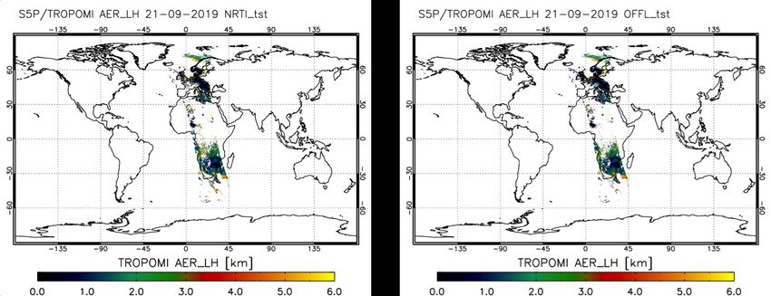
TROPOMI ATBD Aerosol Layer Height                                                      S5P-KNMI-L2-0006-RP
issue 2.2.0, 2021-07-05 – Released                                                             Page 3 of 75

Document change record

 issue    date         item          comments
 0.0.1    2012-09-10   All           Initial version.
 0.0.2    2012-09-25   All           Updated with feed from KNMI Level-2 team.
 0.1.0    2012-09-27   -             Released for first review by Level-2 Working Group.
 0.1.1    2012-11-16   All           Updated with feedback from aerosol science verification team.
                                     Document number changed from S5P-KNMI-L2-0115-RP to S5P-
                                     KNMI-L2-0006-RP.
 0.2.0    2012-11-16   -             Released for first review by ESA.
                                     Section Absorbing Aerosol Index moved to separate ATBD
                                     (S5P-KNMI-L2-0008-RP).
 0.2.1    2013-06-04   All
                                     Added error analysis.
                                     Completed and revised other sections.
 0.3.0    2013-06-04   -             Released for Level-2 Working Group.
                       All           Updated with feedback from aerosol science verification team
 0.3.1    2013-06-21                 (no major changes).
                       10            Added application to GOSAT spectra (Section 10).
 0.5.0    2013-06-21   -             Released for external science review.
                                     Updated with feedback from external science reviewers.
                       6.4.1         Clarified text on ignoring polarization in Section 6.4.1.
 0.5.1    2013-11-29
                       9.9           Added paragraph on fluorescence to Section 8.9.
                                     Minor other clarifications throughout the text.
 0.9.0    2013-11-29   -             Released for external science review.
                       4             Section Instrument (Section 4) moved to separate ATBD
                                     (S5P-KNMI-L2-0010-RP).
 0.9.1    2014-04-15   10            Revised and completed Section 10; section renamed to
                                     Application to GOME-2 spectra.
                       4.7,11        Updated Section 4.7 and Section 11.
 0.10.0   2014-04-15   -             Released for Critical Design Review.
                       7             Revised Section 7
 0.10.1   2014-09-30   5.3.3         Added paragraph to Section 5.3.3.
                                     Several minor clarifications throughout the text.
 0.11.0   2014-09-30   -             Released for review by ESA.
                       7             Updated pixel selection with description of VIIRS cloud mask.
 0.11.1   2015-09-04   6.2,7.3.3     Added remark on alternative surface albedo climatologies.
                                     Several minor changes throughout the text.
 0.13.0   2015-09-04   -             Limited release to S5P Validation Team.
                       4.2,4.5-6,    Updated sections on algorithm heritage, algorithm overview,
                       5.3,5.5,      development risks, the atmospheric model, the instrument model
                       6.2           and the state vector composition. Main changes: surface albedo
                                     removed from state vector, reduction of fit window to 758–762 nm,
 0.13.1   2016-01-29                 interpretation of Aerosol Layer Height parameter, other
                                     conclusions from recent GOME-2 and SCIAMACHY case studies
                                     included in the ATBD.
                       11            Updated conclusion and outlook.
                                     Several minor changes throughout the text.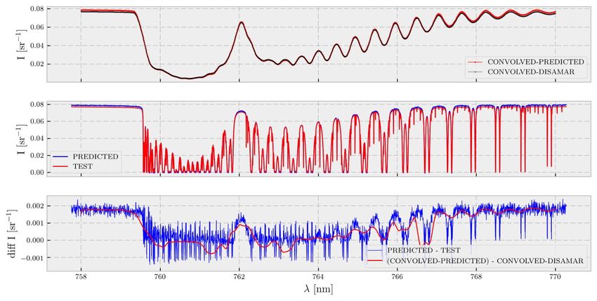
TROPOMI ATBD Aerosol Layer Height                                                   S5P-KNMI-L2-0006-RP
issue 2.2.0, 2021-07-05 – Released                                                          Page 4 of 75

 issue   date         item           comments
 1.0.0   2016-01-29   -              Public release.
 1.0.1   2019-06-24   5              Update forward model with neural network estimate of O2-A band
                                     reflectances. First validation and verifcation.
 1.1.0   2019-09-30   -              Public release.
                                     Update of VIIRS CF definition
                      5.1.1
                                     Redefined pixel selection criteria.
 1.1.1   2020-12-11   5.1.5
                                     Update of timeliness including VCM
                      7.3
                                     Several minor clarifications throughout the text.
                      4              Minor updates
 2.0.0   2020-06-24
                      9              Removed obsolete
 2.2.0   2021-07-05   -              Public release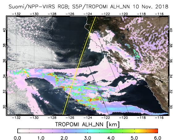
TROPOMI ATBD Aerosol Layer Height                                                                                                                                                S5P-KNMI-L2-0006-RP
issue 2.2.0, 2021-07-05 – Released                                                                                                                                                       Page 5 of 75

Contents
Document approval record . . . . . . . . . . . . . . . . . . . . . . . . . . . . . . . . . . . . . . . . . . . . . . . . . . . . . . . . . . . . . . . . . . . . . . . . . . . . . . . .                              2
Document change record . . . . . . . . . . . . . . . . . . . . . . . . . . . . . . . . . . . . . . . . . . . . . . . . . . . . . . . . . . . . . . . . . . . . . . . . . . . . . . . . . .                            3
List of Tables . . . . . . . . . . . . . . . . . . . . . . . . . . . . . . . . . . . . . . . . . . . . . . . . . . . . . . . . . . . . . . . . . . . . . . . . . . . . . . . . . . . . . . . . . . . . . . . .        6
List of Figures . . . . . . . . . . . . . . . . . . . . . . . . . . . . . . . . . . . . . . . . . . . . . . . . . . . . . . . . . . . . . . . . . . . . . . . . . . . . . . . . . . . . . . . . . . . . . . .          7
1                   Introduction . . . . . . . . . . . . . . . . . . . . . . . . . . . . . . . . . . . . . . . . . . . . . . . . . . . . . . . . . . . . . . . . . . . . . . . . . . . . . . . . . . . . . .          11
1.1                 Identification . . . . . . . . . . . . . . . . . . . . . . . . . . . . . . . . . . . . . . . . . . . . . . . . . . . . . . . . . . . . . . . . . . . . . . . . . . . . . . . . . . . . . . .      11
1.2                 Purpose and objective . . . . . . . . . . . . . . . . . . . . . . . . . . . . . . . . . . . . . . . . . . . . . . . . . . . . . . . . . . . . . . . . . . . . . . . . . . . .                     11
1.3                 Document overview . . . . . . . . . . . . . . . . . . . . . . . . . . . . . . . . . . . . . . . . . . . . . . . . . . . . . . . . . . . . . . . . . . . . . . . . . . . . . . .                   11
1.4                 Acknowledgements . . . . . . . . . . . . . . . . . . . . . . . . . . . . . . . . . . . . . . . . . . . . . . . . . . . . . . . . . . . . . . . . . . . . . . . . . . . . . . .                    11
2                   Applicable and reference documents . . . . . . . . . . . . . . . . . . . . . . . . . . . . . . . . . . . . . . . . . . . . . . . . . . . . . . . . .                                              12
2.1                 Applicable documents . . . . . . . . . . . . . . . . . . . . . . . . . . . . . . . . . . . . . . . . . . . . . . . . . . . . . . . . . . . . . . . . . . . . . . . . . . . .                      12
2.2                 Reference documents . . . . . . . . . . . . . . . . . . . . . . . . . . . . . . . . . . . . . . . . . . . . . . . . . . . . . . . . . . . . . . . . . . . . . . . . . . . .                       12
2.3                 Electronic references . . . . . . . . . . . . . . . . . . . . . . . . . . . . . . . . . . . . . . . . . . . . . . . . . . . . . . . . . . . . . . . . . . . . . . . . . . . . .                   13
3                   Terms, definitions and abbreviated terms . . . . . . . . . . . . . . . . . . . . . . . . . . . . . . . . . . . . . . . . . . . . . . . . . . . .                                                  14
3.1                 Terms and definitions . . . . . . . . . . . . . . . . . . . . . . . . . . . . . . . . . . . . . . . . . . . . . . . . . . . . . . . . . . . . . . . . . . . . . . . . . . . . .                   14
3.2                 Acronyms and Abbreviations . . . . . . . . . . . . . . . . . . . . . . . . . . . . . . . . . . . . . . . . . . . . . . . . . . . . . . . . . . . . . . . . . . . . .                              14
3.3                 Symbols . . . . . . . . . . . . . . . . . . . . . . . . . . . . . . . . . . . . . . . . . . . . . . . . . . . . . . . . . . . . . . . . . . . . . . . . . . . . . . . . . . . . . . . . . . .     16
4                   Introduction to Aerosol Layer Height product . . . . . . . . . . . . . . . . . . . . . . . . . . . . . . . . . . . . . . . . . . . . . . .                                                        18
4.1                 Product description . . . . . . . . . . . . . . . . . . . . . . . . . . . . . . . . . . . . . . . . . . . . . . . . . . . . . . . . . . . . . . . . . . . . . . . . . . . . . . .                 18
4.2                 Heritage. . . . . . . . . . . . . . . . . . . . . . . . . . . . . . . . . . . . . . . . . . . . . . . . . . . . . . . . . . . . . . . . . . . . . . . . . . . . . . . . . . . . . . . . . . . .   19
4.3                 Product requirements . . . . . . . . . . . . . . . . . . . . . . . . . . . . . . . . . . . . . . . . . . . . . . . . . . . . . . . . . . . . . . . . . . . . . . . . . . . . .                    20
4.4                 Overview of the retrieval algorithm . . . . . . . . . . . . . . . . . . . . . . . . . . . . . . . . . . . . . . . . . . . . . . . . . . . . . . . . . . . . . . .                                 20
4.5                 Updates . . . . . . . . . . . . . . . . . . . . . . . . . . . . . . . . . . . . . . . . . . . . . . . . . . . . . . . . . . . . . . . . . . . . . . . . . . . . . . . . . . . . . . . . . . . .   22
4.6                 Developments . . . . . . . . . . . . . . . . . . . . . . . . . . . . . . . . . . . . . . . . . . . . . . . . . . . . . . . . . . . . . . . . . . . . . . . . . . . . . . . . . . . . .            23
4.7                 Terminology . . . . . . . . . . . . . . . . . . . . . . . . . . . . . . . . . . . . . . . . . . . . . . . . . . . . . . . . . . . . . . . . . . . . . . . . . . . . . . . . . . . . . . .         23
5                   Algorithm description . . . . . . . . . . . . . . . . . . . . . . . . . . . . . . . . . . . . . . . . . . . . . . . . . . . . . . . . . . . . . . . . . . . . . . . . . . .                       25
5.1                 Spatial data selection . . . . . . . . . . . . . . . . . . . . . . . . . . . . . . . . . . . . . . . . . . . . . . . . . . . . . . . . . . . . . . . . . . . . . . . . . . . . .                  25
5.1.1               Cloud mask . . . . . . . . . . . . . . . . . . . . . . . . . . . . . . . . . . . . . . . . . . . . . . . . . . . . . . . . . . . . . . . . . . . . . . . . . . . . . . . . . . . . . . . .        25
5.1.2               Snow or ice covered pixels . . . . . . . . . . . . . . . . . . . . . . . . . . . . . . . . . . . . . . . . . . . . . . . . . . . . . . . . . . . . . . . . . . . . . . .                          26
5.1.3               Sunglint . . . . . . . . . . . . . . . . . . . . . . . . . . . . . . . . . . . . . . . . . . . . . . . . . . . . . . . . . . . . . . . . . . . . . . . . . . . . . . . . . . . . . . . . . . .    26
5.1.4               Pixels containing aerosol . . . . . . . . . . . . . . . . . . . . . . . . . . . . . . . . . . . . . . . . . . . . . . . . . . . . . . . . . . . . . . . . . . . . . . . . .                       26
5.1.5               Pixel selection scheme . . . . . . . . . . . . . . . . . . . . . . . . . . . . . . . . . . . . . . . . . . . . . . . . . . . . . . . . . . . . . . . . . . . . . . . . . . .                      26
5.2                 Forward model . . . . . . . . . . . . . . . . . . . . . . . . . . . . . . . . . . . . . . . . . . . . . . . . . . . . . . . . . . . . . . . . . . . . . . . . . . . . . . . . . . . .             27
5.2.1               Overview . . . . . . . . . . . . . . . . . . . . . . . . . . . . . . . . . . . . . . . . . . . . . . . . . . . . . . . . . . . . . . . . . . . . . . . . . . . . . . . . . . . . . . . . . . .    27
5.2.2               Radiative transfer model . . . . . . . . . . . . . . . . . . . . . . . . . . . . . . . . . . . . . . . . . . . . . . . . . . . . . . . . . . . . . . . . . . . . . . . . . .                      28
5.2.3               The Neural Network forward model . . . . . . . . . . . . . . . . . . . . . . . . . . . . . . . . . . . . . . . . . . . . . . . . . . . . . . . . . . . . . .                                      28
5.2.4               NN configuration and training . . . . . . . . . . . . . . . . . . . . . . . . . . . . . . . . . . . . . . . . . . . . . . . . . . . . . . . . . . . . . . . . . . . .                             30
6                   Algorithm description: Retrieval method . . . . . . . . . . . . . . . . . . . . . . . . . . . . . . . . . . . . . . . . . . . . . . . . . . . . .                                                 34
6.1                 Optimal Estimation . . . . . . . . . . . . . . . . . . . . . . . . . . . . . . . . . . . . . . . . . . . . . . . . . . . . . . . . . . . . . . . . . . . . . . . . . . . . . . . .                34
6.2                 State vector elements and a priori information . . . . . . . . . . . . . . . . . . . . . . . . . . . . . . . . . . . . . . . . . . . . . . . . . .                                                35
6.2.1               Height variable . . . . . . . . . . . . . . . . . . . . . . . . . . . . . . . . . . . . . . . . . . . . . . . . . . . . . . . . . . . . . . . . . . . . . . . . . . . . . . . . . . . .           35
6.2.2               Profile parameterization . . . . . . . . . . . . . . . . . . . . . . . . . . . . . . . . . . . . . . . . . . . . . . . . . . . . . . . . . . . . . . . . . . . . . . . . . .                      36
6.3                 Convergence of retrieval and uniqueness of solution . . . . . . . . . . . . . . . . . . . . . . . . . . . . . . . . . . . . . . . . . . .                                                         36
7                   Feasibility . . . . . . . . . . . . . . . . . . . . . . . . . . . . . . . . . . . . . . . . . . . . . . . . . . . . . . . . . . . . . . . . . . . . . . . . . . . . . . . . . . . . . . . .       38
7.1                 Timeliness . . . . . . . . . . . . . . . . . . . . . . . . . . . . . . . . . . . . . . . . . . . . . . . . . . . . . . . . . . . . . . . . . . . . . . . . . . . . . . . . . . . . . . . . .      38
7.2                 VIIRS cloud mask . . . . . . . . . . . . . . . . . . . . . . . . . . . . . . . . . . . . . . . . . . . . . . . . . . . . . . . . . . . . . . . . . . . . . . . . . . . . . . . . .                39
7.3                 Input data for the Aerosol Layer Height algorithm . . . . . . . . . . . . . . . . . . . . . . . . . . . . . . . . . . . . . . . . . . . . . . .                                                   41
7.3.1               TROPOMI Level-1b . . . . . . . . . . . . . . . . . . . . . . . . . . . . . . . . . . . . . . . . . . . . . . . . . . . . . . . . . . . . . . . . . . . . . . . . . . . . . . .                    41
7.3.2               Dynamic input . . . . . . . . . . . . . . . . . . . . . . . . . . . . . . . . . . . . . . . . . . . . . . . . . . . . . . . . . . . . . . . . . . . . . . . . . . . . . . . . . . . . .           41
7.3.3               Static input. . . . . . . . . . . . . . . . . . . . . . . . . . . . . . . . . . . . . . . . . . . . . . . . . . . . . . . . . . . . . . . . . . . . . . . . . . . . . . . . . . . . . . . . .     43
7.4                 Robustness against instrumental errors . . . . . . . . . . . . . . . . . . . . . . . . . . . . . . . . . . . . . . . . . . . . . . . . . . . . . . . . .                                          43
7.5                 Data product description . . . . . . . . . . . . . . . . . . . . . . . . . . . . . . . . . . . . . . . . . . . . . . . . . . . . . . . . . . . . . . . . . . . . . . . . . .                      44
TROPOMI ATBD Aerosol Layer Height                                                                                                                                     S5P-KNMI-L2-0006-RP
issue 2.2.0, 2021-07-05 – Released                                                                                                                                            Page 6 of 75

8        Error analysis . . . . . . . . . . . . . . . . . . . . . . . . . . . . . . . . . . . . . . . . . . . . . . . . . . . . . . . . . . . . . . . . . . . . . . . . . . . . . . . . . . . .            45
8.1      Performance of the neural network forward model . . . . . . . . . . . . . . . . . . . . . . . . . . . . . . . . . . . . . . . . . . . . . .                                                       45
8.2      Default settings for the error analysis . . . . . . . . . . . . . . . . . . . . . . . . . . . . . . . . . . . . . . . . . . . . . . . . . . . . . . . . . . . .                                   46
8.3      Baseline precision of Aerosol Layer Height. . . . . . . . . . . . . . . . . . . . . . . . . . . . . . . . . . . . . . . . . . . . . . . . . . . . . .                                             47
8.4      Required knowledge of aerosol type . . . . . . . . . . . . . . . . . . . . . . . . . . . . . . . . . . . . . . . . . . . . . . . . . . . . . . . . . . . . .                                      51
8.4.1    Single scattering albedo . . . . . . . . . . . . . . . . . . . . . . . . . . . . . . . . . . . . . . . . . . . . . . . . . . . . . . . . . . . . . . . . . . . . . . . . . .                      51
8.4.2    Phase function . . . . . . . . . . . . . . . . . . . . . . . . . . . . . . . . . . . . . . . . . . . . . . . . . . . . . . . . . . . . . . . . . . . . . . . . . . . . . . . . . . . .            53
8.4.3    Conclusion. . . . . . . . . . . . . . . . . . . . . . . . . . . . . . . . . . . . . . . . . . . . . . . . . . . . . . . . . . . . . . . . . . . . . . . . . . . . . . . . . . . . . . . . .       55
8.5      Role of a priori knowledge of the surface albedo. . . . . . . . . . . . . . . . . . . . . . . . . . . . . . . . . . . . . . . . . . . . . . . .                                                   55
8.6      Fitting surface albedo to compensate errors in single scattering albedo . . . . . . . . . . . . . . . . . . . . . .                                                                               58
8.7      Effect of uncertainty in a priori meteorological data . . . . . . . . . . . . . . . . . . . . . . . . . . . . . . . . . . . . . . . . . . . . .                                                   60
8.7.1    Temperature profile . . . . . . . . . . . . . . . . . . . . . . . . . . . . . . . . . . . . . . . . . . . . . . . . . . . . . . . . . . . . . . . . . . . . . . . . . . . . . . .                 60
8.7.2    Surface pressure . . . . . . . . . . . . . . . . . . . . . . . . . . . . . . . . . . . . . . . . . . . . . . . . . . . . . . . . . . . . . . . . . . . . . . . . . . . . . . . . . .              61
8.7.3    Conclusion. . . . . . . . . . . . . . . . . . . . . . . . . . . . . . . . . . . . . . . . . . . . . . . . . . . . . . . . . . . . . . . . . . . . . . . . . . . . . . . . . . . . . . . . .       63
8.8      Aerosol pressure biases due to cloud contamination . . . . . . . . . . . . . . . . . . . . . . . . . . . . . . . . . . . . . . . . . . .                                                          63
8.9      Alternative profile parameterization: aerosol layer with variable pressure thickness. . . . . . . . . .                                                                                           64
8.10     Interference of chlorophyll fluorescence . . . . . . . . . . . . . . . . . . . . . . . . . . . . . . . . . . . . . . . . . . . . . . . . . . . . . . . . .                                        65
8.11     Instrumental errors . . . . . . . . . . . . . . . . . . . . . . . . . . . . . . . . . . . . . . . . . . . . . . . . . . . . . . . . . . . . . . . . . . . . . . . . . . . . . . . .               67
8.11.1   Stray light . . . . . . . . . . . . . . . . . . . . . . . . . . . . . . . . . . . . . . . . . . . . . . . . . . . . . . . . . . . . . . . . . . . . . . . . . . . . . . . . . . . . . . . . . .   67
8.11.2   Wavelength calibration . . . . . . . . . . . . . . . . . . . . . . . . . . . . . . . . . . . . . . . . . . . . . . . . . . . . . . . . . . . . . . . . . . . . . . . . . . . .                    67
9        Validation . . . . . . . . . . . . . . . . . . . . . . . . . . . . . . . . . . . . . . . . . . . . . . . . . . . . . . . . . . . . . . . . . . . . . . . . . . . . . . . . . . . . . . . . .      69
9.1      Validation with lidar measurements . . . . . . . . . . . . . . . . . . . . . . . . . . . . . . . . . . . . . . . . . . . . . . . . . . . . . . . . . . . . . .                                    69
9.1.1    First validation with Caliop . . . . . . . . . . . . . . . . . . . . . . . . . . . . . . . . . . . . . . . . . . . . . . . . . . . . . . . . . . . . . . . . . . . . . . . .                      69
9.2      Intercomparison of passive satellite retrievals . . . . . . . . . . . . . . . . . . . . . . . . . . . . . . . . . . . . . . . . . . . . . . . . . . .                                             69
9.3      Dedicated validation campaigns . . . . . . . . . . . . . . . . . . . . . . . . . . . . . . . . . . . . . . . . . . . . . . . . . . . . . . . . . . . . . . . . .                                  70
10       Conclusion and outlook . . . . . . . . . . . . . . . . . . . . . . . . . . . . . . . . . . . . . . . . . . . . . . . . . . . . . . . . . . . . . . . . . . . . . . . .                            71
11       References. . . . . . . . . . . . . . . . . . . . . . . . . . . . . . . . . . . . . . . . . . . . . . . . . . . . . . . . . . . . . . . . . . . . . . . . . . . . . . . . . . . . . . . .         72

List of Tables
1        Scene-dependent input model parameters for the NN model. . . . . . . . . . . . . . . . . . . . . . . . . . . . . . . . . .                                                                        29
2        State vector elements and typical a priori values and errors for the Aerosol Layer Height
         retrieval algorithm. In the current implementation, the state vector contains the parameters
         printed in bold. For an explanation, see text. . . . . . . . . . . . . . . . . . . . . . . . . . . . . . . . . . . . . . . . . . . . . . . . . . . . .                                            35
3        TROPOMI Level-1b input data.. . . . . . . . . . . . . . . . . . . . . . . . . . . . . . . . . . . . . . . . . . . . . . . . . . . . . . . . . . . . . . . . . . .                                 41
4        Dynamic input data for off-line processing and reprocessing. . . . . . . . . . . . . . . . . . . . . . . . . . . . . . . . . . .                                                                  42
5        Dynamic input data for near real-time processing. . . . . . . . . . . . . . . . . . . . . . . . . . . . . . . . . . . . . . . . . . . . . . .                                                     42
6        Static input data. . . . . . . . . . . . . . . . . . . . . . . . . . . . . . . . . . . . . . . . . . . . . . . . . . . . . . . . . . . . . . . . . . . . . . . . . . . . . . . . . . .            43
7        Level-2 output data. . . . . . . . . . . . . . . . . . . . . . . . . . . . . . . . . . . . . . . . . . . . . . . . . . . . . . . . . . . . . . . . . . . . . . . . . . . . . . . .                44
8        Surface types and corresponding albedos considered in the error analysis. . . . . . . . . . . . . . . . . . .                                                                                     47
9        Correlation coefficients between errors in fit parameters for an aerosol layer with optical
         thickness of 0.5 at 800 hPa over sea / ocean and vegetated land. The solar zenith angle
         is 60◦ and the viewing direction is nadir. The height variable is altitude (in km) instead of
         pressure (in hPa). . . . . . . . . . . . . . . . . . . . . . . . . . . . . . . . . . . . . . . . . . . . . . . . . . . . . . . . . . . . . . . . . . . . . . . . . . . . . . . . . .              50
10       True values, a priori values and a priori errors used in the retrieval simulations of Figure 17
         investigating the sensitivity of retrieval to the assumed single scattering albedo. . . . . . . . . . . . . .                                                                                     51
11       Optical properties at the O2 A band for the three aerosol models used in the retrieval
         simulations of Figure 21 (based on [12]). Properties for the Dust model are based on T-
         matrix calculations, which are kindly provided by Oleg Dubovik and co-workers; for the other
         two models we performed Mie calculations. . . . . . . . . . . . . . . . . . . . . . . . . . . . . . . . . . . . . . . . . . . . . . . . . . . . . .                                               53
12       True values, a priori values and a priori errors used in the retrieval simulations of Figure 21
         investigating the sensitivity of retrieval to the assumed phase function. . . . . . . . . . . . . . . . . . . . . . . .                                                                           54
13       A priori error in the surface albedo for the three types of retrieval investigating the effect of an
         error in climatological surface albedo values. . . . . . . . . . . . . . . . . . . . . . . . . . . . . . . . . . . . . . . . . . . . . . . . . . . .                                              57
14       True values, a priori values and a priori errors used in the retrieval simulations of Figure 23
         investigating the sensitivity of retrieval to the assumed phase function. . . . . . . . . . . . . . . . . . . . . . . .                                                                           58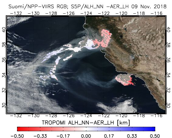
TROPOMI ATBD Aerosol Layer Height                                                                                                                                   S5P-KNMI-L2-0006-RP
issue 2.2.0, 2021-07-05 – Released                                                                                                                                          Page 7 of 75

15      Retrieved aerosol pressures for a number of atmospheric scenarios when an offset of 1 K is
        applied to the mid-latitude summer temperature profile in the simulation. . . . . . . . . . . . . . . . . . . . . .                                                                                61
16      Retrieved aerosol pressures for a number of atmospheric scenarios when the true surface
        pressure is 1011 hPa while the surface pressure assumed in retrieval is 1013 hPa. . . . . . . . . .                                                                                                62
17      True values, a priori values and a priori errors used in the retrieval simulations of Figure 19
        investigating the sensitivity of retrieval to the assumed single scattering albedo. . . . . . . . . . . . . .                                                                                      66
18      Pressure biases and retrieved optical thicknesses in case of additive offsets applied to the
        radiance and irradiance spectrum. The aerosol layer has an optical thickness of 0.5 and is at
        700 hPa over sea / ocean or vegetated land. Stray light offsets are constant with wavelength
        and they are defined as percentages of the (ir)radiance at 758 nm. . . . . . . . . . . . . . . . . . . . . . . . . . . .                                                                           67
19      Pressure biases and retrieved optical thicknesses in case the width of the radiance and
        irradiance slit functions in the simulation differs from the width of the slit functions assumed in
        the retrieval. The aerosol layer has an optical thickness of 0.5 and is at 700 hPa over sea /
        ocean or vegetated land. The FWHM of the radiance and irradiance slit functions in retrieval
        is 0.5 nm. . . . . . . . . . . . . . . . . . . . . . . . . . . . . . . . . . . . . . . . . . . . . . . . . . . . . . . . . . . . . . . . . . . . . . . . . . . . . . . . . . . . . . . . . . .     68

List of Figures
1       Simulated reflectance spectra of the O2 A band at a spectral resolution (FWHM) of 0.5 nm
        for a scene containing a representative aerosol layer. The aerosol layer is between 950 and
        850 hPa (green line) or between 540 and 475 hPa (blue line). The 1-σ measurement errors
        on reflectance are smaller than the width of the plotting lines: anticipated signal-to-noise
        ratios for these spectra (based on [56]) are about 645 in the continuum and 302 and 207
        in the deepest part of the O2 A band assuming pure shot noise. The solar zenith angle is
        25◦ and the viewing direction is nadir. The aerosol optical thickness τ 0 at 550 nm is 1.0, the
        Ångström coefficient α is 2.0, the single scattering albedo is 1.0, and the phase function is a
        Henyey-Greenstein function with asymmetry parameter g of 0.7. Spectra were simulated with
        a temperature profile corresponding to the mid-latitude summer (MLS) atmosphere, a surface
        pressure of 1013 hPa and a constant ground surface albedo of 0.025. . . . . . . . . . . . . . . . . . . . . . . .                                                                                  18
2       Schematic depiction of the atmosphere and typical TROPOMI satellite configuration for
        retrieval of Aerosol Layer Height. The Rayleigh scattering optical thickness at the O2 A band
        is ~0.02 . . . . . . . . . . . . . . . . . . . . . . . . . . . . . . . . . . . . . . . . . . . . . . . . . . . . . . . . . . . . . . . . . . . . . . . . . . . . . . . . . . . . . . . . . . . .   19
3       Flow chart for the Aerosol Layer Height retrieval algorithm. . . . . . . . . . . . . . . . . . . . . . . . . . . . . . . . . . . . .                                                               21
4       Difference in coverage due to the selection of all cloud-free pixels (right panel) instead of
        selecting only pixel with a UV-AI index >1 (left panel). . . . . . . . . . . . . . . . . . . . . . . . . . . . . . . . . . . . . . . . . .                                                         22
5       Difference in cloud masking between the NRTI processor (using FRESCO as a cloud mask)
        and the OFFL cloud processor (using VIIRS as a cloud mask). . . . . . . . . . . . . . . . . . . . . . . . . . . . . . . .                                                                          22
6       Retrieval of the ALH using a limited set of synthetic data with varying surface albedos, using
        the DISAMAR RTM (line-by-line computations). On the left the ALH is retrieved using the
        current implementation (no albedo fit) and on the right the ALH is retrieved with the surface
        albedo included in the optimal estimation fit. . . . . . . . . . . . . . . . . . . . . . . . . . . . . . . . . . . . . . . . . . . . . . . . . . . .                                               23
7       Schematic representation of the different Field-of-Views (FoVs) as defined for the SNNP-
        VIIRS cloud mask for TROPOMI measurements. The smallest FoV (black) corresponds to
        the TROPOMI footprint with the corner point defined as the midpoints between the centers
        of the FoV. The others FoVs are larger (corresponding to 1.1, 1.5 and twice the amount of
        energy contained in the FoV), for users to increasingly filter more clouds, including those in
        neighbouring pixels. . . . . . . . . . . . . . . . . . . . . . . . . . . . . . . . . . . . . . . . . . . . . . . . . . . . . . . . . . . . . . . . . . . . . . . . . . . . . . . .                 25
8       Example of the Sun-normalised radiance spectrum in the Oxygen-A band as computed by
        the RTM and by the NN model. The top panel shows the spectra after convolution with the
        S5P slit function, the middle panel shows a comparison between the high resolution spectra,
        and the bottom show the difference between the LBL and NN spectra, for the high resolution
        and convoluted spectra. . . . . . . . . . . . . . . . . . . . . . . . . . . . . . . . . . . . . . . . . . . . . . . . . . . . . . . . . . . . . . . . . . . . . . . . . . .                        30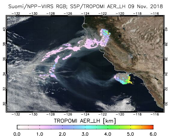
TROPOMI ATBD Aerosol Layer Height S5P-KNMI-L2-0006-RP
issue 2.2.0, 2021-07-05 – Released Page 8 of 75
9 Aerosol profile parameterizations for the TROPOMI Aerosol Layer Height product. (A) The
baseline profile parameterization assumes an elevated layer with a fixed pressure difference
between top and bottom of the layer. The layer’s mid pressure is retrieved. (B) If the aerosol
optical thickness is large enough, it will perhaps be possible to simultaneously fit the top
and bottom pressure. (C) An alternative parameterization that might be used, depending on
the aerosol case, assumes an aerosol layer extending down to the ground. The layer’s top
pressure is retrieved.. . . . . . . . . . . . . . . . . . . . . . . . . . . . . . . . . . . . . . . . . . . . . . . . . . . . . . . . . . . . . . . . . . . . . . . . . . . . . . 36
10 χ 2 of the (simulated) measurement (first term of Eq. 6) for an aerosol layer between 980 and
800 hPa with optical thickness of 0.3 at 550 nm over vegetated land. The measurement vector
y includes the O2 A band, or the O2 A and B bands. Note that the surface is much brighter in
the O2 A band. The modeled spectrum F(x) differs from the measurement with respect to
optical thickness. One can clearly see multiple minima in the cost function if only the O2 A
band is taken into account. . . . . . . . . . . . . . . . . . . . . . . . . . . . . . . . . . . . . . . . . . . . . . . . . . . . . . . . . . . . . . . . . . . . . . . . 37
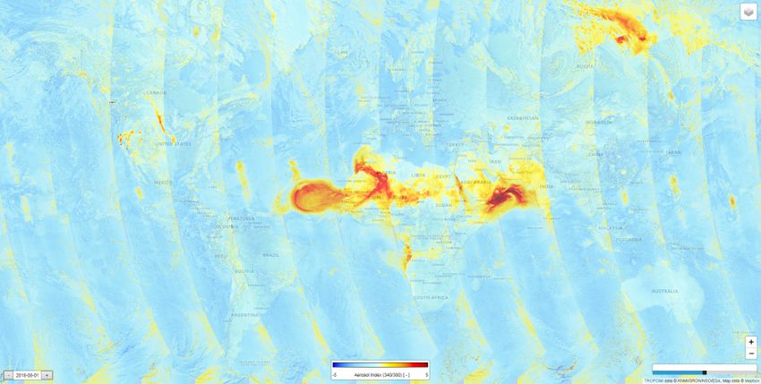
11 Top panel: TROPOMI AAI on 1 August 2018 showing a large aerosol (dust) plume over
the Atlantic Ocean originating from the Sahara, and several other hotspots of high AAI from
smoke and dust. Bottom panel: TROPOMI AER_LH retrieval results from an initial test run of
the ALH processor with NN implemented in the forward model. . . . . . . . . . . . . . . . . . . . . . . . . . . . . . . 38
12 Timeliness of the AER_LH processor. The upper panel shows the processing time per
near-real time granule. The bottom panel shows the timeliness of the end of the processing
time. ‘Large’ pixels refer to pixels with an integration time of 1080 ms, yielding pixel sizes of
7×7 km2 at nadir, ‘small’ pixels refer to an integration time of 840 ms, yielding pixel sizes of
about 7×5.6 km2 . . . . . . . . . . . . . . . . . . . . . . . . . . . . . . . . . . . . . . . . . . . . . . . . . . . . . . . . . . . . . . . . . . . . . . . . . . . . . . . . . . 39
13 Timeliness of the AER_LH processor. The top panel shows the difference in time spent by
the ALH processor with (black) and without (red) AAI filter in absolute time (minutes). The
relative difference is shown in blue. In the bottom panel the total number of pixels is shown in
red, and the fraction of pixels selected for different selection filters. In green the ’algorithm v1’
refers to the ALH algorithm which selected aerosol containing pixels on the basis of an AAI
> 0. This resulted in a low number of pixels. In black the fraction of pixels for the VIIRS cf
< 0.02 is shown, which selects up to 25% of the pixels for processing. In blue the criteria of
no sun glint but processing pixel with AAI> 1 is added. In purple the fraction of pixels for the
FRESCO effective cloud fraction < 0.02 AND AAI > 1 is shown. . . . . . . . . . . . . . . . . . . . . . . . . . . . . . 40
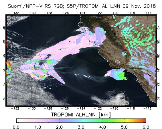
14 (top-left) Suomi/NPP VIIRS RGB on 9 Nov. 2018, overlaid with LBL ALH ; (top-right) Suomi/NPP
VIIRS RGB on 9 Nov. 2018, overlaid with NN ALH; (bottom-left)Suomi/NPP VIIRS RGB on
9 Nov. 2018, overlaid with difference of NN-LBL ALH; (bottom-right) Scatterplot of NN ALH
versus LBL ALH for the pixels in the left panels. . . . . . . . . . . . . . . . . . . . . . . . . . . . . . . . . . . . . . . . . . . . . . . . . 45
15 (left) Scatterplot of NN ALH versus LBL ALH on 10 Nov 2018 for the area in Fig 14; (right)
Same as the left panel for 11 Nov. 2018. . . . . . . . . . . . . . . . . . . . . . . . . . . . . . . . . . . . . . . . . . . . . . . . . . . . . . . . . 46
16 Precision of retrieved aerosol mid pressure as a function of mid pressure for three values of
the aerosol optical thickness. Panel A shows retrieval precision for an aerosol layer over sea /
ocean; Each of the four subplots in a panel corresponds to a different observation geometry:
SZA 25◦ , VZA 0◦ (top left); SZA 25◦ , VZA 70◦ , RAA 90◦ (top right); SZA 60◦ , VZA 0◦ (bottom
left); and SZA 60◦ , VZA 0◦ , RAA 90◦ (bottom right). Note the different scales of the x-axis.. 48
17 Precision of retrieved aerosol mid pressure as a function of mid pressure for three values
of the aerosol optical thickness. Panel A shows retrieval precision for an aerosol layer over
vegetated land. Each of the four subplots in a panel corresponds to a different observation
geometry: SZA 25◦ , VZA 0◦ (top left); SZA 25◦ , VZA 70◦ , RAA 90◦ (top right); SZA 60◦ , VZA
0◦ (bottom left); and SZA 60◦ , VZA 0◦ , RAA 90◦ (bottom right). Note the different scales of
the x-axis. . . . . . . . . . . . . . . . . . . . . . . . . . . . . . . . . . . . . . . . . . . . . . . . . . . . . . . . . . . . . . . . . . . . . . . . . . . . . . . . . . . . . . . . . . . 49
18 Precision of retrieved mid pressure as a function of surface albedo for three arbitrary atmo-
spheric states and observation geometries. . . . . . . . . . . . . . . . . . . . . . . . . . . . . . . . . . . . . . . . . . . . . . . . . . . . . . 50
19 Effect of a model error in the single scattering albedo on retrieved mid pressure and aerosol
optical thickness as a function of optical thickness. We assume a single scattering albedo
of 0.95 in retrieval, while the true single scattering albedo is either 0.90 (solid lines) or 1.0
(dashed lines). The aerosol layer is located at 600 hPa (green lines) or 800 hPa (red lines).
First row: bias in retrieved mid pressure; second row: precision of retrieved mid pressure;
third row: bias in retrieved optical thickness with error bars indicating precision. Panel A (left
column) shows retrieval simulations over sea / ocean; panel B (right column) shows retrieval
simulations over vegetated land. The x-axis has a logarithmic scale. . . . . . . . . . . . . . . . . . . . . . . . . . 52
TROPOMI ATBD Aerosol Layer Height                                                                                                                           S5P-KNMI-L2-0006-RP
issue 2.2.0, 2021-07-05 – Released                                                                                                                                  Page 9 of 75

20      Phase functions for the three aerosol models used in the retrieval simulations of Figure 21.
        The black line corresponds to a Henyey-Greenstein phase function with asymmetry parameter
        of 0.7, which is used in retrieval. . . . . . . . . . . . . . . . . . . . . . . . . . . . . . . . . . . . . . . . . . . . . . . . . . . . . . . . . . . . . . . . . .                     54
21      Effect of a model error in the phase function on retrieved aerosol pressure as a function of
        optical thickness for three values of aerosol pressure. Panel A (first row): ‘Dust over ocean’;
        panel B (second row): ‘Biomass burning over land’; panel C (third row): ‘Boundary layer
        pollution’. For details of these scenarios, see the text and Table 12. In each panel, the left plot
        shows the bias in retrieved aerosol pressure and the right plot shows precision of retrieved
        pressure. We assume a Henyey-Greenstein phase function with asymmetry parameter of 0.7
        in retrieval. Note that for the ‘Boundary layer pollution’ scenario, we assume an aerosol profile
        consisting of a single layer extending down to the ground surface. In this case, we retrieve the
        layer’s top pressure ptop . The x-axis has a logarithmic scale. . . . . . . . . . . . . . . . . . . . . . . . . . . . . . . . . . .                                                       56
22      Reflectance spectra for two different combinations of optical thickness and surface albedo
        that yield the same continuum reflectance. All other parameters are the same. The aerosol
        layer is between 540 and 475 hPa; the single scattering albedo is 1.0; the solar zenith angle
        is 25◦ and the viewing direction is nadir. From the shape of absorption we can simultaneously
        fit surface albedo and aerosol optical thickness. . . . . . . . . . . . . . . . . . . . . . . . . . . . . . . . . . . . . . . . . . . . . . . . .                                         57
23      Effect of an error in climatological albedo values on retrieved aerosol pressure as a function
        of the true surface albedo for three retrieval types (Table 13). Panel A (first row): aerosol layer
        with optical thickness of 0.5 at 500 hPa over sea / ocean; panel B (second row): aerosol layer
        with optical thickness of 0.5 at 800 hPa over vegetated land. In each panel, the left plot shows
        the bias in retrieved aerosol pressure and the right plot shows precision of retrieved pressure.
        The climatological surface albedo value, which is used in retrieval, is indicated by the arrow.
        Missing data points indicate that retrieval does not converge. . . . . . . . . . . . . . . . . . . . . . . . . . . . . . . . . .                                                          59
24      Effect of a model error in the single scattering albedo on the bias in retrieved pressure as a
        function of the true single scattering albedo for three retrieval types (Table 13). The single
        scattering albedo assumed in retrieval is 0.95. Left: aerosol layer with optical thickness of 0.5
        at 500 hPa over sea / ocean; right: aerosol layer with optical thickness of 0.5 at 800 hPa over
        vegetated land. Missing data points indicate that retrieval does not converge. . . . . . . . . . . . . . . .                                                                              60
25      Precision of retrieved aerosol pressure (left plot) and optical thickness (right plot) as a function
        of the a priori error in the temperature profile. The aerosol layer has optical thickness of 0.5
        and is located at 500 hPa (green lines) or 800 hPa (red lines), over sea / ocean (solid lines)
        or vegetated land (dashed lines). Retrieval precision shows the same behavior if the optical
        thickness is 0.2. . . . . . . . . . . . . . . . . . . . . . . . . . . . . . . . . . . . . . . . . . . . . . . . . . . . . . . . . . . . . . . . . . . . . . . . . . . . . . . . . . . .   61
26      Precision of retrieved aerosol pressure (left plot) and optical thickness (right plot) as a function
        of the a priori error in the surface pressure. The aerosol layer has optical thickness of 0.5
        and is located at 500 hPa (green lines) or 800 hPa (red lines), over sea / ocean (solid lines)
        or vegetated land (dashed lines). Retrieval precision shows the same behavior if the optical
        thickness is 0.2. . . . . . . . . . . . . . . . . . . . . . . . . . . . . . . . . . . . . . . . . . . . . . . . . . . . . . . . . . . . . . . . . . . . . . . . . . . . . . . . . . . .   62
27      Effect of an unscreened cloud layer on retrieved aerosol pressure for three values of the
        aerosol optical thickness. Left: cirrus layer between 330 and 300 hPa with cloud fraction 1.0
        and varying cloud optical thicknesses; right: cumulus cloud between 910 and 890 hPa with
        cloud optical thickness of 10 and varying cloud fractions. The aerosol layer is at 700 hPa over
        sea / ocean. The profile parameterization in retrieval assumes one scattering layer. Missing
        data points indicate that retrieval does not converge. . . . . . . . . . . . . . . . . . . . . . . . . . . . . . . . . . . . . . . . . . . .                                              64
28      Precision of retrieved profile parameters as a function of the a priori error in the surface
        albedo for the baseline profile parameterization of a layer with fixed pressure thickness and
        the alternative implementation of a layer with variable pressure thickness. Left: aerosol layer
        with optical thickness of 0.5 at 500 hPa over vegetated land; right: aerosol layer with optical
        thickness of 0.5 at 800 hPa over sea / ocean. The baseline algorithm fits mid pressure (green
        solid line) and the alternative implementation fits mid pressure and pressure thickness (red
        dashed lines). Note the logarithmic scale of the x-axis. . . . . . . . . . . . . . . . . . . . . . . . . . . . . . . . . . . . . . . . .                                                  65
29      Accuracy (left plot) and precision (right plot) of retrieved aerosol pressure as a function of
        optical thickness when the vegetated land surface exhibits chlorophyll fluorescence. Solid
        lines correspond to a retrieval in which fluorescence is present in the simulation but not
        accounted for in the forward model for retrieval. Dashed lines correspond to a retrieval in
        which fluorescence emissions are included in the forward model and retrieved simultaneously
        with aerosol parameters.. . . . . . . . . . . . . . . . . . . . . . . . . . . . . . . . . . . . . . . . . . . . . . . . . . . . . . . . . . . . . . . . . . . . . . . . . .               66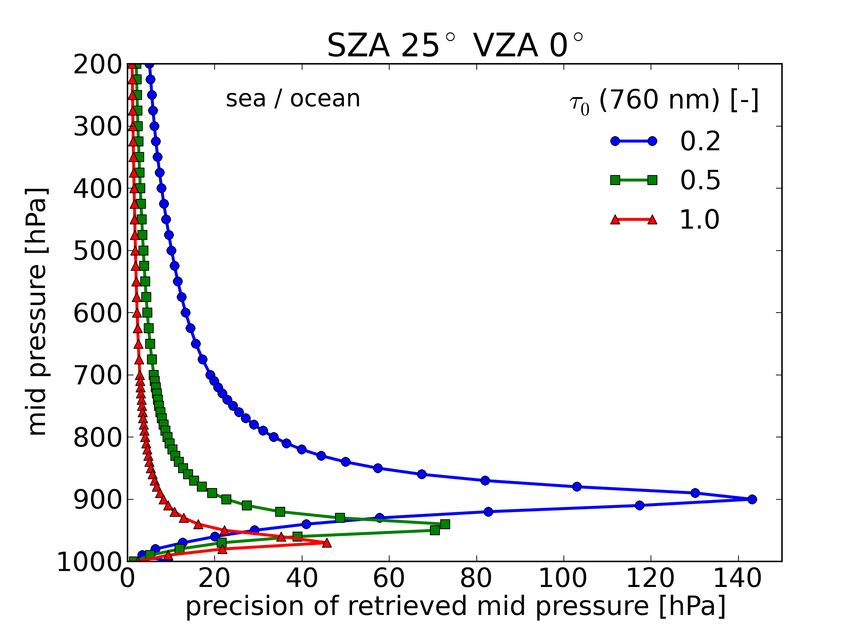
TROPOMI ATBD Aerosol Layer Height                                                                           S5P-KNMI-L2-0006-RP
issue 2.2.0, 2021-07-05 – Released                                                                                 Page 10 of 75

30       (top) Suomi/NPP VIIRS RGB on 10 Nov. 2018, overlaid with NN ALH. The yellow line depicts
         the CALIPSO track overpassing that day. The yellow dashed line depict the 20 km range
         around the CALIPSO track; (bottom) CALIOP Total attenuated backscatter at 532 nm on 10
         Nov. 2018 for the track shown by the yellow line in the top panel. . . . . . . . . . . . . . . . . . . . . . . . . . . . .   70
TROPOMI ATBD Aerosol Layer Height S5P-KNMI-L2-0006-RP issue 2.2.0, 2021-07-05 – Released Page 11 of 75 1 Introduction 1.1 Identification This document, identified as S5P-KNMI-L2-0006-RP, is the Algorithm Theoretical Basis Document (ATBD) for the Tropospheric Monitoring Instrument’s (TROPOMI) Aerosol Layer Height (ALH) product. It is part of a series of ATBDs describing the TROPOMI Level-2 products. 1.2 Purpose and objective The purpose of this document is to describe the current implementation and the theoretical basis of the Aerosol Layer Height algorithm. The document is maintained during the development phase and the lifetime of the data product. Updates and new versions are foreseen if there are changes to the algorithm. 1.3 Document overview Section 2 lists applicable and reference documents within the Sentinel-5 Precursor (S5P) / TROPOMI project as well as electronic references. Section 3 gives a list of terms, abbreviations and symbols that are specific for this document. Section 4, section 5 and section 6 describe the forward model and retrieval method, respectively. Section 7 discusses the operational algorithm’s feasibility. Section 8 provides an extensive error analysis. Section 9 presents a validation plan for the Aerosol Layer Height product. Section 10 provides a general conclusion and outlook. Finally, Section 12 lists references to peer-reviewed papers and other scientific publications. 1.4 Acknowledgements The authors would like to thank the following persons for useful discussions: Maarten Sneep, Gijs Tilstra, Ofelia Vieitez, Piet Stammes, Arnoud Apituley and Pepijn Veefkind.
TROPOMI ATBD Aerosol Layer Height                                                     S5P-KNMI-L2-0006-RP
issue 2.2.0, 2021-07-05 – Released                                                           Page 12 of 75

2     Applicable and reference documents
2.1   Applicable documents
[AD1] OMI Geolocation Review.
      source: KNMI; ref: TN-OMIE-KNMI-729; issue: 1.0; date: 2004-04-05.

[AD2] Science Requirements Document for TROPOMI. Volume I: Mission and Science Objectives and Obser-
      vational Requirements.
      source: KNMI, SRON; ref: RS-TROPOMI-KNMI-017; issue: 2.0.0; date: 2008-10-30.

2.2   Reference documents
 [RD1] Terms, definitions and abbreviations for TROPOMI L01b data processor.
       source: KNMI; ref: S5P-KNMI-L01B-0004-LI; issue: 3.0.0; date: 2013-11-08.

 [RD2] Terms and symbols in the TROPOMI Algorithm Team.
       source: KNMI; ref: S5P-KNMI-L2-0049-MA; issue: 1.0.0; date: 2015-07-16.

 [RD3] S5P/TROPOMI Science Verification Report.
       source: IUP; ref: S5P-IUP-L2-ScVR-RP; issue: 2.1; date: 2015-12-22.

 [RD4] TROPOMI Instrument and Performance Overview.
       source: KNMI; ref: S5P-KNMI-L2-0010-RP; issue: 0.10.0; date: 2014-03-15.

 [RD5] S5P-NPP Cloud Processor ATBD.
       source: RAL Space; ref: S5P-NPPC-RAL-ATBD-0001; issue: 1.0.0; date: 2016-02-12.

 [RD6] DISAMAR: Determining Instrument Specifications and Analyzing Methods for Atmospheric Retrieval,
       User Manual.
       source: KNMI; ref: RP-TROPOMI-KNMI-104; issue: -; date: 2012-02-08.

 [RD7] DISAMAR. Determining Instrument Specifications and Analyzing Methods for Atmospheric Retrieval.
       Algorithm description and background information.
       source: KNMI; ref: RP-TROPOMI-KNMI-066; issue: 2.2.1; date: 2011-05-19.

 [RD8] Calibration analysis report for TROPOMI UVN instrument spectral response function.
       source: KNMI; ref: S5P-KNMI-OCAL-0124-RP; issue: 0.1.0; date: 2015-10-01.

 [RD9] DISAMAR: Determining Instrument Specifications and Analyzing Methods for Atmospheric Retrieval,
       Algorithms and background.
       source: KNMI; ref: RP-TROPOMI-KNMI-066; issue: -; date: 2012-01-24.

[RD10] D. P. Dee, S. M. Uppala, A. J. Simmons et al.; The ERA-Interim reanalysis: configuration and per-
       formance of the data assimilation system. Quarterly Journal of the Royal Meteorological Society ; 137
       (2011) (656), 553; 10.1002/qj.828. URL https://rmets.onlinelibrary.wiley.com/doi/abs/10.1002/qj.
       828.
[RD11] K. Chance and R.L. Kurucz; An improved high-resolution solar reference spectrum for earth’s atmo-
       sphere measurements in the ultraviolet, visible, and near infrared. Journal of Quantitative Spectroscopy
       and Radiative Transfer ; 111 (2010) (9), 1289; 10.1016/j.jqsrt.2010.01.036.

[RD12] Wavelength calibration for S5P L2 data processors.
       source: KNMI; ref: S5P-KNMI-L2-0126-TN; issue: 1.0.0; date: 2015-09-11.

[RD13] DISAMAR: Determining Instrument Specifications and Analyzing Methods for Atmospheric Retrieval,
       Line Mixing and Collision Induced Absorption for the O2 A-band.
       source: KNMI; ref: RP-TROPOMI-KNMI-???; issue: -; date: 2012-01-24.

[RD14] Wavelength calibration in the Sentinel 5-precursor Level 2 data processors.
       source: KNMI; ref: S5P-KNMI-L2-0126-TN; issue: 1.0.0; date: 2015-09-11.

[RD15] Preparing elevation data for Sentinel 5 precursor.
       source: KNMI; ref: S5P-KNMI-L2-0121-TN; issue: 2.0.0; date: 2015-09-11.
TROPOMI ATBD Aerosol Layer Height S5P-KNMI-L2-0006-RP
issue 2.2.0, 2021-07-05 – Released Page 13 of 75
[RD16] Algorithm theoretical basis document for the TROPOMI L01b data processor.
source: KNMI; ref: S5P-KNMI-L01B-0009-SD; issue: 6.0.0; date: 2015-09-22.
2.3 Electronic references
[ER1] URL https://www.tensorflow.org.
[ER2] URL http://temis.nl/surface/.
[ER3] URL http://www.cfa.harvard.edu/hitran/.
[ER4] URL http://www.esa-aerosol-cci.org.TROPOMI ATBD Aerosol Layer Height S5P-KNMI-L2-0006-RP
issue 2.2.0, 2021-07-05 – Released Page 14 of 75
3 Terms, definitions and abbreviated terms
Terms, abbreviations and symbols that are used within the TROPOMI Level-2 project are described in [RD1].
and [RD2]. Terms, definitions and abbreviated terms that are specific for this document can be found below.
More in [AD1]
3.1 Terms and definitions
accuracy systematic error component
height vertical height, either in units of hPa (pressure) or in units of km (altitude)
hyperspectral imager imager with large number of spectral channels, often at high spectral resolution
(better than about 0.5-1 nm), e.g. GOME-2
multispectral imager imager with a number of spectral channels (typically 30-50) that are generally
not contiguous and have coarser spectral resolution (2-10 nm), e.g. MODIS
3.2 Acronyms and Abbreviations
UVAI UV Aerosol Index
AERONET Aerosol Robotic Network
AEROPRO Aerosol Profile Retrieval Concept Development and Validation for Sentinel-4
ALH Aerosol Layer Height
ATBD Algorithm Theoretical Basis Document
AVHRR Advanced Very High Resolution Radiometer
BSA black-sky albedo
CALIOP Cloud-Aerosol Lidar with Orthogonal Polarisation
CALIPSO Cloud-Aerosol Lidar and Infrared Pathfinder Satellite Observation
CIA collision-induced absorption
CPU central processing unit
DISAMAR Determining Instrument Specifications and Analyzing Methods for Atmo-
spheric Retrieval
DLR Deutsches Zentrum für Luft- und Raumfahrt
DWD Deutscher Wetterdienst
EarthCARE Earth Clouds, Aerosols and Radiation Explorer
ECMWF European Centre for Medium-Range Weather Forecasts
EARLINET European Aerosol Research Lidar Network
ERA ECMWF Reanalysis
FRESCO Fast Retrieval Scheme for Clouds from the Oxygen A Band
FWHM full width at half maximum
GALION GAW Atmospheric Lidar Observation Network
GMES Global Monitoring of the Environment and Security
GOME Global Ozone Monitoring Experiment
GOSAT Greenhouse Gases Observing Satellite
HALO High Altitude and Long Range Research Aircraft
HG Henyey-Greenstein
HITRAN High Resolution Transmission
HSRL High Spectral Resolution Lidar
IASI Infrared Atmospheric Sounding Interferometer
IUP Institut für Umweltphysik
JPL Jet Propulsion Laboratory
KNMI Koninklijk Nederlands Meteorologisch InstituutTROPOMI ATBD Aerosol Layer Height S5P-KNMI-L2-0006-RP
issue 2.2.0, 2021-07-05 – Released Page 15 of 75
LABOS layer-based orders of scattering
LBL Line-by-line
LER Lambertian-equivalent reflectivity
LM line mixing
MERIS Medium Resolution Imaging Spectrometer
MetOp Meteorological Operational Satellite
MISR Multi-Angle Imaging Spectroradiometer
MLS mid-latitude summer
MODIS Moderate Resolution Imaging Spectroradiometer
MTG-S Meteosat Third Generation - Sounder
NIR near infrared
NN neural network
NSIDC National Snow & Ice Data Center
OMI Ozone Monitoring Instrument
PMD Polarisation Measurement Devices
POLDER Polarization and Directionality of the Earth’s Reflectance
RAA relative azimuth angle
S5P Sentinel-5 Precursor
S/C spacecraft
SACURA Semi-Analytical Cloud Retrieval Algorithm
SCIAMACHY Scanning Imaging Absorption Spectrometer for Atmospheric Cartography
SNR signal-to-noise ratio
Suomi-NPP Suomi National Polar-orbiting Partnership
SWIR shortwave infrared
SZA solar zenith angle
TANSO-FTS Thermal and Near Infrared Sensor for Carbon Observations Fourier-Transform
Spectrometer
TROPOMI Tropospheric Monitoring Instrument
UV ultraviolet
UVIS ultraviolet-visible
UVN ultraviolet-visible-near infrared
VCM VIIRS cloud mask
VIIRS Visible / Infrared Imaging Radiometer Suite
VIS visible
VZA viewing zenith angleTROPOMI ATBD Aerosol Layer Height S5P-KNMI-L2-0006-RP issue 2.2.0, 2021-07-05 – Released Page 16 of 75 3.3 Symbols ω0 single scattering albedo [-] τ0 aerosol or cloud optical thickness [-] α Ångström coefficient [-] g asymmetry parameter [-] pmid aerosol mid pressure [hPa] zmid aerosol mid altitde [km] ptop aerosol top pressure [hPa] ∆p pressure thickness [hPa] ps surface pressure [hPa] zs surface altitude (above reference surface) [km] As surface albedo [-] Fs surface (fluorescence) emission [ph. cm−2 s−1 nm−1 sr−1 ]
TROPOMI ATBD Aerosol Layer Height                 S5P-KNMI-L2-0006-RP
issue 2.2.0, 2021-07-05 – Released                       Page 17 of 75

 R           Reflectance [sr−1 ]
 I           Radiance [ph. cm−2 s−1 nm−1 sr−1 ]
 E0          Irradiance [ph. cm−2 s−1 nm−1 ]
TROPOMI ATBD Aerosol Layer Height                                                       S5P-KNMI-L2-0006-RP
issue 2.2.0, 2021-07-05 – Released                                                             Page 18 of 75

4     Introduction to Aerosol Layer Height product
4.1   Product description
The Tropospheric Monitoring Instrument features a new aerosol product that is dedicated to retrieval of the
height of tropospheric aerosols. Before the launch of TROPOMI, daily global observations of aerosol height
were not available on an operational basis. Aerosol profiles were provided by active sensors, particularly by
ground-based lidar systems or by the space-borne Cloud-Aerosol Lidar with Orthogonal Polarisation (CALIOP),
and aerosol layer height by multi-angle sensors, most notably Multi-Angle Imaging SpectrRadiometer (MISR).
Active sensors have a high vertical resolution, but CALIOP and MISR observe in narrow tracks only. However,
passive sensors, such as TROPOMI, can cover the entire earth in a single day.
    The TROPOMI Aerosol Layer Height product focuses on retrieval of vertically localized aerosol layers in
the free troposphere, such as desert dust, biomass burning aerosol, or volcanic ash plumes. The height of
such layers is retrieved for cloud-free conditions. Height information for aerosols in the free troposphere is
particularly important for aviation safety. Scientific applications include radiative forcing studies, long-range
transport modeling and studies of cloud formation processes. Aerosol height information also helps to interpret
the UV Aerosol Index (UVAI) in terms of aerosol absorption as the index is strongly height-dependent.
    Retrieval of aerosol height is based on absorption by oxygen in the A band. The O2 A band is located in
the near-infrared wavelength range between about 759 and 770 nm. It is a highly structured line absorption
spectrum with strongest absorption lines occurring between 760 and 761 nm. The absorption band spans a
wide range of absorption optical thicknesses. At some wavelengths, photons do not reach the lower levels of
the atmosphere.
    Figure 1 shows simulated reflectance spectra at TROPOMI’s anticipated instrument specifications (as
described in [56]) for an aerosol layer at two different pressures. The difference between the two spectra

Figure 1: Simulated reflectance spectra of the O2 A band at a spectral resolution (FWHM) of 0.5 nm for a
scene containing a representative aerosol layer. The aerosol layer is between 950 and 850 hPa (green line) or
between 540 and 475 hPa (blue line). The 1-σ measurement errors on reflectance are smaller than the width
of the plotting lines: anticipated signal-to-noise ratios for these spectra (based on [56]) are about 645 in the
continuum and 302 and 207 in the deepest part of the O2 A band assuming pure shot noise. The solar zenith
angle is 25◦ and the viewing direction is nadir. The aerosol optical thickness τ 0 at 550 nm is 1.0, the Ångström
coefficient α is 2.0, the single scattering albedo is 1.0, and the phase function is a Henyey-Greenstein function
with asymmetry parameter g of 0.7. Spectra were simulated with a temperature profile corresponding to the
mid-latitude summer (MLS) atmosphere, a surface pressure of 1013 hPa and a constant ground surface albedo
of 0.025.
TROPOMI ATBD Aerosol Layer Height S5P-KNMI-L2-0006-RP
issue 2.2.0, 2021-07-05 – Released Page 19 of 75
Figure 2: Schematic depiction of the atmosphere and typical TROPOMI satellite configuration for retrieval of
Aerosol Layer Height. The Rayleigh scattering optical thickness at the O2 A band is ~0.02
.
provides the aerosol pressure signal. The baseline fit window for the Aerosol Layer Height algorithm extends
from 758 nm (continuum) to 770 nm. For more recent TROPOMI instrument specifications, see . A schematic
depiction of the satellite configuration for observations of the O2 A band with TROPOMI is given in Figure 2.
4.2 Heritage
TROPOMI Aerosol Layer Height is a new operational Level-2 product. Heritage products for an operational
aerosol profile retrieval based on hyperspectral measurements of the oxygen A band presently do not exist.
However, the Aerosol Layer Height algorithm can be applied to measurement series from the Scanning Imaging
Absorption Spectrometer for Atmospheric Cartography (SCIAMACHY; [3]) and the Global Ozone Monitoring
Experiment-2 (GOME-2). A first case study of ALH retrieval with GOME-2 measurements has been published
as [43]. Aerosol Layer Height retrievals were performed for a number of aerosol scenes covering various
aerosol types, both elevated and boundary layer aerosols and land and sea surfaces. The retrieval results
were evaluated with lidar measurements. A follow-up study applied the TROPOMI ALH algorithm to desert
dust outbreaks off the West African coast observed with SCIAMACHY. Within the TROPOMI project also a
scientific verification study of the prototype algorithm has been performed. An independent ALH verification
algorithm from the Institute of Environmental Physics (IUP, Bremen, Germany) and the prototype ALH algorithm
from KNMI were applied to the case of a volcanic ash plume near Iceland observed with GOME-2 (chapter
14 in [RD3]). Retrieval results were intercompared and evaluated with plume heights retrieved with MISR
(stereoscopic retrieval). The main conclusions from these studies have been included in this ATBD as much as
possible. Finally, we remark that the TROPOMI Aerosol Layer Height algorithm will serve as the ALH heritage
algorithm for the future Sentinel–4 and Sentinel–5 missions [24], which make hyperspectral observations of the
O2 A band as well.
Early papers investigating the O2 A band for aerosol retrieval are by Badayev and Malkevich (1978)[2] and
Gabella et al. (1999) [2] and [17]. Corradini and Cervino (2006) [8] present a simulation study of retrieval of the
extinction profile for SCIAMACHY instrument characteristics with all other parameters (e.g. aerosol and surface
properties) being assumed in retrieval. Actual case studies exploiting hyperspectral O2 A band measurements
have been performed by Koppers and Murtagh (1997) [31] for GOME data, and by Kokhanovsky and Rozanov
(2010) [30] and Sanghavi et al. (2012) [46] for SCIAMACHY data. Koppers and Murtagh (1997) retrieve surface
albedo simultaneously with aerosol optical thickness and height distribution, while in the retrievals proposed
by Kokhanovsky and Rozanov (2010) and Sanghavi et al. (2012) the surface albedo basically is a modelTROPOMI ATBD Aerosol Layer Height S5P-KNMI-L2-0006-RP
issue 2.2.0, 2021-07-05 – Released Page 20 of 75
parameter (i.e. surface albedo not fitted). A retrieval setup similar to Kokhanovsky and Rozanov (2010) is being
extended to GOME-2 case studies [33]. Sensitivity studies to consolidate instrument requirements for O2 A
band aerosol retrieval include studies by Siddans et al. (2007) [47] and Hasekamp and Siddans (2009) [20]
for Sentinel–4/5, and by Hollstein et al. (2012) [22] for the Earth Explorer 8 mission Fluorescence Explorer
(FLEX). Dubuisson et al. (2009) [14] present a method to retrieve the altitude of aerosol plumes over ocean
from the ratio of reflectances in the two O2 A band channels of the Medium Resolution Imaging Spectrometer
(MERIS) and the Polarization and Directionality of the Earth’s Reflectance (POLDER) instrument. Finally, we
mention the work by Van Diedenhoven et al. (2005) [53] who showed that retrieved apparent surface pressure
(i.e. retrieved surface pressure when ignoring aerosol scattering) with SCIAMACHY depends systematically
on aerosol parameters. This illustrates in yet another way that the O2 A band contains aerosol information
available for retrieval.
Absorption by oxygen in the A band has been or is being used in operational cloud retrieval for the GOME
instruments (Fast Retrieval Scheme for Clouds from the Oxygen A Band (FRESCO) [28]) and for SCIAMACHY
(Semi-Analytical Cloud Retrieval Algorithm (SACURA)[40]). There are indications that the FRESCO cloud
retrieval algorithm may also provide information on aerosols in case of optically thick aerosol layers (Wang
et al., 2012) [57]. However, FRESCO uses a Lambertian surface to model cloud layers, which may be an
inaccurate approximation for aerosol layers since typical aerosol layers have significant transmission. The
forward model of the Aerosol Layer Height algorithm is developed specifically for retrieval of aerosol height.
Finally, we remark that the O2 A band is often used for an atmospheric scattering correction as part of more
convolved trace gas retrieval algorithms (e.g. [36] [5]; [38]; [58]).
4.3 Product requirements
Science requirements for the Aerosol Layer Height product are described in [AD2]. The target requirement on
the accuracy and precision of retrieved Aerosol Layer Height is 0.5 km or 50 hPa. The threshold requirement on
accuracy and precision is 1 km or 100 hPa. A minimum aerosol optical thickness for which these requirements
should be met is not specified. Note that an accuracy and precision requirement is defined for retrieved aerosol
height but not for retrieved aerosol optical thickness.
Furthermore, the Aerosol Layer Height product will be delivered in near real-time, which means that Level-2
data should be available within three hours after observation.
4.4 Overview of the retrieval algorithm
The Aerosol Layer Height algorithm presently has the following key features:
• Spectral fit estimation of reflectance across the O2 A band (wavelengths ~758–770 nm) using a neural
network;
• Retrieval method is Optimal Estimation;
• Main fit parameters are: aerosol layer mid pressure (pmid ) and aerosol optical thickness (τ 0 );
• Error estimates are provided to improve the usability of the product;
• Assumed aerosol profile: single uniform scattering layer with a fixed pressure thickness.
We assume that aerosols are confined to a single layer with a fixed pressure difference between top and bottom
of the layer, and with a constant aerosol volume extinction coefficient and aerosol single scattering albedo within
the layer. This parameterization is most suited for aerosol profiles that are dominated by a single, elevated,
optically thick aerosol layer. The product’s name explicitly refers to this particular profile parameterization. The
reported height parameter is the mid pressure of the layer defined as the sum of top pressure and bottom
pressure divided by two. The aerosol layer mid pressure (pmid ) is converted into an aerosol layer mid altitude
(zmid ) using an appropriate temperature profile. In addition to aerosol layer mid pressure, also the aerosol
optical thickness is retrieved. The retrieved aerosol optical thickness holds for wavelengths of the O2 A band
(i.e. at 760 nm). The wavelength range of the O2 A band is too small to provide information on the spectral
dependence of the optical thickness. The Aerosol Layer Height product contains error estimates as well as
other relevant diagnostics so that the user can evaluate the retrieval result.
From retrieval simulation experiments and a validation study for SCIAMACHY ALH retrievals, we have
learned that the retrieved mid pressure of the assumed aerosol layer can in general be regarded as an average
aerosol scattering height.TROPOMI ATBD Aerosol Layer Height S5P-KNMI-L2-0006-RP
issue 2.2.0, 2021-07-05 – Released Page 21 of 75
Figure 3: Flow chart for the Aerosol Layer Height retrieval algorithm.
The baseline fit window extends from 758 to 770 nm and covers the entire O2 A band. The error analysis
reported in Section 8 is performed for this fit window so that it provides a benchmark against which alternative
implementations can be compared.
A basic flow chart of the algorithm is given in Figure 3. Calibrated radiances, irradiances and their
associated measurement errors are the main inputs for the algorithm. Initially, cloud contaminated pixels are
excluded from the aerosol layer height retrieval. Additionally, pixels covered by snow or (sea) ice or in the
sunglint region are initially excluded from analysis as well. However, in order to process pixels that contain
thick plumes of aerosols that may be mistaken for clouds, pixels are selected based on the UV Aerosol Index.
High values for this index indicate elevated absorbing aerosol plumes. Often, these are screened by cloud
filters. This may be the case for volcanic ash plumes, thick desert dust plumes and pyrocumulus smoke plumes.
To avoid the screening by cloud masks, all pixels with a sufficiently high UV aerosol index are included for
processing. Dynamic input data further comprise meteorological data. Static input includes oxygen absorption
parameters, a high-resolution solar irradiance spectrum, slit functions for the radiance and irradiance, and
surface altitude (digital elevation model). Finally, a surface albedo climatology is used to provide a priori values
for retrieval.
Aerosol optical properties show a large variation in time and space. However, the forward model used in
operational retrieval assumes a single, average aerosol model (e.g. single scattering albedo ω 0 of 0.95 and
Henyey-Greenstein phase function with asymmetry parameter g of 0.7). Sensitivity analyses for the Aerosol
Layer Height algorithm (Section 8) and experiments with GOME–2 spectra [44] have shown that a single,
fixed aerosol model is sufficient for a reasonably accurate (i.e. compared to science requirements) retrieval
of aerosol pressure, which is the primary objective of this product. We remark that retrieved aerosol optical
thickness holds for the particular aerosol model assumed in retrieval (phase function and single scattering
albedo) and should thus be understood as an effective quantity in this respect.
Development of the operational Aerosol Layer Height algorithm is ongoing work. In this document, the most
recent implementation of the operational algorithm is described. Updates and new versions of the ATBD are
foreseen during the development phase and the lifetime of the product when there are significant changes to
the algorithm. The current implementation of the algorithm is based on a neural network forward model and an
optimal estimation scheme in the retrieval. A detailed description of the Aerosol Layer Height retrieval algorithm
is given in Section 5.2 and Section 6. The sensitivity analyses presented in Section 8 illustrate the algorithm’s
expected performance and provide further support to the choices we made in the design of the algorithm.TROPOMI ATBD Aerosol Layer Height S5P-KNMI-L2-0006-RP
issue 2.2.0, 2021-07-05 – Released Page 22 of 75
Figure 4: Difference in coverage due to the selection of all cloud-free pixels (right panel) instead of selecting
only pixel with a UV-AI index >1 (left panel).
4.5 Updates
The current version 2.2.0 differs considerably from version 1.x. The main difference is the change from selecting
a limited set of pixels with absorbing aerosols, using the UV-AI product, to a product that generally processes
all cloud-free pixels.
The main reasons for abandoning the UV-AI selection are the availability of a new accurate cloud mask
from VIIRS, the degradation of the UV-AI and the development of the very fast NN forward model. These
developments allowed for the processing of a much larger number of pixels within the NRTI requirements,
therefore all cloud-free pixels are now processed. Hence not only absorbing aerosols are now being processed
but also scattering aerosol layers. Furthermore, the UV-AI signal was degrading, which yielded an increasingly
smaller number of selected pixels with absorbing aerosols. Although the degradation is corrected for in version
2.2.0, the selection by UV-AI is now abandoned. In Figure 4 the large change in pixel selection is shown
between v1 and v2 data.
The VIIRS cloud mask is not available in NRTI, therefore the FRESCO cloud product is used in NRTI. In
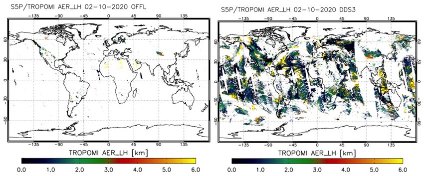
Figure 5 the change between the pixels masked by the NRTI cloud mask and the OFFL cloud mask is shown
for an orbit on 21 Sept. 2019. See section 5.1.1 for details on the cloud masks. The higher number of pixels
that need to be processed have a consequence on the timeliness of the processor, which is described in
section 7.1.
Figure 5: Difference in cloud masking between the NRTI processor (using FRESCO as a cloud mask) and the
OFFL cloud processor (using VIIRS as a cloud mask).You can also read