UVIS FLAT FIELDS AFFECTED BY SHUTTER-INDUCED VIBRATION - STSCI
←
→
Page content transcription
If your browser does not render page correctly, please read the page content below
Instrument Science Report 2018-11

                        UVIS Flat Fields Affected by
                          Shutter-Induced Vibration

                                                          H. Kurtz, P. R. McCullough, S. Baggett

                                                                                       August 8, 2018

Abstract
Image ratios of short internal tungsten flat fields exhibit faint diagonal striping along a
direction coincident with the shutter edge travel. We investigate the phenomenon using
additional archival data, both internal and external, and develop a model to quantify the
amount of variation observed across the field of view. We find 1) no evidence for striping
in external images, 2) the stripes are limited to short (< 10s) internal exposures and 3) the
stripes’ amplitude is noticeably higher in images taken with the B shutter blade.
Specifically, blade A image striping is typically 0.1% or less peak to peak while the blade B
striping is typically 0.5% or higher peak to peak for 1 s exposures. We interpret the lack of
striping in external images as an indication that the effect is not directly related to the
low-level blurring of the PSF observed in short (< 10s) external exposures that has been
attributed to shutter-induced vibrations of the WFC3 pick-off mirror or the M1 mirror.
Instead, we interpret the striping effect as a shutter-induced vibration of an optical element
in the internal light path of the calibration subsystem.

1     Introduction
   The Wide Field Camera 3 (WFC3) UVIS channel has a duplicate of the ACS WFC
shutter design. This is a disk consisting of two closed and two open sections referred to as
shutter A and B (Figure 1). The shutter (rotating disk) sits between the filter wheel and
the CCD housing and is mechanically and electronically capable of rotating both clockwise
and counter clockwise. However, the flight software rotates the shutter in only one direction.

Copyright c 2018 The Association of Universities for Research in Astronomy, Inc. All Rights Reserved.
Instrument Science Report 2018-11

The effect is the blade sweeps across the field of view from the corner of amplifier D in the
lower right up to the corner of amplifier A in the upper left (Sahu et al. 2015).

Figure 1: Sketch of the WFC3 UVIS shutter. The ‘beam foot-print’ is indicated (figure from
Baggett, 2003).

    We assess the possible contribution of the shutter behavior on the UVIS photometric
results. For example, in ISR 2017-15, aperture photometry of staring mode observations of
white dwarf standards (GD153 and GRW70) as a function of time and wavelength show 2-3
times the expected scatter over short timescales (Figs 8-10). In ISR 2017-21, photometry of
spatial scans of white dwarf standards – scaning mode provides significantly higher signal-
to-noise than staring mode. Most observations show excellent results yet some data show
2-3 times the expected scatter. That is, neither staring nor scanning mode routinely achieve
the expected short-term photometric scatter, i.e. results within the nominal error budget
(based on propagated errors from Poisson statistics and calibration files). This discrepancy
raises the question of whether the shutter behavior may be introducing some uncertainty
into the photometric results.

2    Data
    For our investigation we use archival data consisting of a large number of short internal
tungsten flat fields. These images are an ideal dataset to assess the shutter performance, as
they provide fine time sampling (every 0.5 - 3 days). We supplement this data with other,
less frequently acquired data such as deuterium flats, Earth flats, and external images, to

                                             2
Instrument Science Report 2018-11
see if the corrugation of internal flat field ratios is related to the shutter vibrations (chatter)
or e.g. lamp vibrations (stroboscopic) effect.
Source Proposal Title Proposal IDs ISRs
Tungsten UVIS Bowtie Monitoring 11908, 12344, 12688, 13072, ISR 2013-09
13555, 14001, 14367, 14530
Deuterium UVIS Internal Flats 11428, 11432, 11912, 12711, ISR 2016-05
13097, 13586, 14028, 14390, 14547
Earth Flat UVIS Earth Flats 12710, 11914 ISR 2013-10
Jupiter The Jovian Transit ... 13067 N/A
Mars MARS-OPPOSITION 14499, 15456 N/A
Table 1: Proposals for the data used in our analysis.
2.1 Tungsten Flats
The tungsten flats originate from a bowtie monitoring program used to prevent hysteresis
on the UVIS detector. This is accomplished via frequent short, 3-image visits. The first image
is a 1 second flat to detect if any hysteresis is present. The second image is a 200 second
flat that intentionally saturates the detector in order to neutralize any hysteresis. The final
image is a 1 second flat used to verify that the hysteresis has been removed. All of these
images are taken in 3x3 binned mode. A three image visit was taken every 3 days in 2017
(more frequently in the past), for a total of 3,984 images spanning June 2009 - October 2017.
We examine the 1-second images as ratios both to one another (i.e., for each visit, image 3
compared to image 1) and to representative reference images from 2012 (i.e. image 1 from
a visit compared back to a 2012 image 1, image 3 from a visit compared back to a 2012
image 3). The ratios normally serve as a test for whether the hysteresis, if present, has been
neutralized but for our study, we use the ratios to assess the shutter performance. These
images have a signal to noise of ∼ 10, 000 -e.
2.2 Deuterium Flats
The deuterium flats are chosen from the UVIS Internal Flats calibration proposals used
to monitor the stability of the UV filters and to check the flat field structure. We select
only flats with short exposure times (3.4s) because the shutter effect is attenuated in longer
exposures. This yields 23 deuterium flats (filter F200LP) from the proposals listed in Table
1. These flats have an average of 22,000 -e/pixel.
2.3 Earth Flats
Earth flats as the name implies, are observations of the Earth, chosen from the UVIS
Earth Flats program. The original intent of the Earth Flats was to check the filters and to
validate the L-flat solution. Here we employ the short exposure time (less than 5s) Earth
3Instrument Science Report 2018-11
flats as an external check of the shutter behavior. We examine a total of 140 Earth flats
in filters F656N, F469N, F336W, F343N, F373N, F395N, F390M. Of the 140 flats, 98 have
high signal to noise (greater than ∼ 10, 000 -e) and half of those were observed using shutter
B. Table 2 is a summary of the Earth flats examined, giving their exposure time and the
number of observations at that exposure time.
Exposure Time (s) Number of Observations Number of Observations with high signal to noise
0.48 16 12
0.8 16 11
0.9 12 8
1.0 64 41
1.7 12 12
1.9 4 4
4.1 12 7
4.6 4 3
Table 2: Earth flat data used in our analysis.
2.4 Jupiter Images
For a second external illumination source, an extended target with good signal to noise
in a short exposure time, we chose Jupiter. These Jupiter images are not ideal as they are
sub-arrays, however, other targets (e.g. other planets) did not sufficiently fill the field of
view or were too faint (e.g. sky flats). The Jupiter observations are taken from the Jovian
Transit of Venus program. We examine the data taken with filter F763M as those images
have exposure times of 0.48s. In total we examine 63 images of Jupiter.
2.5 Mars Images
An additional external source we examine is Mars. The Mars images were taken on a
sub-array of a small section of the detector. These images were taken from proposals 14499
and 15456 in 2016 and 2018 respectively. We use data taken in filters F673N and F410M
with an exposure time of 0.48s. In total we examine 11 images.
2.6 Moon Images
We also examined images of the Moon from proposal 12537. Of the 20 images only 3
were able to be examined due to lost guide stars and variations in the observed field. The
3 images each have an exposure time of 0.48s and are observed with filter F502N. We had
to align these images to one another before we could ratio them. The images had to be
translated and rotated to align. Because of slight misalignments and changes of the trailed
PSF, lunar features did not divide well, so we were therefore unable to see if corrugations
were present.
4Instrument Science Report 2018-11
3 Analysis
3.1 Tungsten Flats
We analyze tungsten flat image ratios from the bowtie monitoring program. Figure 2
shows a typical tungsten flat, illustrating the lamp illumination pattern (brighter in lower
right and dimmer in the upper left), the chip gap, dust specks, and a few bad pixels. Figure
3 shows the ratio of two tungsten flats with contours. The illumination pattern ratios out
but we are left with diagonal stripes, which align along the direction of the shutter blade
motion. We look at ratios of flats taken with shutter A to those with shutter B as well as
ratios of shutter A to A and shutter B to B. Of the images compared to a shutter B image
65% of them show the visible corrugation at a level of ∼Instrument Science Report 2018-11
Figure 2: A typical full frame internal 3X3 binned tungsten flat field. The grey scale is
+/- 10%, where white is high signal. Amps A and B are at the upper left and upper right
corners respectively; amps C and D are at the lower left and lower right respectively. The
same image orientation is used consistently throughout the ISR unless noted otherwise.
6Instrument Science Report 2018-11
Figure 3: A typical tungsten bowtie ratio with over-plotted contours. The grey scale is +/-
2.5%, where white is high signal.
7Instrument Science Report 2018-11
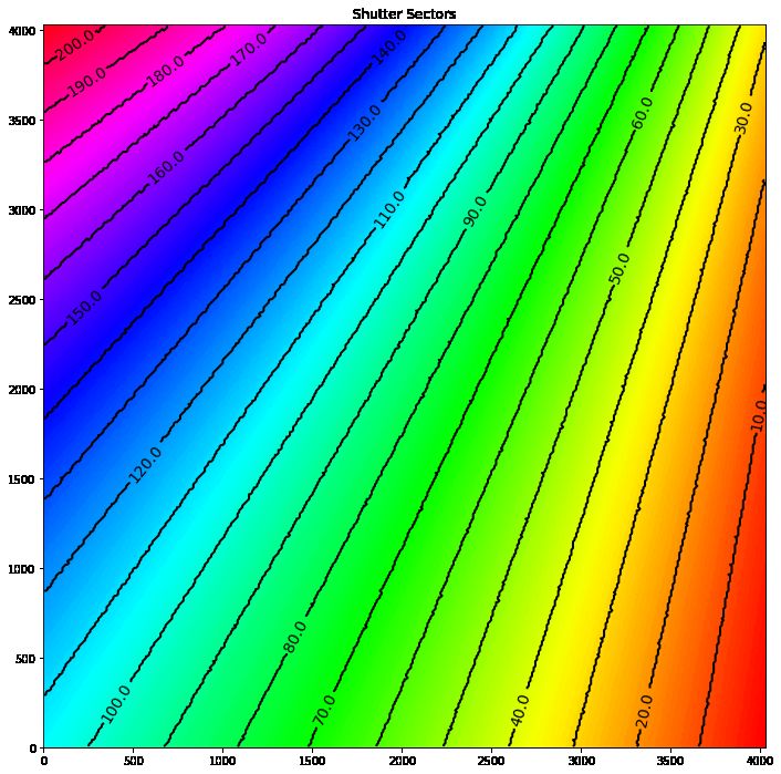
Figure 4: Map of the shutter sectors. The model motion of the shutter across the detector
is based on a 3x3 binned images from bowtie observations. Each sector is approximately 1.6
arcsec. The color shows the model motion as a gradient.
8Instrument Science Report 2018-11
Shu$er A ibct1w/q_ibct1w2q Shu$er B ibct25clq_ibct25cnq
Chip 1 Chip 1
Chip 2 Chip 2
Ra:o
Ra:o
Sector Number Sector Number
Figure 5: Median within shutter sectors across the detector as a function of sector number.
3.2 Deuterium Flats
WFC3 has two lamps in the calibration system, tungsten and deuterium, for visible and
UV flats respectively. Given the corrugation seen in the tungsten image ratios, we inspected
image ratios taken with the deuterium calibration lamp to see if the corrugations are present
there as well. Figure 6 shows a typical deuterium flat. These flats have more features than
the tungsten flats. Here we see the crosshatch pattern (from the manufacturing process) and
the dark spot in lower left, which is attributed to something on the housing of the deuterium
lamp (Rajan et al., 2010). Figure 7 is a typical ratio of two deuterium flats along side a
ratio of two deuterium flats which show the corrugation. Even with the features unique to
the deuterium lamp, a clear signature of the corrugation is visible. Three of 23 (13%) of
deuterium ratios show evidence of corrugation at a level we could discern (∼ 0.2%).
9Instrument Science Report 2018-11
Figure 6: Typical full frame deuterium flat field. The gray scale is +/- 5%, where white is
high signal. Amps A and B are at the upper left and right corners respectively; amps C and
D are at the lower left and right respectively.
10Instrument Science Report 2018-11
Figure 7: The left is a typical deuterium flat ratio and the right is the ratio of
iaan08o1q flt.fits and iaan05hbq flt.fits with the contours over-plotted. Corrugations typ-
ically are not evident (left) but sometimes are (right) in deuterium flat ratios. The gray
scale is +/- 1.5%, where white is high signal.
3.3 Earth Flats
Given that images with both types of calibration lamps exhibit the corrugations, we
investigated external images. If the corrugation is due to a common element present in both
internal and external light paths, we would expect at least 5-10% of short external exposures
to show the corrugations, based on their longer exposure time, their S/N and because of
small number statistics.
We start with Earth flats; a typical one is shown in Figure 8. Earth flats can have parallel
streaks in the image from the scene of Earth moving across the detector. Figure 9 shows
the ratio of two Earth flats; this ratio is relatively featureless except for some of the streaks.
Although in a similar direction as the tungsten and deuterium corrugations these streaks
in the ratio are not the same effect, because the streaks are parallel to the direction of the
spacecraft motion (green arrow). Also the streaks are all parallel to each other, whereas the
shutter effect is as in Figure 4 nearly vertical at lower right to nearly horizontal at upper
left.
About 50% of the Earth flat images we examine have streaks. We form the image ratios
using a relatively streak-free image in the denominator. Inspection of the image ratios shows
many with streaks in a direction inconsistent with the internal corrugation pattern. For
the ratios with streaks in the direction of the corrugation we over plot on the image ratios
11Instrument Science Report 2018-11
parallel lines along the direction of the spacecraft’s motion. In this manner we rule out
any Earth flats as having corrugations like the internal flat ratios, implicating a calibration
system component as the cause of the corrugations.
Figure 8: Typical full frame Earth flat image. The gray scale is +/- 5%, where white is high
signal. The streaks are the scene below along the direction of motion of the spacecraft.
12Instrument Science Report 2018-11
Figure 9: Earth Flat ratio with the direction of motion plotted in green. This is one of the
nice looking ratios many of them had streaks that were more prominent. The Gray scale is
+/- 3%.
3.4 Jupiter Images
We use Jupiter images as a second type of external illumination source to confirm the
Earth flat findings. The Jupiter images are more difficult to ratio than the internal flats
as there are rotational and positional shifts of Jupiter between the images. Furthermore,
the Jupiter observations are not full frame but sub-array. Figure 10 shows a Jupiter image
and Figure 11 shows a typical ratio of two Jupiter images. For Jupiter we would expect to
see 2-3 corrugations across the angular diameter of the planet, but we see no evidence for
corrugations. This lack of corrugations is consistent with the Earth flat results.
13Instrument Science Report 2018-11
Figure 10: Typical sub-array Jupiter image. The gray scale is +/- 30%, where white is high
signal.
14Instrument Science Report 2018-11
Figure 11: Typical Jupiter sub-array ratio. The gray scale is +/- 20%, where white is high
signal.
3.5 Mars Images
We use Mars images as an additional external illumination source similar to Jupiter. The
Mars images produce better ratios than the Jupiter images, as the rotation of Mars is not
as extreme. On the other hand, the angular diameter of Mars at opposition in these cases
is only 23 arcseconds, so we would expect only 1 period of a typical sinusoidal corrugation
across the angular diameter of the planet. Again we see no evidence for corrugations.
15Instrument Science Report 2018-11
Figure 12: Typical sub-array Mars image. The gray scale is +/- 15%, where white is high
signal.
Figure 13: Typical Mars sub-array ratio. The gray scale is +/- 20%, where white is high
signal.
16Instrument Science Report 2018-11
4 Discussion
An important conclusion of the previous analysis is that the corrugations in the ratios
of two short exposure flat fields are seen with internal illumination and not seen with ex-
ternal illuminated exposures. If the cause were shutter chatter (i.e. non-uniform rotational
velocity of the shutter blade) resulting in non-uniform effective exposure time at various po-
sitions across the detector, then we would expect it to occur for both internal and external
illumination. Thus, we conclude the cause of this effect is not shutter chatter.
In addition to that empirical, observational evidence, here we make a physical, theoretical
argument that the shutter cannot chatter quickly enough to explain the corrugations. Based
upon Figures 4 and 3, the corrugations have a characteristic period of ∼ 10 sectors, or ∼ 2.5
degrees of shutter rotation. The shutter’s nominal rotational velocity is V = 180 degrees s-1,
and its minimum lead-in angle is ∼ 20 degrees (Rossetti 2008). The latter 20 degrees is the
angle the shutter must rotate from its nominal closed position to the point at which the first
corner of the CCD is illuminated. Hence, we model its acceleration as A = 9 degrees s-1 per
degree, so that it can achieve 180 degrees s-1 in 20 degrees starting from rest. Ideally, from
when the leading edge of the shutter reaches the beam footprint to when the trailing edge
leaves the beam footprint, the shutter’s angular velocity is constant. However, what if that
isn’t the case: i.e. if the shutter chatters? As a working example, let us suppose that at
some point in its nominal rotation, the shutter chatters: it decelerates, accelerates, and then
decelerates again to its nominal rotational velocity (Figure 14). In this illustrative scenario,
the velocity changes from V to a minimum at position B, returns to V at position C, reaches
a maximum at position D, and decreases to V again at position E. At most points on the
detector, the variations in shutter velocity average out because the beam footprint is not
near an edge of the shutter when the accelerations are occurring. However, for those pixels
corresponding to the beam footprint being near an edge of the shutter when the accelerations
are occurring, the effective exposure time will be different than nominal. From point A to
point B, the shutter rotates 0.6 degrees in our example, as it does from point B to C, and
from C to D, and from D to E; thus, from point A to point E, it rotates 2.4 degrees, i.e.
approximately the observed (angular) period of the corrugations. At the nominal angular
velocity V = 180 degrees s-1, that 2.4 degrees corresponds to ∼ 13 milliseconds or ∼ 75
Hz. From A to B, the 0.6 degrees of travel takes 0.003384 s compared to 0.003333 s for a
nominal velocity of 180 degrees s-1, i.e. it takes 51 microseconds extra time. From A to C,
it takes 102 microseconds extra. From A to D, it’s back to 51 microseconds, and from A to
E, the accelerations and decelerations have canceled out, so there’s no extra time compared
to a constant velocity sweep of the shutter. However, for pixels illuminated for a nominal
time of 1 second, such as the bowtie monitor exposures, a maximum extra exposure time
of 102 microseconds would correspond to a brightening of 1E-4, or 0.01%. For comparison,
the typical corrugation amplitude is ∼ 20 times larger, i.e. ∼ 0.2% for ratios of 1-s bowtie
images taken with shutter B. We conclude that to explain the observed corrugations with
chatter, the shutter would need to experience angular accelerations ∼ 20 times larger than
it does in its ramp-up or ramp-down in nominal operation.
17Instrument Science Report 2018-11
Figure 14: A worked example of the potential for shutter chatter.
We propose the corrugations as a stroboscopic effect – that the internal illumination
source is varying temporally in brightness or its optical coupling to the detector is varying
temporally. It would be easy to imagine that the incandescent lamp’s filament is vibrating
in and out of the focal point of the lens that shines it toward the CCD. However, we also
see corrugations with the deuterium lamp, which is a more diffuse, vapor source. In the end,
we do not have a convincing hypothesis for which optical element explains the stroboscopic
effect.
However, like we did with chatter, we can estimate the potential for a stroboscopic
effect to explain the observed corrugations. Let’s imagine that as the shutter blade rotates
1.2 degrees, i.e. half of a corrugation period, the lamp is effectively OFF. It does not
actually need to turn off, but perhaps its light no longer couples well to the CCD. In that
case, the pixels corresponding to a shutter edge passing over them during that OFF period
would experience 1.2/180 = 0.0067 s less exposure of the nominal illumination. For the
1-s bowtie exposures, that’s 0.67%, which is ∼ 3 times larger than the 0.2% amplitude of
corrugations that we observe in bowtie ratios. We conclude that there’s adequate potential
in a stroboscopic effect to explain the observations.
We note that the accelerometer measurements taken at GSFC with the instrument in a
vertical configuration to simulate the zero-g environment of an orbit, the instrument (mea-
sured at B-latch, C-latch, and the pick off mirror) vibrates with a lowest-frequency spike in
the power spectrum at ∼ 100 Hz (Rossetti 2008, Figure 20). The same measurements also
show that shutter B induces greater vibration than shutter A, consistent with our analysis
18Instrument Science Report 2018-11
of the image ratio corrugations being much larger for shutter B than shutter A.
Finally, we examined data provided by S. Casertano of visit 46 of program 13335 (Figure
15). In those WFC3 UVIS images of stars obtained with HST scanning at ∼ 7.5 arcsec
s−1 , or ∼ 190 pixels s−1 , the vibration induced when the shutter is rotated open or closed is
evident in the cross-trail motion of stars for ∼ 0.5 s at the beginning and end of star trails,
corresponding to the start and end of each exposure. These oscillations too occur at ∼ 70
Hz. The vibration is apparent from Y=300 to 430 (130 pixels, or 0.7 s) and from Y=830 to
870 (40 pixels or 0.2 s).
Figure 15: An example of the examined shutter B data provided by S. Casertano of visit 46
of program 13335. The black points are the cross-trail sums (summing from - 8 pixels to +8
pixels wide) and the red points are the black points with a 5 pixel boxcar smoothing applied.
5 Conclusions
The light corrugations seen in internal (tungsten and deuterium) flat fields are not present
in external images such as Earth flats, Jupiter, or Mars images. Therefore we conclude that
the corrugation is due to the vibration of part of the calibration system (e.g. a stroboscopic
effect) that is not part of the external source path. Possible points of vibration are the
calibration lamps or the calibration optics. The corrugation thus appears to be due to
a different phenomenon than the slight blurring seen in PSFs (Sabbi, E. 2009 & Sahu et
al.2015) in very short external images. We confirm that shutter B vibrates more than
19Instrument Science Report 2018-11
shutter A as found in previous analyses (e.g. Sahu et al. 2015) resulting in corrugation that
is about 5 times larger in B than A.
Acknowledgements
We would like to thank Annalisa Calamida for their thorough review of this ISR.
References
Baggett, W. 2003. Operations and Data Management Plan for the Wide Field Camera
3 (WFC3). CDRL No. OP-01.
Bourque, M. and Baggett, S., WFC3/UVIS Bowtie Monitor. WFC3 ISR 2013-09
Hartig, G. F., WFC3 UVIS Shutter Vibration-Induced Image Blur. WFC3 ISR 2008-44
Rajan, A., Baggett, S., WFC3 SMOV Proposal 11432:UVIS Internal Flats. WFC3 ISR
2010-03
Rossetti D., “WFC3 UVIS Shutter Jitter Characterization”, WFC3-SER-MECH-030,
2008.
Sabbi, E. WFC3 SMOV Program 11798: UVIS PSF Core Modulation. WFC3 ISR 2009-
20
Sahu, Kailash, Gosmeyer, C.M., Baggett, Sylvia, WFC3/UVIS Shutter Characterization.
WFC3 ISR 2015-12
Shanahan, C. E., McCullough, P. and Baggett, S., 2017 Update on the WFC3/UVIS
Stability and Contamination Monitor. WFC3 ISR 2017-15
Shanahan, C. E., McCullough, P. and Baggett, S., Photometric Repeatability of Scanned
Imagery: UVIS. WFC3 ISR 2017-21
20You can also read