When hot meets cold: post-are coronal rain - Research Square
←
→
Page content transcription
If your browser does not render page correctly, please read the page content below
When hot meets cold: post- are coronal rain Wenzhi Ruan ( wenzhi.ruan@kuleuven.be ) Centre for Mathematical Plasma Astrophysics Yuhao Zhou Centre for Mathematical Plasma Astrophysics, KU Leuven Rony Keppens Centre for Mathematical Plasma Astrophysics, KU Leuven https://orcid.org/0000-0003-3544-2733 Article Keywords: Solar Flares, Post- are Loops, Extreme Ultraviolet Passbands, Corona-chromosphere Mass and Energy Cycle, Reconnection-driven Flares, Multi-thermal Structuring Posted Date: June 29th, 2021 DOI: https://doi.org/10.21203/rs.3.rs-608655/v1 License: This work is licensed under a Creative Commons Attribution 4.0 International License. Read Full License
1                     When hot meets cold: post-flare coronal rain
 2                          Wenzhi Ruan   ∗1
                                               , Yuhao Zhou1 , and Rony Keppens1

 3
      1
          Centre for mathematical Plasma Astrophysics, Department of Mathematics, KU
 4                    Leuven, Celestijnenlaan 200B, B-3001 Leuven, Belgium

 5                                               June 22, 2021

 6       All solar flares demonstrate a prolonged, hourlong post-flare (or gradual)
 7   phase, characterized by arcade-like, post-flare loops (PFLs) visible in many
 8   extreme ultraviolet (EUV) passbands. These coronal loops are filled with hot
 9   – ∼ 30 MK – and dense plasma, evaporated from the chromosphere during the
10   impulsive phase of the flare, and they very gradually recover to normal coro-
11   nal density and temperature conditions. During this gradual cooling down to
12   ∼ 1 MK regimes, much cooler – ∼ 0.01 MK – and denser coronal rain is frequently
13   observed inside PFLs. Understanding PFL dynamics in this long-duration,
14   gradual phase is crucial to the entire corona-chromosphere mass and energy
15   cycle. Here we report the first simulation in which a solar flare evolves from
16   pre-flare, over impulsive phase all the way into its gradual phase, which suc-
17   cessfully reproduces post-flare coronal rain. This rain results from catastrophic
18   cooling caused by thermal instability, and we analyse the entire mass and en-
19   ergy budget evolution driving this sudden condensation phenomenon. We find
20   that the runaway cooling and rain formation also induces the appearance of
21   dark post-flare loop systems, as observed in EUV channels. We confirm and
22   augment earlier observational findings, suggesting that thermal conduction and
23   radiative losses alternately dominate the cooling of PFLs. Since reconnection-
24   driven flares occur in many astrophysical settings (stellar flares, accretion disks,
25   galactic winds and jets), our study suggests a new and natural pathway to in-
26   troduce multi-thermal structuring.
27       Solar flares represent explosive phenomena in the solar atmosphere, where 1028 − 1032
28   ergs of energy originally stored in the solar magnetic field can suddenly be released via
29   magnetic reconnection [1, 2]. Reconnection is also considered to be relevant for many other
30   types of flaring behaviours observed throughout the universe [3, 4]. The time development
          ∗
              wenzhi.ruan@kuleuven.be

                                                       1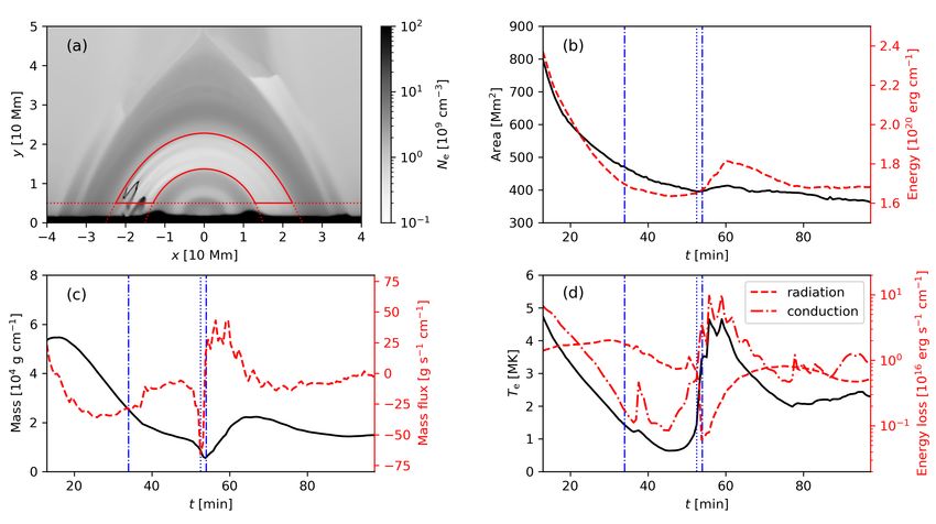
31   of a solar flare event can be divided into three phases: a preflare phase, a sudden, impulsive
32   phase and a gradual or post-flare phase [5]. The magnetic energy is released rapidly in
33   the impulsive phase within a typical timescale of (tens of) minutes. A large fraction of
34   this released energy is transported from the tenuous and hot corona downwards to the
35   denser and colder solar chromosphere via thermal conduction and by energetic electrons
36   [6, 7]. This deposition of energy in the chromosphere leads to a sudden heating of the
37   local plasma, and causes upward evaporation of the plasma to form super hot (∼10 MK)
38   and dense (∼ 1010 cm−3 ) arcade-like loop systems at coronal heights. The loops return
39   to their usual coronal conditions (∼1 MK, ∼ 108 − 109 cm−3 ) in the following, gradual
40   phase, where field-guided thermal conduction and radiative losses generally contribute to
41   the cooling process [8, 9]. These loops, visible in extreme ultraviolet (EUV), but also in
42   Hα images, are usually called post-flare loops (PFLs) [10].
43       Thanks to dramatically increased spatio-temporal resolutions in observations, this grad-
44   ual phase of solar flares is now known to show PFLs which spontaneously develop fine-scale
45   coronal rain [11, 12, 13, 14]. In the multi-thermal coronal rain events, cool and dense rain
46   blobs form in-situ in hot corona, to fall to the chromosphere with speeds up to 100 km s−1 .
47   Coronal rain is also observed in non-flaring coronal loops, is frequently found in loops of
48   active regions [15, 16, 17, 18, 19, 20, 21], and this type of coronal rain has been studied
49   previously using magnetohydrodynamic (MHD) simulations [22, 23, 24, 25, 26]. It has been
50   generally accepted that these rain blobs are generated in a catastrophic cooling process,
51   essentially caused by thermal instability [27, 28, 29, 30]. In a catastrophic cooling event,
52   local temperatures drop from 1 MK to below 0.1 MK within one minute, while local den-
53   sities can increase by orders of magnitude [14]. Observations of flare-driven coronal rain
54   demonstrate that this catastrophic cooling can also happen in PFLs, but this has thus
55   far never been modeled. The actual post-flare coronal rain trigger is yet to be identified:
56   recent work showed that it can not be due to electron beams [31]. Another phenomenon
57   thought to have a close relationship with these sudden condensations are the so-called dark
58   post-flare loops (DPFLs), where some PFL loops suddenly vanish from specific EUV pass-
59   bands, e.g. at 17.1 nm, 30.4 nm and 21.1 nm [32, 33, 34]. In these DPFLs, an EUV loop
60   which was bright for a while suddenly darkens for several minutes, so effectively disappears
61   between the adjacent EUV loops seen at the same height. It has been suggested that the
62   formation of cool and dense coronal rain may contribute to EUV emission and absorption,
63   inducing DPFL formation [33, 34]. However, this suggestion must still be confirmed in an
64   ab-initio model. Besides coronal rains, multi-thermal plasma behaviour is at stake in many
65   setting, e.g. in galactic outflows or in giant molecular clouds in the interstellar medium
66   [35, 36, 37].
67       Here we perform an MHD simulation of a flare event from its pre-flare phase all the
68   way into the gradual phase. This simulation finally allows us to understand the complex
69   thermodynamic evolutions of PFLs. For the first time in any modeling effort, we (1)
70   reproduce post-flare coronal rain; (2) quantify the chromosphere-corona mass and energy
71   cycles during PFLs; and (3) demonstrate the intricate relationship between condensations

                                                   2
72 and the disappearing EUV loops, or DPFLs.
73 Post-flare loop formation and evolution
74 In solar flare events, arcade-like PFLs form in the impulsive phase due to magnetic recon-
75 nection and are filled with hot and dense plasma by evaporation flows from the chromo-
76 sphere. In our two and a half dimensional (2.5D) simulation, we simulate the cross-sectional
77 view on an extended flaring arcade system, with the assumption that plasma parameters
78 do not vary in the direction across the arcade. The simulation plane runs perpendicular to
79 the (evolving) flare ribbons that mark the PFL footpoints. The hot PFL plasma releases
80 soft X-ray (SXR) photons via thermal bremsstrahlung and EUV photons of specific ener-
81 gies due to electron de-excitation, making the PFLs light up in the SXR waveband and
82 at selected EUV wavelengths. Synthesizing our MHD simulation in this early impulsive
83 phase gives mock observational views shown in Fig. 1. Solar flares are classified as A, B,
84 C, M or X level, according to their peak SXR flux in the 1-8 Å waveband measured near
85 Earth. This peak flux in our simulation is about 4×10⁻⁷ W cm−2 when assuming that the
86 loop width in the third direction is 100 Mm (see also Fig. 2e), therefore the simulated flare
87 is a B level flare.
Figure 1: SXR (panel a, emission in 3-6 keV) and EUV image (panel b, at 13.1 nm) of our
simulated flare at its impulsive phase (t = 6 min). The right, 13.1 nm emission has peak
temperatures at 105.6 K and 107 K. Solid lines are magnetic field lines.
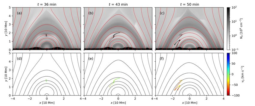
88 Fig. 2 demonstrates the full evolution in magnetic topology, from pre-flare current sheet
89 to the formation of PFLs at the impulsive phase (Fig. 2b), extended to the entire evolution
90 of the PFLs through the gradual phase (Fig. 2c,d). There is a vertical current sheet
91 seperating regions of opposite field directions at the beginning of our simulation (Fig. 2a).
392 Magnetic reconnection inside this current sheet produces closed magnetic arcades below and
93 a flux rope above a reconnection site in the impulsive phase (t ≲ 8 min). A large amount of
94 magnetic energy released by reconnection is conducted to the high density chromosphere
95 and this produces upward evaporation flows. They fill the generated coronal loops with
96 hot plasma (∼10 MK) and increase the plasma number density by one order in the PFLs
97 (Fig. 2b). Thereafter, the flare enters the gradual phase when we have a rapidly decreasing
98 magnetic reconnection speed (t ≳ 8 min). The PFL temperature decreases slowly due
99 to thermal conduction and radiative losses in this gradual phase, but suddenly triggers
100 thermal instability near t ≃ 35 min. The loop density also decreases in this period, but is
101 still much higher than the external coronal density (Fig. 2c).
102 Catastrophic cooling driven by thermal instability condenses local plasma in-situ and
103 leads to high density (close to 1011 cm−3 ) and cold (close to 0.01 MK) structures in the
104 coronal PFLs (Fig. 2d). Fig. 2e shows how the SXR flux reaches its peak value at the
105 impulsive phase, to then gradually decrease as the loop temperature drops. The temporal
106 evolution of the total coronal rain material (i.e. Te < 0.1 MK, Ne > 1010 cm−3 and y > 5
107 Mm) is also illustrated in Fig. 2e. We note that sudden condensations happen in two
108 successive events during the entire simulated period. These are located in different loop
109 systems, with the second rain event appearing at a higher altitude.
110 Once condensations happen within PFLs, the formed cold and dense plasma structures
111 will likely fall down from coronal heights due to gravity and hence appear as observed
112 coronal rain blobs. This is fully reproduced in our simulation as demonstrated in Fig. 3.
113 Cold plasma is formed at a PFL looptop at the beginning of the runaway condensation
114 (Fig. 3a). Thereafter, the cold structure extends to lower and higher loops, meanwhile
115 sliding down to one side (Fig. 3b,c). This falling cold plasma gets accelerated to a speed
116 of ∼100 km s−1 by gravity before it enters the chromosphere (Fig. 3d-f). Such a speed
117 is close to that found in coronal rain observations. Considering an acceleration timescale
118 of 10 minutes, the average acceleration rate is lower than the acceleration of gravity. A
119 detailed analysis of rain blob acceleration process for non-flaring (or quiescent) coronal rain
120 was given in [22].
121 Mass and energy cycles during the gradual phase
122 Here we investigate the mass and energy cycles in our entire 100-minute simulation of the
123 gradual phase and the role of condensations in it. To do so, we track mass and energy
124 budgets into the coronal part (y > 5 Mm) of a loop section in which the first round of
125 condensation happens. This loop section is always bounded by (a) the evolving magnetic
126 field line with a fixed footpoint at x = −25 Mm at our lower y = 0 boundary; and by (b)
127 a similarly evolving field line with footpoint at x = −15 Mm (Fig. 4a). As seen in Fig. 3
128 and Fig. 4a, this region gets emptied during the first round of condensations, as matter
129 collects along the field lines into localized rain blobs. This entire loop system continuously
4Figure 2: (a-d): Plasma number density (background color map) and magnetic field topol-
ogy (in red) at t = 0, 6, 29 and 45 min. (e): Temporal evolution of the integral SXR flux
(black solid line) and of the total coronal rain matter (blue dashed line). The PFLs have
an assumed width of 100 Mm in the invariable z-direction, to calculate the SXR flux. The
times corresponding to the top panels are indicated in panel (e) with vertical dotted red
lines.
5Figure 3: (a-c): Plasma number density at t = 36, 43 and 50 min. (d-f): Vertical y-
component of velocity for the coronal cool plasma (Te < 0.1 MK, Ne > 1010 cm−3 and
y > 5 Mm). The solid lines are magnetic field lines.
130 moves downward as a result of the above reconnection dynamics and the corresponding
131 area of the selected region continuously decreases during the simulation as quantified by
132 the solid line in Fig. 4b. The area-integrated total energy (kinetic, thermal and magnetic
133 combined, dashed line in Fig. 4b), area-integrated mass (solid line in Fig. 4c) and the
134 area-averaged temperature (solid line in Fig. 4d) of this region also continuously decrease
135 before the first condensation (t ≃ 35 min). Plasma which evaporated upwards into the
136 corona in the previous impulsive phase now leaks back to the chromosphere in this period,
137 seen in the downward mass flux (dashed line) in Fig. 4c. The decrease of temperature
138 leads to a decrease of the atmospheric scale height. However, this downwards leakage of
139 coronal plasma is severely reduced when the condensation happens after t ≳ 35 min, since
140 the gas pressure in the coronal part of the loop then decreases rapidly. Therefore, we see
141 a drop of the downward mass flux in Fig. 4c near t ≈ 38 min, when condensations fully
142 formed. Later on, the downward mass flux experiences a sudden increase, exactly when
143 the cool coronal rain material goes through the lower y = 5 Mm boundary of the studied
144 region. The area-integrated mass reaches its minimum value when all cool material leaves
145 and enters the chromosphere. Thereafter, plasma from the chromosphere is injected to the
146 loop again, due to the low pressure inside the loop, leading to an upwards mass flux. The
147 total mass then gradually returns to its value before condensation.
148 The changing coronal energy budget shows a similar tendency with the changing coronal
149 mass cycle. The energy also experiences a decrease in the pre-condensation and during the
6Figure 4: (a): Plasma number density at t = 52 min. The region bounded by the field lines
starting from (x, y) = (−25 Mm, 0) and (x, y) = (−15 Mm, 0) and the horizontal line y =5
Mm is investigated in panels b-d. (b): Time evolution of the evolving area (black solid line)
and that of integrated total energy (red dashed line). (c): Time evolution of integrated
mass (black solid line) and of the mass flux across the lower boundaries of this region.
(d): Time evolution of average temperature (black solid line), integral radiative losses (red
dashed line) and integral conductive losses (red dashed-dotted line). Blue vertical dashed-
dotted lines indicate the starting and ending time of the condensation, and the vertical
blue dotted line marks the time of panel a.
7150 condensation phase, to then experience an increase after the condensations merged into
151 the chromosphere due to renewed plasma injection (Fig. 4b). It has been suggested that
152 thermal conduction determines the PFLs energy loss at the beginning of the gradual phase
153 of a flare and that subsequently radiative losses will become dominant [38]. Our simulation
154 shows that this suggestion is correct before and also during the occurring condensations.
155 The efficiencies of radiative cooling and of thermal conduction to the energy loss in the
156 selected region are compared in Fig. 4d. The contribution of thermal conduction is greater
157 than radiative losses for t ≲ 25 min, but conductive losses drop gradually owing to the
158 decreasing temperature gradient. At t ≈ 25 min, the average temperature is about 3 MK,
159 and the efficiency of radiative losses becomes most prominent. However, conductive losses
160 become stronger than radiative losses again when the condensations vanished from the
161 loop system, as collisions between re-injected flows from both footpoints make the loop hot
162 again and the radiative loss drop for a while due to the decrease of loop density.
163 Catastrophic cooling and rain-induced QPP
164 The first round of condensation happens near t ≈ 35 min. The temporal evolutions of in-
165 stantaneous maximum/minimum temperature/number density in the condensation region
166 (the same as marked in Fig. 4a) are illustrated in Fig. 5. Triggering of thermal instability
167 switches the radiative cooling process from linear to nonlinear, and then leads to a catas-
168 trophic cooling of local plasma. We get an average temperature decreasing rate of -9000
169 K s−1 in the catastrophic cooling phase. In contrast, the cooling rate before catastrophic
170 cooling is -3000 K s−1 . As a result of catastrophic cooling, the local temperature decreases
171 from 0.2 MK to 0.02 MK within half a minute (Fig. 5a), while the local number density
172 increases by one order, from 1010 cm−3 to 1011 cm−3 (Fig. 5b).
173 A quasi-periodic pulsation (QPP) with a period of ∼ 3 minutes appears in the maximum
174 density curve, just after the rain condensation disappeared from the PFL system. This QPP
175 is caused by the injected flows mentioned in the previous section, refilling and reheating
176 the PFL. The density variation due to these flows along a field line is shown in Fig. 4c.
177 Injected flows propagating from one footpoint to the other produce reflected slow mode
178 waves. Such a process has previously been studied in [39] for isolated loop systems. The
179 sharp density changes in Fig. 4c are shocks ahead of the injection flows and the wave fronts
180 of the slow mode waves. Such QPPs hence reflect density variations in the low corona due
181 to flows or wave propagation. The period of our QPP is close to the time for the slow
182 mode wave to propagate from one footpoint to the other, as the wave speed is about 300
183 km s−1 .
8Figure 5: (a): Time evolution of maximum/minimum temperature in the region showing
coronal rain from Fig. 4a. (b): Evolution of maximum/minimum number density in the
same region. (c): Time-space plot of the number density along a field line with y = 0
footpoints at x = ± 24.5 Mm, after the rain left the studied loop region, and a quasi-
periodic oscillation appears. The midpoint of the field lines is at s = 0 and negative s
indicates the left side.
9184 Coronal rain and dark post-flare loops
185 In synthesized EUV images of our simulation, coronal loop(s) appear in the gradual phase.
186 An example is shown in Fig. 6 at the 17.1 nm waveband. Interestingly, this loop disappears
187 for about 10 minutes during the evolution, as demonstrated in panels (a) to (e) of Fig. 6.
188 The sudden darkening of the bright EUV loop in our simulation resembles the dark post-
189 flare loop (DPFL) phenomenon, previously observed at the same 17.1 nm passband and
190 with similar timescale of 10 minutes [32]. Observed DPFLs and the disappearing EUV
191 coronal loop in our simulation also share the same time evolution of integral EUV flux:
192 the EUV flux reaches its minimum value when the darkening happens (compare Fig. 3 in
193 ref. [32] and our Fig. 6f). The formation of a darkened coronal EUV loop needs to satisfy
194 one or both of the following conditions: (1) an emission drop in an existing bright EUV
195 loop; (2) an absorption of the background EUV emission [40]. Here we explain how these
196 conditions can be satisfied based on our simulation results.
Figure 6: (a-e): Time evolution of synthetic EUV 17.1 nm images. The regions in cyan
have temperatures lower than 0.1 MK. (f): Time evolution of the integral EUV 17.1 nm
flux from a region y > 5 Mm. Red vertical dashed lines in panel (f) give the corresponding
times of panels (a-e).
197 The role of cool and dense coronal plasma in EUV emission and absorption leading to
198 DPFLs has been emphasized previously [33, 34], with coronal rain observations [11, 12, 13,
199 14] and our simulation results showing how this cool and dense plasma can be generated in
200 PFLs. The drop in the loop emission is understood from our simulation: loop temperature
201 changes relate to nearby rain condensations. Indeed, the temperature of bright loops in
202 this 17.1 passband (about 105.8 K) is not far from the critical temperature for the onset
10203 of catastrophic cooling (this is density and temperature dependent, but generally happens
204 below 2 MK according to [41]). Condensations can be triggered by thermal instability
205 near bright loops and these suddenly formed structures grow fastest across magnetic field
206 lines (counterintuitive due to the field-aligned thermal conduction, but see [22, 29, 30, 42]).
207 Rain that forms near (Fig. 6a-b), and ultimately inside (Fig. 6c) the bright coronal loops,
208 thus causes the darkening as illustrated in Fig. 6c-d. Once condensation happens, a lot
209 of plasma will collect into a small region, so the plasma density elsewhere in the loop
210 decreases. To maintain pressure balance, these evacuated loop regions will increase in
211 temperature, so EUV brightness decreases due to these combined temperature and density
212 changes. Ultimately, the loop refills and brightens once more (Fig. 6e).
213 Summary
214 To fully understand coronal rain in PFLs and the mass and energy budget in the gradual
215 phase of solar flares, we performed the first flare simulation from onset all the way into the
216 long duration post-flare phase. Post-flare coronal rain successfully and repeatedly forms.
217 The flare-induced rain is a result of catastrophic cooling by thermal instabilities, and our
218 simulation shows successive rain formation at increasing heights in the PFL configuration.
219 Falling rain blobs into the chromosphere lead to sudden mass drops in PFLs, but their
220 mass increases again due to spontaneously forming injection flows. Therefore, the coronal
221 rain events do not accelerate the PFL mass loss in the longer term. Such longer term mass
222 loss is more determined by the change of the gravity scale height due to the cooling of
223 PFLs.
224 Both thermal conduction and radiative losses contribute to the energy budget in PFLs.
225 Thermal conduction dominates the PFL energy loss at the beginning of the gradual phase.
226 Thereafter, it becomes less efficient than radiative losses, owing to decreases in loop tem-
227 perature and in temperature gradient. However, thermal conduction can efficiently recover
228 again after a condensation falls to the chromosphere, as the loop reaches again a high
229 temperature. In this phase, an emptied loop refills and can show a slow-wave related QPP.
230 We showed that the formation of DPFLs can result from post-flare rain condensations.
231 Condensations change loop temperatures and can make existing bright EUV loops tem-
232 porarily disappear for several minutes. This timescale of EUV loop darkening is identical
233 to observed DPFLs.
234 Methods
235 Simulation setup
236 We perform the simulation with the open-source MPI-AMRVAC code [43, 44]. The sim-
237 ulation is 2.5D, where the domain is 2D but all vector quantities have three components.
11238 The simulation domain is given by -75 Mm ≤ x ≤ 75 Mm and 0 ≤ y ≤ 100 Mm. This
239 simulation box has an initial resolution of 96 × 64, but an equivalent high resolution of
240 3072 × 2048 is achieved with our block-adaptive mesh. The governing equations are the
241 magnetohydrodynamic (MHD) equations with effects of gravity, thermal conduction, ra-
242 diative loss and magnetic field dissipation due to resistivity included, also shown in [7]
243 (the source terms related to fast electrons have not been activated here). The new multi-
244 dimensional field-line-based transition region adaptive conduction (TRAC-L) method is
245 adopted to properly handle the chromosphere-corona interaction at affordable resolution
246 [45].
247 A relaxation has been done to obtain a static pre-flare atmosphere before we perform
248 the flare simulation. A background heating is required to offset the energy losses due to
249 radiative cooling and thermal conduction. Inspired by [46], this background heating is a
250 function of initial and spatio-temporally evolving values, given by
( )2
T0 (y)
Hb (x, y, t) = 0.5{tanh[(y − htra )/ha ] + 1}Ne,0 (y)Ne (x, y, t) G(T0 (y)), (1)
T (x, y, t)
251 where htra = 3 Mm, ha = 0.1 Mm, Ne indicates number density, subscript 0 indicates the
252 t = 0 initial value and G(T ) is the radiative cooling curve adopted in our simulations. The
253 cooling curve from [47] is used. The initial vertical temperature T0 (y) profile in [48] (model
254 C7) is employed. The number density at y = 40 Mm is set to 2 × 109 cm−3 and the initial
255 density profile is calculated based on hydrostatic equilibrium. In the relaxation stage, a
256 uniform vertical magnetic field is adopted. A numerically static atmosphere is obtained
257 after a relaxation time corresponding to 3.5 hours. The local number density at y = 40
258 Mm decreases to about 109 cm−3 after this relaxation. The final instantaneous background
259 heating rate of this relaxed stage is saved and then used in the subsequent flare simulation.
260 After the relaxation, the magnetic field configuration is changed. The magnetic config-
261 uration from [46] is employed then, given by
Bx = 0, (2)
−B0 ,
x < −λ
By = B0 , x>λ (3)
B0 sin[πx/(2λ)], else
√
Bz = B02 − By2 , (4)
262 where B0 = 30 G is the new initial magnetic field strength and λ = 10 Mm. Such
263 a configuration allows magnetic reconnection. A three-stage resistivity strategy is then
264 activated. A spatially localized resistivity inside the initial current sheet triggers magnetic
265 reconnection in the first stage. This localized resistivity is given by
{
η1 [2(r/rη )3 − 3(r/rη )2 + 1], r ≤ rη
η(x, y, t < tη1 ) = (5)
0, r > rη
12where η1 = 0.1, r = x2 + (y − hη )2 , hη = 40 Mm, rη = 2.4 Mm and tη1 = 31 s. In the
√
266
267 second stage, we use an anomalous resistivity given by
{
0, vd ≤ vc
η(x, y, tη1 < t < tη2 ) = (6)
min{αη (vd /vc − 1) exp[(y − hη ) /hs ], 1},
2 2 vd > vc
268 where αη = 1 × 10⁻³ , hs = 10 Mm, tη2 = 7.78 min, vd (x, y, t) = J/(eNe ) and vc =
269 128, 000 km s−1 . The resistivity is set to zero in the third stage t > tη2 to force the flare to
270 enter the gradual phase, where only numerical dissipation happens. The resistivity strategy
271 used in our first and second stage is similar to that in [49].
272 We employ symmetric boundary conditions for number density, pressure and magnetic
273 field components, while anti-symmetric conditions are employed for velocity components at
274 the left and right boundaries. At the upper and bottom boundaries, density and pressure
275 are fixed to their initial values. The magnetic field components at the bottom boundary
276 are also fixed to the initial values. An anti-symmetric condition is applied for the x-
277 component of the magnetic field at our upper boundary, while the other two components of
278 the magnetic field employ symmetric conditions there. The velocity at the upper boundary
279 is set to zero. Anti-symmetric conditions are employed for the velocity components at the
280 bottom boundary.
281 The SXR emission is calculated with the method reported in [50]. The EUV emissions
282 are calculated with the contribution function provided by the CHIANTI database and the
283 optically thin assumption [51].
284 Data Availability
285 Simulation data are available on request to W.Z.R. (wenzhi.ruan@kuleuven.be).
286 Code availability
287 The simulation is performed with the open-source AMRVAC code [43, 44], which is available
288 in website http://amrvac.org.
289 References
290 [1] P. A. Sweet, Electromagnetic Phenomena in Cosmical Physics, B. Lehnert, ed. (1958),
291 vol. 6, p. 123.
292 [2] K. Shibata, T. Magara, Living Reviews in Solar Physics 8, 6 (2011).
293 [3] B. Haisch, K. T. Strong, M. Rodono, Ann. Rev. Astron. & Astrophys. 29, 275 (1991).
294 [4] E. M. de Gouveia Dal Pino, P. P. Piovezan, L. H. S. Kadowaki, A&A 518, A5 (2010).
13295 [5] S. R. Kane, Coronal Disturbances, G. A. Newkirk, ed. (1974), vol. 57, p. 105.
296 [6] S. K. Antiochos, P. A. Sturrock, Astrophys. J. 220, 1137 (1978).
297 [7] W. Ruan, C. Xia, R. Keppens, Astrophys. J. 896, 97 (2020).
298 [8] P. J. Cargill, J. T. Mariska, S. K. Antiochos, Astrophys. J. 439, 1034 (1995).
299 [9] M. J. Aschwanden, D. Alexander, Sol. Phys. 204, 91 (2001).
300 [10] A. Bruzek, Astrophys. J. 140, 746 (1964).
301 [11] E. Scullion, L. Rouppe van der Voort, S. Wedemeyer, P. Antolin, Astrophys. J. 797,
302 36 (2014).
303 [12] J.-C. Martínez Oliveros, et al., Astrophys. J. Lett. 780, L28 (2014).
304 [13] J. Jing, et al., Scientific Reports 6, 24319 (2016).
305 [14] E. Scullion, et al., Astrophys. J. 833, 184 (2016).
306 [15] J.-L. Leroy, Sol. Phys. 25, 413 (1972).
307 [16] R. H. Levine, G. L. Withbroe, Sol. Phys. 51, 83 (1977).
308 [17] C. J. Schrijver, Sol. Phys. 198, 325 (2001).
309 [18] E. O’Shea, D. Banerjee, J. G. Doyle, A&A 475, L25 (2007).
310 [19] P. Antolin, L. Rouppe van der Voort, Astrophys. J. 745, 152 (2012).
311 [20] K. Ahn, et al., Sol. Phys. 289, 4117 (2014).
312 [21] P. Antolin, G. Vissers, T. M. D. Pereira, L. Rouppe van der Voort, E. Scullion,
313 Astrophys. J. 806, 81 (2015).
314 [22] X. Fang, C. Xia, R. Keppens, Astrophys. J. Lett. 771, L29 (2013).
315 [23] X. Fang, C. Xia, R. Keppens, T. Van Doorsselaere, Astrophys. J. 807, 142 (2015).
316 [24] S. P. Moschou, R. Keppens, C. Xia, X. Fang, Advances in Space Research 56, 2738
317 (2015).
318 [25] C. Xia, R. Keppens, X. Fang, A&A 603, A42 (2017).
319 [26] P. Kohutova, P. Antolin, A. Popovas, M. Szydlarski, V. H. Hansteen, A&A 639, A20
320 (2020).
321 [27] E. N. Parker, Astrophys. J. 117, 431 (1953).
14322 [28] G. B. Field, Astrophys. J. 142, 531 (1965).
323 [29] N. Claes, R. Keppens, A&A 624, A96 (2019).
324 [30] N. Claes, R. Keppens, C. Xia, A&A 636, A112 (2020).
325 [31] J. W. Reep, P. Antolin, S. J. Bradshaw, Astrophys. J. 890, 100 (2020).
326 [32] Q. Song, J.-S. Wang, X. Feng, X. Zhang, Astrophys. J. 821, 83 (2016).
327 [33] S. Jejčič, L. Kleint, P. Heinzel, Astrophys. J. 867, 134 (2018).
328 [34] P. Heinzel, et al., Astrophys. J. Lett. 896, L35 (2020).
329 [35] W. Banda-Barragán, et al., arXiv e-prints p. arXiv:2011.05240 (2020).
330 [36] R. C. Dannen, D. Proga, T. Waters, S. Dyda, Astrophys. J. Lett. 893, L34 (2020).
331 [37] M. M. Kupilas, C. J. Wareing, J. M. Pittard, S. A. E. G. Falle, Mon. Not. R. Astron.
332 Soc. 501, 3137 (2021).
333 [38] P. J. Cargill, J. A. Klimchuk, Astrophys. J. 605, 911 (2004).
334 [39] X. Fang, D. Yuan, T. Van Doorsselaere, R. Keppens, C. Xia, Astrophys. J. 813, 33
335 (2015).
336 [40] U. Anzer, P. Heinzel, Astrophys. J. 622, 714 (2005).
337 [41] P. J. Cargill, S. J. Bradshaw, Astrophys. J. 772, 40 (2013).
338 [42] Y. H. Zhou, P. F. Chen, J. Hong, C. Fang, Nature Astronomy 4, 994 (2020).
339 [43] C. Xia, J. Teunissen, I. El Mellah, E. Chané, R. Keppens, Astrophys. J. Suppl. 234,
340 30 (2018).
341 [44] R. Keppens, J. Teunissen, C. Xia, O. Porth, Computers & Mathematics With Appli-
342 cations 81, 316 (2021).
343 [45] Y.-H. Zhou, W.-Z. Ruan, C. Xia, R. Keppens, A&A 648, A29 (2021).
344 [46] J. Ye, et al., Astrophys. J. 897, 64 (2020).
345 [47] J. Colgan, et al., Astrophys. J. 689, 585 (2008).
346 [48] E. H. Avrett, R. Loeser, Astrophys. J. Suppl. 175, 229 (2008).
347 [49] T. Yokoyama, K. Shibata, Astrophys. J. 549, 1160 (2001).
348 [50] R. F. Pinto, N. Vilmer, A. S. Brun, A&A 576, A37 (2015).
349 [51] G. Del Zanna, K. P. Dere, P. R. Young, E. Landi, H. E. Mason, A&A 582, A56 (2015).
15350 Acknowledgements
351 This work was supported by the ERC Advanced Grant PROMINENT, an FWO project
352 G0B4521N and a joint FWO-NSFC grant G0E9619N. This project has received funding
353 from the European Research Council (ERC) under the European Union’s Horizon 2020
354 research and innovation programme (grant agreement No. 833251 PROMINENT ERC-
355 ADG 2018). This research is further supported by Internal funds KU Leuven, through the
356 project C14/19/089 TRACESpace. The computational resources and services used in this
357 work were provided by the VSC (Flemish Supercomputer Center), funded by the Research
358 Foundation–Flanders (FWO) and the Flemish Government–department EWI.
359 Author contributions
360 W.Z.R performed the simulation and wrote the first draft. Y.H.Z contributed to the
361 implementation of the TRAC-L method and revision of the paper. R.K initiated the
362 study, supervised the project, led the discussions and contributed to revision of the paper.
363 All authors contributed to discussions.
364 Competing interests
365 The authors declare no competing interests.
16You can also read