A HYDROCHEMICALLY GUIDED LANDSCAPE-BASED CLASSIFICATION FOR WATER QUALITY: A CASE STUDY APPLICATION OF PROCESS-ATTRIBUTE MAPPING (POAM) AT A ...
←
→
Page content transcription
If your browser does not render page correctly, please read the page content below
ESSOAr | https://doi.org/10.1002/essoar.10507536.1 | CC_BY_4.0 | This content has not been peer reviewed.

    A hydrochemically guided landscape-based classification for water quality: a case
       study application of process-attribute mapping (PoAM) at a national scale

Clinton W.F. Rissmann1,2, Lisa K. Pearson1, Adam P. Martin3, Matthew I. Leybourne4, W.
Troy Baisden5, Timothy J. Clough6, Richard W. McDowell7, and Jenny G. Webster-Brown7

1
    Land and Water Science, 90 Layard Street, Invercargill 9810, New Zealand.
2
 Waterways Centre for Freshwater Management, University of Canterbury and Lincoln
University, Private Bag 4800, Christchurch 8140, New Zealand.
3
    GNS Science, Private Bag 1930, Dunedin 9054, New Zealand.
4
 Queen’s Facility for Isotope Research, Department of Geological Sciences and Geological
Engineering, and Arthur B. McDonald Canadian Astroparticle Physics Research Institute,
Department of Physics, Engineering Physics & Astronomy, Queens University, Kingston,
Ontario, Canada.
5
    University of Waikato, Private Bag 3105, Hamilton 3240, New Zealand.
6
    Lincoln University, PO Box 85084, Lincoln 7647, New Zealand.
7
 National Science Challenge, AgResearch, Lincoln Science Centre, Private Bag 4749,
Christchurch 8140, New Zealand.

Corresponding author: Clinton Rissmann (clint@landwatersci.net)

OICID
Clinton Rissmann 0000-0002-1550-5365
Lisa Pearson 0000-0002-0746-871X
Adam Martin 0000-0002-4676-8344
Matthew Leybourne 0000-0002-2361-6014
Troy Baisden 0000-0003-1814-1306
Tim Clough 0000-0002-5978-5274
Richard McDowell 0000-0003-3911-4825
Jenny Webster Brown 0000-0001-9665-871X

Key Points:
      •   A few dominant processes (atmospheric, hydrological, redox, chemical and physical
          weathering) govern spatial variability in water quality
      •   Hydrochemistry is used to guide the mapping of dominant process-gradients and
          expert knowledge and machine learning is used to validate
      •   Failure to consider dominant process-gradients in modeling and policy application risks
          poor water quality outcomes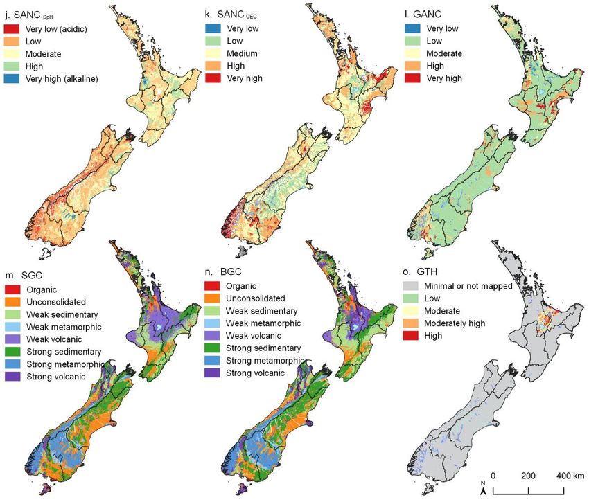
ESSOAr | https://doi.org/10.1002/essoar.10507536.1 | CC_BY_4.0 | This content has not been peer reviewed.

Abstract
Spatial variation in landscape attributes can account for much of the variability in water quality
compared to land use factors. Spatial variability arises from gradients in topographic, edaphic,
and geologic landscape attributes that govern the four dominant processes (atmospheric,
hydrological, microbially mediated redox, physical and chemical weathering) that generate,
store, attenuate, and transport contaminants. This manuscript extends the application of Process
Attribute Mapping (PoAM), a hydrochemically guided landscape classification system for
modelling spatial variation in multiple water quality indices, using New Zealand (268,021 km²)
as an example. Twelve geospatial datasets and >10,000 ground and surface water samples from
2,921 monitoring sites guided the development of 16 process-attribute gradients (PAG) within a
geographic information system. Hydrochemical tracers were used to test the ability of PAG to
replicate each dominant process (cross validated R2 of 0.96 to 0.54). For water quality, land use
intensity was incorporated and the performance of PAG was evaluated using an independent
dataset of 811 long-term surface water quality monitoring sites (R2 values for total nitrogen of
0.90 - 0.71 (median = 0.78), nitrate-nitrite nitrogen 0.83 - 0.71 (0.79), total phosphorus 0.85 -
0.63 (0.73), dissolved reactive phosphorus 0.76 - 0.57 (0.73), turbidity 0.92 - 0.48 (0.69), clarity
0.89 - 0.50 (0.62) and E. coli 0.75 - 0.59 (0.74)). The PAGs retain significant regional variation,
with relative sensitivities related to variable geological and climatic histories. Numerical models
or policies that do not consider landscape variation likely produce outputs or rule frameworks
that may not support improved water quality.

Plain Language Summary
In the wrong place, or at excessive concentrations, nutrients (nitrogen and phosphorus) and
sediment become contaminants. Along with pathogens (harmful microbes), they require
reduction to improve water quality globally. Landscape variation can result in significant
differences in water quality despite similar land use pressures. Landscape variation been mapped
for New Zealand using a novel landscape classification system, termed Process Attribute
Mapping to explain how and why water quality varies spatially. The classification uses twelve
pre-existing map datasets and >10,000 ground and surface water samples from 2,921 monitoring
sites to depict differences as national process attribute gradient (PAG) maps. Each PAG was
tested against tracers (such as chloride, iron, and calcium) measured in surface water samples.
The ability of PAG to represent steady-state water quality, as indicated by nitrogen, phosphorus,
sediment, and a microbial indicator, was assessed by combining an independent dataset of 811
long-term surface water quality monitoring sites and a map representing the gradient in land use
intensity. The modelling identified regional climatic and geological variation as key controls on
water quality variation across New Zealand. The PAG will now be combined into a single
national classification for water quality. This methodology should be applicable globally.

ESSOAr | https://doi.org/10.1002/essoar.10507536.1 | CC_BY_4.0 | This content has not been peer reviewed.

1 Introduction
        Water quality, as indicated by concentrations of nitrogen and phosphorus species, organic
and inorganic sediment, and the faecal indicator bacterium Escherichia coli (E. coli), can vary
spatially across a landscape, even when land use is spatially uniform. These water quality
differences occur because of natural spatial variation in several processes (atmospheric,
hydrological, microbially mediated redox, physical and chemical weathering) that determine the
composition of water (Moldan and Černý, 1994; Clark and Fritz, 1997, Drever and Stillings,
1997; Kendall and McDonnell, 1998; Güler et al., 2002; McMahon and Chapelle, 2008;
Tratnyek et al., 2012; Daughney et al. 2015). These processes are also coupled to gradients in
landscape attributes, such as topography and geology.
         Gradients in the volume and intensity of precipitation, an atmospheric process, are
primarily driven by weather patterns and local scale topographic variation (landscape attribute)
(Clark and Fritz, 1997; Drever and Stillings, 1997; Kendall and McDonnell, 1998). The
hydrological process is driven by climate, catchment topography, edaphic and geological
attributes (Clark and Fritz, 1997; Kendall and McDonnell, 1998; James and Roulet, 2006;
Inamdar, 2011). Groundwater redox depends on the abundance of electron donors within an
aquifer (Drever and Stillings, 1997; Krantz and Powars, 2000; McMahon and Chapelle, 2008).
Mass weathering processes are determined by bedrock characteristics (Mueller and Pitlick,
2013). The pH, ionic composition, and alkalinity of surface and ground waters is strongly
influenced by the acid neutralising capacity of soil and rock (Wright, 1988; Drever and Stillings,
1997; Leybourne and Goodfellow, 2010). These and other component processes may account for
the majority of water quality variation, compared to land use on its own, through regulating the
generation, storage, attenuation, and transport of contaminants in the environment (Johnson et
al., 1997; Hale et al., 2004; King et al., 2005; Dow et al., 2006; Shiels, 2010; Becker et al.,
2014). Accordingly, the role that landscape plays in determining water quality variation is
critically important, and especially so for geologically diverse settings, such as New Zealand
(Johnson et al., 1997).
        Given the importance of landscape attributes, many ‘controlling landscape factor'
classifications have been developed to generate landscape or riverine classes that discriminate
variation in water quality. Such classification schemes include: 1) the United States
Environmental Protection Agency's and the United States Geological Survey's Ecoregion and
Ecological land approaches, which have been applied globally (Dinerstein et al., 2017; Omernik
and Griffith, 2014; Sayre et al., 2014); 2) the European Water Framework Directive's Ecoregions
(Hughes and Larsen, 1988; European Commission, 2000); and 3) the River Environment
Classification, which has been applied across New Zealand (Snelder et al., 2005). These
landscape classification schemes typically employ a top-down approach that groups landscape
attributes into classes according to similar climatic, topographic, edaphic, or geologic attributes,
and these have been used to discriminate variation in a wide range of characteristics, including
hydrology, water quality and ecological characteristics.
       In the work presented here, hydrochemical knowledge, in conjunction with measures of
process-specific tracers in surface and shallow groundwaters, is used to guide the identification,
organisation, and subsequent classification of landscape attributes that govern gradients in each
dominant process. The focus on mapping dominant processes gradients and the use of
hydrochemical tracers to guide the classification of the landscape differs from traditional
landscape factor classification methods (Hughes and Larsen, 1988; Omernik and Griffith, 2014;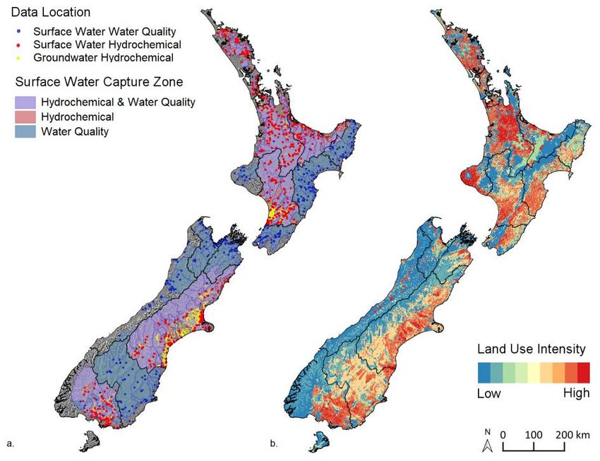
ESSOAr | https://doi.org/10.1002/essoar.10507536.1 | CC_BY_4.0 | This content has not been peer reviewed.

Sayre et al., 2014; Dinerstein et al., 2017). Surface and groundwater chemistry is a valuable tool
for reconstructing the origins and history of water (Clark and Fritz, 1997; Drever, 1997; Kendall
and McDonnell, 1998). Analysing hydrochemical tracers, for a given process, within surface
waters and shallow unconfined aquifers also provides a process-level reference or control point.
This permits relationships between processes and landscape attributes to be evaluated and
hypotheses regarding such relationships to be refined. Thus, hydrochemistry is useful for guiding
the production of a more representative classification than is possible through a purely top-down
approach.
        In addition to the established understanding of the relationship between process gradients
and landscape attributes provided by hydrochemistry, we also hypothesise that a small number of
dominant processes govern spatial variation in water quality. This hypothesis follows Grayson
and Blöschl’s (2001) dominant process concept, which suggests that the response of
environmental systems is generally explained by a small number of dominant processes. Grayson
and Blöschl (2001) also proposed that a logical way to identify the dominant processes is by
evaluating the sensitivity of the system to each of the individual processes (believed to have
influence) through a (high-order) multi-variable sensitivity analysis and selecting those variables
with significant influence (Sivakumar, 2004; 2008).
        This manuscript describes the application and testing of a hydrochemically guided
landscape classification system specifically for water quality. The method, developed originally
for Southland, New Zealand, is termed Process-Attribute Mapping (PoAM) (Rissmann et al.,
2019). PoAM applies a practical hydrochemical method, at a macroscale, to generate spatial
representations of the four dominant processes that determine spatial variation in water quality:
this generates a series of graphical outputs, or maps. Each graphical output is referred to as a
‘process-attribute gradient’ that represents, at a macroscale, the coupling between a dominant
process (or component process) and its controlling landscape attributes.

2 Materials and Methods

       2.1 High level overview of PoAM method
         The PoAM conceptual framework and model presented here was developed from
Rissmann et al. (2018a, 2019; Fig. 1) and a step-by-step description of the PoAM method is
provided in the supporting information S1. Two examples of process-attribute gradient
development are also provided to support the readers understanding of the method (S2 and S3).
Further, examples of the use of hydrochemical and water quality data to generate process-
attribute gradients are provided by Rissmann et al. (2016a, 2018a, b, 2019). The PoAM method
results in a depiction of the landscape, at a macroscale, showing zones within the landscape at a
level where dominant process occur (e.g., redox, not denitrification). Through mapping each
dominant process gradient instead of an individual contaminant (e.g., nitrate only), reaction
process (e.g., denitrification only), or hydrological pathway (e.g., vertical percolation through the
soil matrix to an underlying aquifer only), PoAM produces macroscale, landscape classifications
capable of providing process-level context. For example, 'why' is nitrate concentration elevated
in one stream but not another?
ESSOAr | https://doi.org/10.1002/essoar.10507536.1 | CC_BY_4.0 | This content has not been peer reviewed.

Figure 1. A flow chart summary of key steps in process-attribute mapping (PoAM) (adapted
from Rissmann et al., 2019; see S1). The conceptual model provides a spatial representation of
the key processes and contaminant transport pathways whilst the numerical models provide an
estimate of steady-state median surface water concentration. PAG: process-attribute gradient.

       PoAM utilises existing geospatial classifications of climate, topography, soil, geology
and hydrochemical data to build graphical representations of each process-attribute within a
geographic information system (GIS). During the development of process-attribute gradients,
hydrochemical data is used to:
          i.    refine hypotheses about controlling landscape factors through evaluating the
                relationship between hydrochemical process signals and landscape attributes;
         ii.    support the identification and combination of relevant landscape attributes from
                pre-existing geospatial datasets to generate process-attribute gradients; and
        iii.    drive the grouping of landscape attributes into classes.
        Following process-attribute gradient development, a series of high-level hypotheses are
proposed about the likely sensitivity and magnitude of response (i.e., increase or decrease in
concentration) of each hydrochemical tracer(s) for each dominant process. Each hypothesis is
tested using the hybrid deterministic genetic programming (HDGP) approach of Schmidt and
Lipton (2015). The HDGP method is specifically designed to reveal the underlying relationships
ESSOAr | https://doi.org/10.1002/essoar.10507536.1 | CC_BY_4.0 | This content has not been peer reviewed.
between a target variable (i.e., hydrochemical tracer) and one or more predictors (i.e., process-
attribute gradients). The method employs symbolism (white box), is unsupervised and
evolutionary, discarding any process-attribute gradients that do not reduce the modelled
relationships uncertainty and complexity (Khu et al., 2001; Schmidt and Lipson, 2009, 2015;
Rissmann et al., 2019). The machine defined sensitivities and magnitude of response for each
tracer are compared with the hypothesised response derived from expert knowledge of the
process level controls (Fig. 1; Rissmann et al., 2019). If the machine defined response is
consistent with the hypothesis for each hydrochemical tracer and the modelled relationships are
reasonable, i.e., cross-validated R2 > 0.65, they are considered to provide a representation of the
actual process-attribute gradient. Only then are process-attribute gradients deemed fit to be
combined with a representation of land-use pressure and development of water quality models. If
a region is characterised by a distinct geological feature (e.g., geothermal activity), or climatic
history (e.g., no history of glaciation), deviation from the high-level hypotheses is expected.
In practice, the multivariate testing of process-attribute gradients requires surface water
capture zones to be generated for each surface water hydrochemical site (n = 730 nationally) and
mean scores for each process-attribute gradient to be calculated. Median hydrochemical
concentrations and mean process-attribute scores are then spatially joined in a tabular format and
used as the input for multivariate assessment (Fig. 1). Following multivariate testing of the
hydrochemical tracers of each dominant process, a representation of land use pressure (i.e.,
intensity) is incorporated and process-attribute gradients are used to evaluate spatial variation in
median total nitrogen, nitrate-nitrite nitrogen, total phosphorus, dissolved reactive phosphorus, E.
coli, clarity (black disk), and turbidity (Nephelometric turbidity units) across 811 long-term
surface water quality monitoring sites nationally.
2.2 Case study setting
New Zealand is characterised by a diversity of topography, climate, soil type, geology,
and land cover. The New Zealand climate varies from subtropical in the north to cool temperate
in the south, with cold (< 0 °C mean annual temperature) alpine conditions in the mountainous
areas. Rainfall is typically between 300 and 1600 mm per annum, although this can exceed 9000
mm across alpine regions of the South Island. Relief is up to 3724 m along the north-northeast
trending Southern Alps mountain chain that bisects the South Island (Fig. 2), and isolated
volcanic centres are up to 2797 m-high on the North Island. Andosols and Cambisols (United
Nations, Food and Agricultural Organisation Soil Classification) are the dominant soil types,
with multiple other soil types present, including Podzols, Luvisols, Gleysols, Arenosols,
Acrisols, Panosols, Phaeozems and Nitisols (de Sousa et al., 2020). The geology of New Zealand
is divided into a variety of volcanic, intrusive and sedimentary terranes that make up the
basement rocks of the Austral Superprovince, and the overlying, mainly sedimentary and
volcanic rocks of the Zealandia Megasequence, are separated from basement by a diachronous
regional unconformity between 117 and 105 Ma (Edbrooke et al., 2015). Land cover (updated
2018) is dominated by pasture (c. 40 %), indigenous forests (c. 26 %), cropland, exotic forest and
urban areas. New Zealand has > 70 major river systems and c. 425 000 km-length of rivers and
streams, with 51 % in catchments dominated by native vegetation and the rest in modified
landscapes (Ministry for the Environment and Stats NZ, 2020). High temperature (> 180 C)
volcanic-hydrothermal activity is mainly restricted to the Taupo Volcanic Zone (Fig. 2).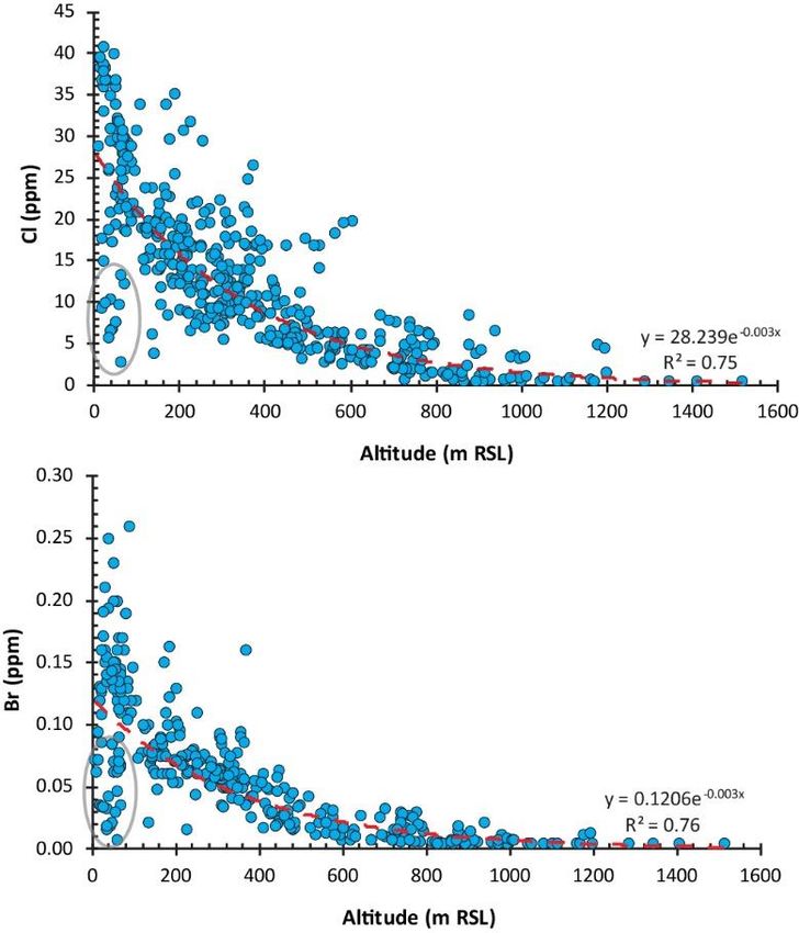
ESSOAr | https://doi.org/10.1002/essoar.10507536.1 | CC_BY_4.0 | This content has not been peer reviewed.

Figure 2. Map of New Zealand subdivided by region. Also shown is the trace of the Southern
Alps mountain chain and the location of the Taupo Volcanic Zone. Base layer is realistic land
cover from Geographx (2009).

3 Data

         3.1 Hydrochemical and water quality datasets
        Chemical analyses of low, median, and event flows were taken from 730 long-term
surface water monitoring sites across the regions of Northland, Auckland, Waikato, Bay of
Plenty, Manawatū-Whanganui, Canterbury, and Southland (58 % of New Zealand), between
2017 and 2019 (Table 1 and Fig. 3). Across the same regions and for the same time period, data
for the sample chemical constituents were collected at 2,191 long-term groundwater monitoring
sites (Table 1). The respective hydrochemical datasets for surface water and groundwater were
subsequently combined with pre-existing hydrochemical data collected between 2007-2017 and
median concentrations calculated (Pearson and Rissmann, 2021a). Detailed information of the
sampling methodologies, field measures, laboratory analysis, calculation of hydrochemical
metrics (e.g., major ion facies, saturation indices) and quality assurance and quality control of the
samples used in this project are provided in Rissmann et al. (2016).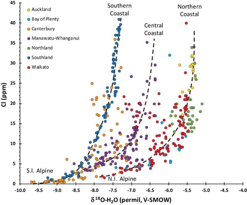
ESSOAr | https://doi.org/10.1002/essoar.10507536.1 | CC_BY_4.0 | This content has not been peer reviewed.
Table 1. Hydrochemical and water quality analyses used in this study.
Dataset Type Analyte Units Parameter Name
Hydrochemical Major Ca mg/L Dissolved calcium 1
(surface water Constituents Cl mg/L Dissolved chloride
and
groundwater) DOC mg/L Dissolved organic carbon
HCO3 mg CaCO3/L Dissolved bicarbonate alkalinity 2
K mg/L Dissolved potassium
Mg mg/L Dissolved magnesium
Na mg/L Dissolved sodium
SO4 mg/L Dissolved sulphate
SiO2 mg/L Dissolved reactive silica
Minor B mg/L Dissolved boron
Constituents Br mg/L Dissolved bromide
F mg/L Dissolved fluoride
Fe mg/L Dissolved iron
I mg/L Dissolved iodide
Mn mg/L Dissolved manganese
Field Clarity m Visual clarity
Parameters DOField mg/L Dissolved oxygen (field measured)
EC µS/cm Electrical conductivity 3, temperature corrected
ORP mV Oxidation-reduction potential
pHField pH units pH (field measured)
pHLab pH units pH (lab measured)
Temp C Water Temperature
Water quality Nutrients TN mg N/L Total nitrogen
(surface water) NNN mg N/L Nitrate nitrite nitrogen
TP mg P/L Total phosphorus
DRP mg P/L Dissolved reactive phosphorus
Suspended Black disk m Visual clarity
Sediment
Turb NTU4 Turbidity
Biological E. coli cfu/100 mL Escherichia coli
1 Mostsamples were filtered (0.45 µm) prior to analysis, and therefore analytical results reflect “dissolved” rather than total
concentrations. However, it is noted that many colloidal species will pass through a 0.45 µm filter.
2 The United States Geological Survey notes that alkalinity is not a chemical in water, but, rather, it is a property of water that is
dependent on the presence of bicarbonates, carbonates, and hydroxides. As such, alkalinity is defined as a measure of the ability
of the water body to neutralize acids and bases and thus maintain a fairly stable pH level.
3 Microsiemens
per centimeter.
4 Nephelometric turbidity units.
An independent surface water quality dataset comprising 991 long-term monitoring sites
across New Zealand was downloaded from Land Air Water Aotearoa (LAWA) for 2014 – 2018
(Table 1 and Fig. 3a). This dataset was collected by each regional authority, with quality
assurance performed according to National Environmental Monitoring and Reporting Standards
(Davies-Colley et al., 2012). A minimum of 60 repeat measures are included for each site.
Internal quality control in this project removed urban catchments and sites with point source
impacts, including sites downstream of municipal wastewater discharges, reducing the dataset to
811 sites. Site water quality medians were calculated for each monitoring point (Pearson and
Rissmann, 2021b). No water quality measures from the 811 long-term monitoring sites were
used in the generation of process-attribute gradients.
ESSOAr | https://doi.org/10.1002/essoar.10507536.1 | CC_BY_4.0 | This content has not been peer reviewed.
Figure 3. a) Surface and ground water sample locations for hydrochemical (Table 1) and water
quality data sets (Table 2 – a minimum of 60 repeat samples for each site) used in PoAM; and b)
A map of the land use intensity gradient across New Zealand. The regional boundaries are shown
by black outlines.
3.2 Geospatial datasets
For the national application of PoAM, attributes were selected from several national and
one regional GIS datasets. This included: 1) topography, elevation and altitude from an 8 m
digital elevation model (Land Information New Zealand, 2012); 2) geological attributes from the
1:250 000 geological map series (QMAP, Heron, 2014) and the New Zealand Land Resource
Inventory (NZLRI; 1:50 000; Manaaki Whenua Landcare Research, 2000a,b; Newsome et al.,
2008; Lynn et al. 2009); 3) soil attributes from SMap (1:50 000, Manaaki Whenua Landcare
Research, 2019a) and Fundamental Soils Layer (1:50 000; Manaaki Whenua Landcare Research,
2000c); 4) land cover from the Land Cover Database (LCDBv5; Manaaki Whenua Landcare
Research, 2019b); and 5) land use from Land Use Mapping Report (LUCASv006; Ministry for
the Environment, 2019). For hydrological input data: 1) river lines, stream Strahler order and
catchment areas (capture zones) were sourced from the River Environment Classification (v 2.4;
Snelder and Biggs, 2002); 2) precipitation volume was derived from the National Climate
Database (Ministry for the Environment, 2016); 3) 18O-H2O of precipitation came from the
national isoscape model of Baisden et al. (2016); 4) water table depth is from Westerhoff et al.
(2018); and 5) geothermal extent is from Bibby et al. (1995) for the Taupo Volcanic Zone (Fig.
2).
Land use intensity and land use for microbial contaminants were derived by combining
the Land Use Capability classification of Lynn et al. (2009), LCDBv5 land cover (Manaaki
Whenua Landcare Research, 2019b) and LUCAS land use (Ministry for the Environment, 2019)
and ranking land use intensity from 1ow to high using expert judgement (Fig. 3b).
ESSOAr | https://doi.org/10.1002/essoar.10507536.1 | CC_BY_4.0 | This content has not been peer reviewed.
3.3 Process-attribute gradient generation
After quality assurance, hydrochemical and geospatial datasets were used to generate 16
national-scale process-attribute gradients depicting the four dominant processes (Tables 2, Fig.
1). A high-level summary of the hypotheses and process-attribute gradients are included in
Supporting Information 1. Examples of the assessment and development of the precipitation
source 18O-H2O (V-SMOW) and geological reduction potential process-attribute gradients are
provided in Supporting Information 2 and 3, with further detail of the process-attribute
gradients developed provided in Pearson (2015a, b) and Rissmann et al. (2016a, 2018a).
During process-attribute gradient development, a series of high-level hypotheses were
developed linking the likely sensitivity and magnitude of the response of individual process-
attribute gradients to one or more tracers of each dominant process (see S1). For example, based
on observed relationships between process signals in water and landscape attributes, a hypothesis
was formulated that the conservative tracers of water source, e.g., Cl and Br, will exhibit a
positive magnitude (concentration increases) across the macroscale recharge domain from
(lowest) Alpine to Hill to Lowland (highest). This hypothesis is consistent with the role of
altitude and distance from the coast over the rainout of marine aerosols, an orographic
atmospheric process (Clark and Fritz, 1997; Nichol et al., 1997; Rissmann et al., 2016a; see S1
and S2). Hypothesis development included recognising that two or more dominant processes and
multiple process-attribute gradients may be required to adequately explain the spatial distribution
of one or more hydrochemical tracers across the surface water network (Rissmann et al., 2019).
If a region is characterised by a distinct geological (e.g., geothermal activity), or climatic history
(e.g., no history of glaciation), variation in the process-attribute gradients retained is expected.
When used for generating water quality models, overland flow, soil slaking and
dispersion process-attribute gradients were normalised by the area of developed land (i.e., non-
native land cover). This normalization is based on evidence of contaminant source limitation,
i.e., low/no anthropogenic contaminant loads, across large areas of undeveloped hill and high
country where overland flow is highest, in contrast to developed land with similar topography.
The normalisation of these two process-attribute gradients within water quality model
development defines a process response resulting in a negative magnitude for most water quality
measures, or a sink, for undeveloped land and positive magnitude of these measures for
developed land.
A regional-scale geothermal process-attribute gradient was also developed using the
apparent resistivity (log of apparent resistivity m) model of Bibby et al. (1995); there is
evidence for diffuse geothermal inputs, from high enthalpy (≥ 180 °C) volcanic-hydrothermal
systems, influencing hydrochemical composition and water quality of the Bay of Plenty and
Waikato regions.ESSOAr | https://doi.org/10.1002/essoar.10507536.1 | CC_BY_4.0 | This content has not been peer reviewed.
Table 2. Summary of the 16 national-scale process-attribute gradients. Relevant datasets and
their scale are also shown.
Process PAG Process attribute Relevant datasets and scales Attributes
gradient
Atmospheric O18 Precipitation source 8 m DEM, δ18O-H2O precipitation δ18O-H2O, altitude, distance from the
isoscape (4 km2 pixel) coast
PPT Precipitation volume Annual average rainfall (5 km2 pixel) Precipitation volume
Hydrological RCD Macroscale recharge Soil surveys (1:50,000), Aquifer type Altitude, temperature isotherm, river
domain and extent (1:50,000) network, Typic
Udifluvent (Fluvial Recent) soils
OLF Overland flow Soil surveys (1:50,000), 8 m DEM Soil texture, drainage class,
permeability, slope, area of developed
land
DD Deep drainage Soil surveys (1:50,000) Drainage class, permeability, depth to
slowly permeable horizon
LAT Lateral drainage Soil surveys (1:50,000) Drainage class, permeability, depth to
slowly permeable horizon,
ART Artificial drainage Soil surveys, 8 m DEM, Land Cover (1 Drainage class, permeability, depth to
ha) slowly permeable horizon, slope,
agricultural land cover
HYD Soil slaking and Soil surveys (1:50,000) Soil texture, drainage class,
dispersion as a soil permeability, area of developed land
hydrological index
NBP Soil zone bypass Soil surveys (1:50,000) Cation exchange capacity, pH
EWT Equilibrium water table Water Table Model (0.04 km2 pixel) Modelled water table depth
and aquifer potential
Redox SRP Soil reduction potential Soil surveys (1:50,000); soil chemistry Drainage class, carbon content
profile points.
GRP Geological aquifer Geological surveys (1:50,000 - Rock type (main and sub rocks)
reduction potential 1:250,000)
Weathering SANC Soil acid neutralization Soil surveys (1:50,000); geochemical Soil pH, cation exchange capacity
capacity baseline survey (8 km2)
GANC Geological acid Geological surveys (1:50,000 - Rock type
neutralization capacity 1:250,000); geochemical baseline
survey (8 km2)
SGC Surface/top regolith Geological surveys (1:50,000 - Rock type and strength
strength 1:250,000)
BGC Basal regolith strength Geological surveys (1:50,000 - Rock type and strength
1:250,000)
Geothermal GTH High enthalpy Log of resistivity (limited to extent of Resistivity
geothermal (≥180 °C) Taupo Volcanic Zone, Fig.1)
PAG: process attribute-gradient; DEM: digital elevation model
4 Multivariate Assessment
4.1 Pre-processing of data
Following process-attribute gradient production, mean surface water capture zone
process-attribute scores were calculated for the 730 regional hydrochemical and 811 national
water quality monitoring sites (Fig. 1). Mean land use intensity scores and capture zone area (ha)
were calculated for each capture zone. Mean capture zone scores were joined with the
hydrochemical and 5-year water quality datasets. A constant was added to all numeric data to
remove 0 or negative values, and the dataset log10 transformed prior to multivariate assessment.
4.2 Hypotheses testing and evaluation of the representativeness of process-attribute
gradients
Multivariate testing was first applied to the hydrochemical dataset (Step 4, Fig. 1; see
S1). In this analysis, tracers of each dominant process are the target variables, and process-
attribute gradients the predictors. The multivariate assessment provides an independent test ofESSOAr | https://doi.org/10.1002/essoar.10507536.1 | CC_BY_4.0 | This content has not been peer reviewed.
the sensitivity (importance) and magnitude of response (increase or decrease in concentration) of
process-attribute gradients relative to specific hydrochemical tracers of each dominant process
(i.e., atmospheric, hydrological, redox, and weathering). This step is important for evaluating the
validity of the high-level hypotheses generated during process-attribute gradient development
(see Table S1.1 and S1.2). For example, the performance of the process-attribute gradients in
replicating water source and hydrological connectivity is evaluated against the conservative
hydrological tracers Cl and Br; the representativeness of the redox process-attribute gradients is
evaluated against FeII and dissolved organic carbon (DOC), and so on. The hydrochemical
tracers are chosen based on their relevance as an indicator for a given process. Tracers that have
a significant land use origin, e.g., nitrogen, phosphorus or E.coli are not used to test process-
attribute gradients. For example, dissolved FeII, not total, is used as a redox tracer because of its
role as a terminal electron acceptor during microbially mediated redox succession. Iron is also
the 5th most abundant element in Earth’s crust so is rarely source-limited (Hem, 1985). However,
evaluating physical weathering process-attribute gradients is limited by the lack of suitable
geochemical tracers, with simple proxies such as clarity and turbidity, a poor substitute for multi-
element or isotope proxies of sediment source. Testing of process-attribute gradients was
undertaken on the combined data set for the seven regions and repeated with focus on regional
subsets due to evidence for geographically independent process level controls over water quality
(e.g., geothermal activity).
4.3 Water quality models
Given the evidence for geographically independent process-level controls (e.g.,
geothermal activity), water quality models were run as regional subsets characterised by similar
climatic and geological histories.
5 Results
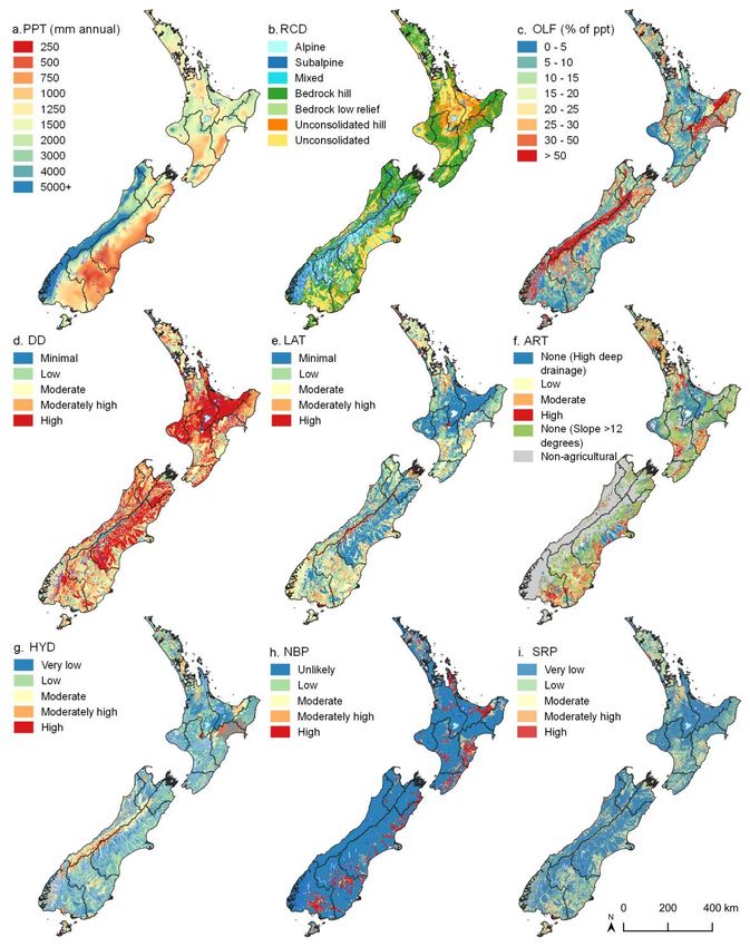
5.1 Process-attribute gradients
Sixteen process-attribute gradients defining the dominant processes governing
hydrochemistry were produced nationally (Fig. 4, S2 and S3). Of the 16 process-attribute
gradients, two are associated with atmospheric drivers prior to the routing of water by the
hydrological network and are macroscale; precipitation volume (Fig 4a) and 18O-H2O of
precipitation (V-SMOW; see S2). Eight process-attribute gradients are associated with the
hydrological drivers of spatial variation in hydrochemistry. Of these, the recharge domain and
hydrological connectivity layer are macroscale (Fig. 4b). The remaining seven hydrological
process-attribute gradients are all associated with the soil zone and represent mesoscale
hydrological gradients in percent precipitation occurring as overland flow, deep drainage through
the soil profile, lateral drainage, artificial drainage of the soil profile, soil slaking and dispersion,
shrink-swell mediated soil zone bypass (Fig 4c-h) and water table depth and aquifer potential
(see S3). The two redox (Fig 4i, S3) and both chemical and physical weathering processes (5
process-attribute gradients) are comprised of separate soil and geological process-attribute
gradients (Fig. 4j-n). Soil process-attribute gradients overlie geological process-attribute
gradients, except where bedrock outcrops (Rissmann et al., 2019). Across lowland areas, the
geological process-attribute gradients represent the upper portion of the unconfined aquifer
system (Rissmann et al., 2019). The regional-scale geothermal process-attribute gradient
represents high enthalpy ( 180 C) diffuse volcanic-hydrothermal inputs over theESSOAr | https://doi.org/10.1002/essoar.10507536.1 | CC_BY_4.0 | This content has not been peer reviewed. hydrochemistry and water quality (i.e., ammoniacal N and P) of shallow ground and surface water across the Taupo Volcanic Zone (Fig. 4o). Combined, these layers provide the user with a conceptual, macroscale understanding of the landscape factors known to influence water quality across New Zealand. Figure 4. Examples of process attribute gradients representing the 4 dominant processes. a) atmospheric process showing precipitation volume, b) hydrological process showing recharge domain, c) overland flow, d) deep drainage, e) lateral drainage, f) artificial drainage, g) soil
ESSOAr | https://doi.org/10.1002/essoar.10507536.1 | CC_BY_4.0 | This content has not been peer reviewed.

hydrological index of slaking and dispersion, h) natural soil zone bypass under soil moisture
deficit, i) redox process showing soil reduction potential.

Figure 4 continued. Examples of process attribute gradients representing the 4 dominant
processes. j) weathering (chemical) showing soil acid neutralizing capacity by pH, k) soil acid
neutralizing capacity by cation exchange capacity, l) geological acid neutralizing capacity, m)
weathering (physical) showing surface lithology and rock strength, n) basal lithology and rock
strength, and o) geothermal process showing resistivity for the Taupo Volcanic Zone. Acronyms
are defined in Table 2.

       5.2 Hypothesis testing and representativeness evaluation
       The performance of PoAM to replicate the effective atmospheric, hydrological, redox,
and weathering gradients across the seven regions is presented in Table 3. Machine-defined
functions for the dominant processes responded as hypothesised, and except for clarity (R2 0.52),
cross-validated R2 values of 0.61 to 0.84 indicate moderate to very good representation of macro-
and mesoscale hydrological gradients and mesoscale redox and chemical weathering gradients
(Table 3).
ESSOAr | https://doi.org/10.1002/essoar.10507536.1 | CC_BY_4.0 | This content has not been peer reviewed.
Table 3. Cross-validated performance of process-attribute gradients to estimate hydrochemical
tracers of each dominant process across 7-regions.
Correlation Maximum Mean Squared Mean Absolute
Process Tracer R2 Complexity
Coefficient Error Error Error
Cl 0.69 0.83 1.98 0.24 0.36 57
Hydrology
Br 0.70 0.83 1.89 0.21 0.32 78
K 0.73 0.86 1.99 0.20 0.30 72
FeII 0.61 0.79 2.78 0.32 0.36 31
Redox
DOC 0.80 0.90 2.53 0.25 0.33 26
Total Alkalinity 0.71 0.84 2.07 0.28 0.39 35
Chemical
Ca 0.67 0.82 2.55 0.25 0.35 33
Weathering
SiO2(aq) 0.84 0.92 1.87 0.19 0.32 59
Physical
Clarity 0.76 0.88 1.67 0.15 0.23 48
Weathering
DOC: dissolved organic carbon
As expected, performance at the regional subset-scale was significantly better than at the
national-scale for all tracers (Table 3 and 4). The process-attribute gradients defined and
retained, and their relative sensitivities, are presented for each regional subset in Supporting
Information 4. At a high-level, macroscale precipitation source (O18), precipitation volume and
recharge domain were retained as the most sensitive predictors of the conservative hydrological
tracers Cl and Br; soil reduction potential, soil drainage class equivalents and geological
reduction potential were retained as the most sensitive predictors of the redox tracers FeII and
DOC, and; soil and geological acid neutralisation capacity were retained as the most sensitive
predictors of total alkalinity, Ca and dissolved reactive silica (SiO2(aq)). As we hypothesised, the
atmospheric and hydrological process-attribute gradients were retained alongside redox and
chemical weathering tracers as sensitive predictors of observed spatial variation. The retention of
atmospheric and hydrological process-attribute gradients reflects the important role of water
source, precipitation volume and macroscale routing of water over spatial variation in redox and
weathering process signals. Although machine-defined functions for each dominant process
responded as hypothesised, significant variation in the process-attribute gradients retained and
their relative sensitivities were observed between regional subsets (see S4).ESSOAr | https://doi.org/10.1002/essoar.10507536.1 | CC_BY_4.0 | This content has not been peer reviewed.
Table 4. Model performance for hydrochemical tracers of dominant processes across regional
subsets.
Tracer Regional Subset R2 Correlation Maximum Mean Mean Complexity
Coefficient Error Squared Absolute
Error Error
Cl Northland - Auckland 0.82 0.91 0.77 0.04 0.13 45
Waikato - Bay of Plenty 0.71 0.85 1.74 0.14 0.24 41
Manawatu 0.84 0.92 0.87 0.06 0.18 47
Canterbury 0.79 0.89 1.87 0.18 0.26 53
Southland 0.95 0.98 0.74 0.05 0.16 22
Br Northland - Auckland 0.74 0.87 0.94 0.16 0.31 66
Waikato - Bay of Plenty . . . . . .
Manawatu 0.78 0.88 1.93 0.11 0.19 38
Canterbury 0.71 0.85 1.92 0.25 0.34 74
Southland 0.87 0.93 1.65 0.13 0.19 37
K Northland - Auckland 0.79 0.89 0.82 0.06 0.17 30
Waikato - Bay of Plenty 0.84 0.92 1.82 0.17 0.26 36
Manawatu 0.77 0.88 1.61 0.12 0.19 42
Canterbury 0.86 0.86 0.86 0.86 0.86 50
Southland 0.80 0.90 1.17 0.05 0.14 34
FeII Northland - Auckland 0.71 0.85 3.37 0.39 0.33 58
Waikato - Bay of Plenty 0.95 0.97 0.48 0.03 0.13 57
Manawatu 0.79 0.90 0.20 0.01 0.05 53
Canterbury 0.56 0.80 2.35 0.17 0.19 44
Southland 0.87 0.93 1.65 0.11 0.23 37
DOC Northland - Auckland 0.74 0.87 1.72 0.10 0.17 57
Waikato - Bay of Plenty . . . . . .
Manawatu 0.82 0.91 1.12 0.07 0.16 40
Canterbury 0.54 0.74 2.09 0.18 0.25 42
Southland 0.96 0.98 0.98 0.06 0.16 38
Total Northland - Auckland 0.66 0.82 1.41 0.23 0.34 45
Alkalinity Waikato - Bay of Plenty 0.81 0.90 1.09 0.09 0.22 51
Manawatu 0.75 0.87 2.55 0.33 0.36 48
Canterbury 0.78 0.88 1.45 0.18 0.32 27
Southland 0.92 0.96 0.80 0.06 0.17 47
Ca Northland - Auckland 0.71 0.86 1.64 0.15 0.25 44
Waikato - Bay of Plenty 0.75 0.87 1.58 0.13 0.24 34
Manawatu 0.88 0.94 1.05 0.11 0.23 47
Canterbury 0.75 0.87 2.76 0.30 0.36 72
Southland 0.93 0.96 0.91 0.06 0.16 38
SiO2(aq) Northland - Auckland 0.62 0.79 1.07 0.11 0.22 38
Waikato - Bay of Plenty 0.86 0.96 0.84 0.09 0.20 38
Manawatu 0.80 0.90 0.86 0.08 0.18 43
Canterbury 0.78 0.89 1.06 0.07 0.17 42
Southland 0.78 0.89 0.84 0.05 0.16 37
Clarity Northland - Auckland 0.93 0.96 0.11 0.00 0.03 31
Waikato - Bay of Plenty 0.67 0.82 0.48 0.02 0.11 27
Manawatu 0.72 0.86 0.41 0.02 0.10 78
Canterbury 0.52 0.72 0.63 0.05 0.16 48
Southland 0.82 0.91 0.59 0.01 0.08 31ESSOAr | https://doi.org/10.1002/essoar.10507536.1 | CC_BY_4.0 | This content has not been peer reviewed.
5.3 Performance of process-attribute gradients to predict water quality
The observed sensitivities and associated magnitude of response of process-attribute
gradients supported the high-level hypotheses, so land-use gradients (Fig. 3b) were incorporated,
and water quality models were developed for each regional subset. Median cross-validated
performance measures were calculated from regional subsets and are summarized in Table 5.
Median performance measures include a cross-validated R2 of 0.78 for total nitrogen, 0.79 for
nitrate-nitrite nitrogen, 0.73 for total phosphorus, 0.73 for dissolved reactive phosphorus, 0.69
for turbidity (Nephelometric turbidity units), 0.62 for clarity (black disk), and 0.74 for E. coli.
The regional subset performance measures are presented in Table 6 and retained process-
attribute gradients and sensitivities provided in Supporting Information 5.
Table 5. Median cross-validated performance measures for 811 water quality sites nationally.
TN NNN TP DRP Turb. Clarity E. coli
R2 0.78 0.79 0.73 0.73 0.69 0.62 0.74
Correlation coefficient 0.89 0.89 0.85 0.86 0.83 0.79 0.87
Maximum error 0.59 0.85 0.65 0.58 0.74 0.55 0.90
Mean squared error 0.03 0.10 0.03 0.04 0.05 0.02 0.07
Mean absolute error 0.13 0.21 0.11 0.12 0.15 0.11 0.19
Complexity 33 42 38 38 42 35 35
DRP: Dissolved Reactive Phosphorus; E. Coli: bacterial indicator; NNN: Nitrate-Nitrite Nitrogen; TN: Total Nitrogen; TP: Total
Phosphorus; Turb.: Turbidity in Nephelometric Units.
In terms of sensitivity, the gradients retained for each water quality measure and each
regional subset were, overall, consistent with expert knowledge. For example, artificial drainage
and soil reduction potential process-attribute gradients were amongst the most sensitive
predictors of nitrate-nitrite nitrogen (negative magnitude), total phosphorus, and dissolved
reactive phosphorus (positive magnitude) across regional subsets; regolith cohesion status
process-attribute gradients were amongst the most sensitive predictors of total phosphorus,
dissolved reactive phosphorus (positive magnitudes), clarity (negative magnitude) and, to a
lesser degree, turbidity (positive magnitude). Artificial drainage and natural bypass (cracking
soils) were amongst the most sensitive predictors of E. coli (positive magnitudes). Normalized
by the area of developed land, overland flow exhibited a positive magnitude for most water
quality measures. Overall, land-use intensity process-attribute gradients were retained as the
most sensitive predictors of total nitrogen and nitrate-nitrite nitrogen and E. coli (positive
magnitudes) but were less commonly retained and of lower sensitivity for total phosphorus,
dissolved reactive phosphorus, turbidity (NTU), and clarity. However, regional subsets showed
significant variation in performance measures and process-attribute gradients retained by the
statistical model.ESSOAr | https://doi.org/10.1002/essoar.10507536.1 | CC_BY_4.0 | This content has not been peer reviewed.
Table 6. The cross-validated performance measures for 811 water quality sites by regional
subset.
Analyte Regional Subset R2 Correlation Maximum Mean Mean Complexity
Coefficient Error Squared Absolute
Error Error
TN Northland - Auckland 0.90 0.95 0.38 0.01 0.06 33
Waikato - Bay of Plenty 0.81 0.90 0.79 0.03 0.12 39
Wellington-Manawatu-Taranaki 0.78 0.89 0.57 0.03 0.13 19
Hawkes Bay - Gisborne 0.74 0.87 0.73 0.04 0.13 23
West Coast-Tasman-Nelson 0.75 0.87 0.59 0.04 0.14 86
Marlborough-Canterbury 0.71 0.85 0.71 0.10 0.24 17
Southland - Otago 0.86 0.93 0.54 0.03 0.12 41
NNN Northland - Auckland 0.83 0.92 0.78 0.06 0.15 23
Waikato - Bay of Plenty 0.82 0.91 0.67 0.05 0.16 43
Wellington-Manawatu-Taranaki 0.81 0.90 0.83 0.05 0.17 25
Hawkes Bay - Gisborne 0.73 0.86 0.99 0.10 0.21 29
West Coast-Tasman-Nelson 0.79 0.89 1.02 0.10 0.21 44
Marlborough-Canterbury 0.71 0.84 1.75 0.21 0.31 42
Southland - Otago 0.79 0.89 0.85 0.11 0.25 42
TP Northland - Auckland 0.83 0.92 0.38 0.02 0.08 30
Waikato - Bay of Plenty 0.72 0.85 0.74 0.04 0.14 45
Wellington-Manawatu-Taranaki 0.69 0.84 0.53 0.02 0.11 34
Hawkes Bay - Gisborne 0.79 0.89 0.68 0.03 0.11 37
West Coast-Tasman-Nelson 0.73 0.85 0.41 0.03 0.12 43
Marlborough-Canterbury 0.63 0.80 0.65 0.05 0.16 29
Southland - Otago 0.85 0.92 0.65 0.03 0.11 40
DRP Northland - Auckland 0.66 0.85 0.58 0.04 0.11 16
Waikato - Bay of Plenty 0.68 0.82 0.73 0.06 0.19 38
Wellington-Manawatu-Taranaki 0.57 0.77 0.01 0.00 0.00 49
Hawkes Bay - Gisborne 0.75 0.87 0.85 0.04 0.14 35
West Coast-Tasman-Nelson 0.73 0.86 0.50 0.03 0.12 41
Marlborough-Canterbury 0.74 0.86 0.60 0.06 0.19 35
Southland - Otago 0.76 0.88 0.51 0.03 0.12 45
Turbidity Northland - Auckland 0.92 0.96 0.20 0.01 0.05 33
(NTU) Waikato - Bay of Plenty 0.69 0.83 0.85 0.05 0.15 58
Wellington-Manawatu-Taranaki 0.66 0.81 0.76 0.05 0.15 26
Hawkes Bay - Gisborne 0.59 0.78 0.45 0.03 0.11 45
West Coast-Tasman-Nelson 0.74 0.86 0.74 0.06 0.17 66
Marlborough-Canterbury 0.48 0.70 0.90 0.09 0.23 42
Southland - Otago 0.81 0.90 0.54 0.03 0.11 40
Clarity Northland - Auckland 0.89 0.94 0.18 0.00 0.04 33
(Black Waikato - Bay of Plenty 0.73 0.85 0.49 0.02 0.10 37
Disk)
Wellington-Manawatu-Taranaki 0.66 0.82 0.47 0.02 0.11 35
Hawkes Bay - Gisborne 0.61 0.78 0.40 0.02 0.09 40
West Coast-Tasman-Nelson 0.62 0.79 0.55 0.04 0.14 29
Marlborough-Canterbury 0.50 0.72 0.64 0.05 0.16 43
Southland - Otago 0.58 0.77 0.66 0.04 0.12 29
E. coli Northland - Auckland 0.74 0.87 0.39 0.02 0.09 42
Waikato - Bay of Plenty 0.75 0.87 0.90 0.07 0.19 29
Wellington-Manawatu-Taranaki 0.73 0.85 0.77 0.06 0.18 25
Hawkes Bay - Gisborne 0.74 0.86 0.82 0.06 0.17 31
West Coast-Tasman-Nelson 0.59 0.78 1.70 0.14 0.24 52
Marlborough-Canterbury 0.74 0.87 1.24 0.11 0.25 39
Southland - Otago 0.74 0.87 0.90 0.07 0.19 35
DRP: Dissolved Reactive Phosphorus; E.coli: bacterial indicator; NNN: Nitrate-Nitrite Nitrogen; TN: Total Nitrogen; TP: Total
Phosphorus; Turb.: Turbidity in Nephelometric Units.ESSOAr | https://doi.org/10.1002/essoar.10507536.1 | CC_BY_4.0 | This content has not been peer reviewed.
6 Discussion
6.1 The importance of localized geological and climatic histories over water composition
Due to New Zealand's geological diversity, it is unsurprising that the sensitivities of
process-attribute gradients varied between regional subsets. For example, the geothermal
process-attribute gradient was identified as the most sensitive predictor of SiO2(aq) across the
Taupo Volcanic Zone which includes large areas of the Waikato and Bay of Plenty Regions (see
S4). The geothermal process-attribute was also retained as a sensitive predictor of total carbonate
alkalinity. The importance of the geothermal process-attribute gradient over SiO2(aq) and total
alkalinity is consistent with the high partial pressures of CO2 and dissolved silica within the
hydrothermal fluids of the Taupo Volcanic Zone (Giggenbach, 1995). These fluids ascend and
mix with the shallow meteoric aquifers and discharge via the surface water network. Outside the
areas of high enthalpy geothermal activity, the majority of New Zealand soil and geological acid
neutralizing capacity and regolith cohesion process-attribute gradients were retained as the most
sensitive predictors of total alkalinity and dissolved reactive silica.
For water quality, annualized loads of total nitrogen and total phosphorus from the
surface water network to 12 Bay of Plenty region lakes had geothermal contributions up to 29.5
and 68%, respectively (Donovan and Donovan, 2003). This reflects high concentrations of
ammonium and phosphorus in hydrothermal fluids (Hamill, 2018; Giggenbach, 1995). As this
assessment did not evaluate direct inputs of geothermal fluids from the lakebed, these estimates
are likely conservative (see Hamill, 2018). Therefore, it is perhaps unsurprising that the
geothermal process-attribute layer was retained as the most sensitive predictor of total nitrogen
and dissolved reactive phosphorus (positive magnitudes) across both geothermally active regions
within the Taupo Volcanic Zone (see S5). However, land use intensity was retained as the most
sensitive predictor of nitrate-nitrite-nitrogen, probably because of the low redox potential of
geothermal fluids, favoring ammoniacal nitrogen.
In another example, Northland and Auckland were the only regions for which the regolith
cohesion status was retained as the most sensitive predictor of surface water turbidity (NTU) and
clarity (see S5). Here, the regolith cohesion process-attribute gradient is ranked from low to high,
with a negative magnitude of response recorded for turbidity and a positive magnitude of
response for clarity, i.e., turbidity decreases, and clarity increases, as the cohesion status of the
regolith increases. These regions are characterised as the oldest and most weathered in New
Zealand, with no evidence of glaciation, widespread ash fall deposits or significant Quaternary
tectonic activity (Richardson et al., 2013, 2014; Hayward, 2017). The antiquity of the landscape,
an abundance of relatively unconsolidated sedimentary rocks relative to elsewhere in New
Zealand, and Northland's subtropical climate have resulted in high rates of mass wasting and
erosion in response to anthropogenic activity (Richardson et al., 2013, 2014; Swales et al., 2015;
McDonald et al., 2020). Outside of Northland and Auckland, across the much larger area of
geomorphically young landforms, macroscale precipitation source and volume, recharge domain
and hydrological routing, mesoscale hydrological pathway (also of developed land), and both
soil and geological acid neutralization capacity process-attribute gradients are more common
predictors of turbidity and clarity (see S5). The retention of acid neutralization process-attribute
gradients as sensitive predictors of turbidity and clarity is thought to reflect the association
between weak calcareous mudstones and evidence in satellite imagery for higher mass-wasting
rates (Rissmann et al., 2020a).ESSOAr | https://doi.org/10.1002/essoar.10507536.1 | CC_BY_4.0 | This content has not been peer reviewed.
In one final example, Northland-Auckland and Southland-Otago regions contain the
greatest proportion of imperfectly to poorly drained soils (for land < 12° slope) and the highest
concentration of artificially drained (mole-pipe and ditch drainage) agricultural land nationally.
Where artificial drainage is associated with reducing soil profile forms (e.g., gleysols or organic
carbon dominated), redox conditions may enhance phosphorus mobility and associated export to
surface waters (Scalenghe et al., 2010). An abundance of fine-textured and poorly permeable
soils and shallow water tables also favors overland flow. Parsimoniously then, the artificial
drainage density process-attribute gradient was retained as the most sensitive predictor of total
and dissolved reactive phosphorus (positive magnitudes) across these two regional subsets (see
S5). Those regional subsets with a smaller proportion of artificially drained soils retained water
table, soil, and geological reduction potential as sensitive predictors of phosphorus loss.
In summary, differences in the geological and climatic evolution of a region can result in
critical, regional-scale variability in water quality drivers. This variability may be lost when
aggregating data for national models. For example, aggregating the hydrochemistry dataset from
all regions into one model run, the key regional drivers of variation in the process signatures
noted above were lost, and predictive uncertainty increased (Table 3 versus Table 4).
6.2 PoAM performance
Multivariate evaluation shows that process-attribute gradients effectively replicated the
dominant process gradients responsible for the generation, storage, attenuation, and transport of
water quality contaminants in the environment. The observation that spatial variation in water
composition can be reliably estimated as a function of landscape attributes is consistent with
New Zealand and international studies (Johnson et al., 1997; Hale et al., 2004; Snelder and
Biggs, 2002; Snelder et al., 2005; King et al., 2005; Dow et al., 2006; Becker et al., 2014;
Rissmann et al., 2019).
Nonetheless, the identification of regional variations in process-attributes, and their
relative sensitivities, are significant and represent regional-scale variability in geological and
climatic histories. We consider it logical that regions with unique geological attributes or
climatic histories (e.g., high-temperature geothermal activity, deeply weathered regolith, or a
greater abundance of imperfectly to poorly drained soils) will respond differently to land-use
pressures and/or have distinct endogenous sources of water quality contaminants. Our
interpretation is consistent with observed regional variation in the type and severity of water
quality issues across New Zealand (Ministry for the Environment & Stats NZ, 2020).
Overall, the validity and observed performance of the PoAM approach is supported by
the dominant process concept proposed by Grayson and Blöschl (2001), namely:
i. that the response of environmental systems is commonly well explained by the
representation of a small number of dominant processes.
ii. that a logical way to identify the dominant processes governing a system is by
evaluating the sensitivity of the system to each of the individual processes
(believed to have influence) through a (high-order) multi-variable sensitivity
analysis and selecting those variables that are found to have a 'noticeably'
significant influence (Sivakumar, 2004; 2008).ESSOAr | https://doi.org/10.1002/essoar.10507536.1 | CC_BY_4.0 | This content has not been peer reviewed.
6.3 Limitations to Process-Attribute Mapping (PoAM)
Based on expert knowledge and machine defined relationships, process-attribute
gradients provide a reasonable approximation of the macroscale process gradients that govern the
generation, storage, attenuation, and transport of water quality contaminants. However, as with
any complex system, the ability to isolate and depict first-order drivers of process response is
challenging. Accordingly, as with any model each process-attribute layer can only be considered
an approximation of the ‘real’ macroscale process-attribute gradient.
In addition to the challenges of isolating first-order drivers of process response, spatial
correlation between landscape attributes may interfere with the machine-driven isolation of
primary drivers (Rissmann et al., 2019). This is especially true of process-attribute gradients that
share similar landscape attributes. For example, both artificial drainage and soil redox potential
include soil drainage class as one of the controlling landscape attributes. As a result, these two
process-attribute gradients are spatially correlated (R = 0.36) despite representing different
dominant processes, i.e., hydrological versus redox. In some settings, this may result in the
artificial drainage layer being retained as an important predictor of redox sensitive species such
as FeII and DOC. Although dissolved iron and DOC are commonly elevated in mole-pipe
drainage from poorly drained soils (Rissmann and Beyer, 2016), it is incorrect to say that
artificial drainage is a driver of low soil redox potential. In these situations, expert knowledge is
an important basis for interpreting machine defined relationships.
Collinearity is also partially addressed during the evaluation of the sensitivity and
magnitude of response of process-attribute gradients over a given hydrochemical tracer (Fig. 1,
Step 4). Specifically, the HDGP method models each, possibly coupled, variable separately,
intelligently perturbing and destabilising the system to extract its less observable characteristics
and automatically simplifying the equations during modelling (Schmidt and Lipson, 2009, 2015).
This feature of HDGP supports the identification of the most sensitive predictors or closest
approximations of the actual process-attribute gradients governing a given hydrochemical tracer
or water quality measure.
Besides revealing the hidden patterns underlying complex non-linear systems, our
preference for HDGP relates to the important challenge of feature selection in high-dimensional
data sets. For example, we note that Random Forests might overlook important variables.
Specifically, the work of Stijven et al. (2011) noted that although Random Forests can efficiently
find important variables, it may struggle to do so where many variables are equally important.
Poor discrimination of variables with similar weightings results in the sensitivity of predictors
varying randomly, given that such variables are not recognised as being truly distinct. Stijven et
al. (2011) also noted that variable importance is influenced by data distribution, which can result
in misinterpretation and concluded that caution is advised when using Random Forests to decide
which variables to retain, even if the dataset is known not to exhibit strong correlations or
unevenly balanced data. This is because data points in leaf nodes are similar in the nearest
neighbour sense, and the variables selected by Random Forests express proximity. In
comparison, HDGP more robustly identifies important variables if models of sufficient quality
are found (Stijven et al., 2011; Icke and Bongard, 2013; Arnaldo et al., 2014; Schmidt and
Lipson, 2009, 2015).
Another important feature of the machine defined sensitivity analysis employed here
includes the development of a mathematically transparent model (i.e., “white box”) of theYou can also read