Ambient conditions prevailing during hail events in central Europe
←
→
Page content transcription
If your browser does not render page correctly, please read the page content below
Nat. Hazards Earth Syst. Sci., 20, 1867–1887, 2020
https://doi.org/10.5194/nhess-20-1867-2020
© Author(s) 2020. This work is distributed under
the Creative Commons Attribution 4.0 License.

Ambient conditions prevailing during hail events in central Europe
Michael Kunz1,2 , Jan Wandel1 , Elody Fluck1,a , Sven Baumstark1,b , Susanna Mohr1,2 , and Sebastian Schemm3
1 Institute of Meteorology and Climate Research (IMK), Karlsruhe Institute of Technology (KIT), Karlsruhe, Germany
2 Center  for Disaster Management and Risk Reduction Technology, Karlsruhe Institute of Technology (KIT),
Karlsruhe, Germany
3 Institute for Atmospheric and Climate Science, ETH Zürich, Zurich, Switzerland
a now at: Department of Earth and Planetary Sciences, Weizmann Institute of Science, Rehovot, Israel
b now at: Heine + Jud, Stuttgart, Germany

Correspondence: Michael Kunz (michael.kunz@kit.edu)

Received: 13 December 2019 – Discussion started: 2 January 2020
Revised: 5 May 2020 – Accepted: 2 June 2020 – Published: 1 July 2020

Abstract. Around 26 000 severe convective storm tracks be-        recent major loss events include the two supercells on 27–
tween 2005 and 2014 have been estimated from 2D radar             28 July 2013 related to the depression Andreas with eco-
reflectivity for parts of Europe, including Germany, France,      nomic losses of EUR 3.6 billion mainly due to large hail
Belgium, and Luxembourg. This event set was further com-          (Kunz et al., 2018) or storm clusters during Ela on 8–
bined with eyewitness reports, environmental conditions, and      10 July 2014 with economic losses of EUR 2.6 billion (Swis-
synoptic-scale fronts based on the ERA-Interim (ECMWF             sRe, 2015) caused by both large hail and severe wind gusts
Reanalysis) reanalysis. Our analyses reveal that on average       (Mathias et al., 2017). Given the major damage associated
about a quarter of all severe thunderstorms in the investiga-     with SCSs, particularly due to large hail, there is a consider-
tion area were associated with a front. Over complex terrains,    able and increasing need to better understand the local proba-
such as in southern Germany, the proportion of frontal con-       bility of SCSs, their intensity, and their relation to prevailing
vective storms is around 10 %–15 %, while over flat terrain       atmospheric precursors.
half of the events require a front to trigger convection.            Several authors have attempted to establish relations be-
   Frontal storm tracks associated with hail on average pro-      tween SCSs and hailstorms and favorable atmospheric en-
duce larger hailstones and have a longer track. These events      vironments (for Europe: Manzato, 2005; Groenemeijer and
usually develop in a high-shear environment. Using compos-        van Delden, 2007; Kunz, 2007; Sánchez et al., 2009, 2017;
ites of environmental conditions centered around the hail-        Mohr and Kunz, 2013; Púčik et al., 2015; Madonna et al.,
storm tracks, we found that dynamical proxies such as deep-       2018, among others). Hail-conductive environments have
layer shear or storm-relative helicity become important when      been estimated either from proximity soundings or from
separating hail diameters and, in particular, their lengths; 0–   model or reanalysis data, both available over several decades
3 km helicity as a dynamical proxy performs better compared       and, depending on the spatial resolution, on a regional, con-
to wind shear for the separation. In contrast, thermodynam-       tinental, or global scale. According to Púčik et al. (2015),
ical proxies such as the lifted index or lapse rate show only     for example, large hail with a diameter of at least 2 cm most
small differences between the different intensity classes.        likely forms in environments with high values of increasing
                                                                  convective available energy (CAPE) and bulk wind shear.
                                                                  While the former is directly related to the intensity of the
                                                                  updraft, the latter is decisive for the organization’s form of
1   Introduction                                                  the convective systems – single cells, multicells, supercells,
                                                                  and mesoscale convective systems (MCSs; Markowski and
Severe convective storms (SCSs) are responsible for almost        Richardson, 2010). In addition, several studies have sug-
one-third of the total damage by natural hazards in Ger-          gested that SCSs preferentially occur during specific weather
many and central Europe (MunichRe, 2020). Examples of

Published by Copernicus Publications on behalf of the European Geosciences Union.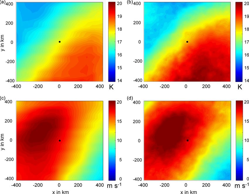
1868                                                                  M. Kunz et al.: Ambient conditions during hail events

regimes, such as European or Scandinavian blocking or tele-        ter. The combination of these reports with storm tracks esti-
connection patterns (Aran et al., 2011; García-Ortega et al.,      mated from radar observations allows us to reconstruct entire
2011; Kapsch et al., 2012; Piper et al., 2019; Mohr et al.,        footprints of SCSs and/or hailstorms.
2019). However, to date, no study has investigated environ-           In our study, we have reconstructed SCS tracks from 2D
mental conditions according to hailstone size and hail swath       radar reflectivity using a cell-tracking algorithm during a
(envelope encompassing all hail streaks; footprint), despite       10-year period (2005–2014) over central Europe including
their relevance to overall storm damage.                           France, Germany, Belgium, and Luxembourg. As our focus
   Forecast experience has shown that synoptic fronts, par-        in on SCSs, we considered only tracks above a reflectivity
ticularly cold fronts during the summer months, can signifi-       of Z ≥ 55 dBZ, a threshold frequently used as hail criterion
cantly modify the convective environment, primarily due to         (e.g., Holleman et al., 2000; Hohl et al., 2002; Kunz and
increasing convective available energy (CAPE) and decreas-         Kugel, 2015; Puskeiler et al., 2016). In order to include ad-
ing convective inhibition (CIN) in combination with cross-         ditional information on the maximum hail diameter of the
frontal circulations leading to lifting and enhanced vertical      SCSs, a subsample of hailstorms (HSs) was created by com-
wind shear. By combining hailstorm tracks determined from          bining the radar-derived SCS tracks with ESWD hail reports.
radar data over Switzerland between 2002 and 2013 with                Afterward, we investigate characteristics and environmen-
front detections (Schemm et al., 2015) based on the Consor-        tal conditions at the time and location of the events unfolding
tium for Small-Scale Modeling (COSMO) analysis, Schemm             for different classes of hail diameter, track lengths (lifetime),
et al. (2016) found that up to 45 % of storms in northeastern      and the relationship with synoptic-scale fronts. Environmen-
and southern Switzerland were associated with a cold front.        tal conditions are assessed by constructing composites of me-
They concluded that mainly wind-sheared environments cre-          teorological fields from the ERA-Interim (ECMWF Reanaly-
ated by the fronts provide favorable conditions for hailstorms     sis) reanalysis centered around the location of a single storm.
in the absence of topographic forcing.                             To estimate the effects of subgrid-scale spatial variations on
   Difficulties in analyzing environmental conditions prior to     environmental conditions, for example, by disturbances in-
or during hailstorms usually arise from insufficient direct hail   duced by orographic features or by temperature and moisture
observations that may serve as the ground truth. The num-          advection, we additionally used the coastDat-3 (set of consis-
ber of ground weather stations is too small to reliably de-        tent ocean and atmospheric data) reanalysis with a resolution
tect all SCSs. High-density hailpad networks exist in only a       about 6 times higher compared to ERA-Interim.
few regions across Europe (e.g., Merino et al., 2014; Her-            The main scientific questions of our study are the follow-
mida et al., 2015) and therefore cannot be used to reproduce       ing:
entire hailstorm footprints. In order to compensate for this
monitoring gap, remote sensing instruments, such as satel-           – How frequent are SCSs associated with a front?
lites (Bedka, 2011; Punge et al., 2017; Ni et al., 2017; Mroz        – Do the characteristics of SCSs associated with a synop-
et al., 2017), lightning (Chronis et al., 2015; Wapler, 2017),         tic cold front differ from those without a front?
or radars (Holleman et al., 2000; Puskeiler et al., 2016; Nisi
et al., 2018), due to their area-wide observability, are used        – How do the environmental conditions in terms of ther-
to estimate the frequency and intensity of SCSs. In particu-           modynamical and dynamical parameters differ between
lar, weather radars can give some indications of hail occur-           hail diameter classes, track lengths, and frontal and non-
rence using either radar reflectivity above a certain threshold        frontal events?
(e.g., Mason, 1971; Hohl et al., 2002) or at specific elevations
in combination with different height specifications (melting         – How does a higher model resolution affect the environ-
level, − 20 ◦ C environmental temperature, and top of the              mental conditions around the SCSs?
storm cell; Waldvogel et al., 1979; Smart and Alberty, 1985;          The paper is structured as follows: Sect. 2 introduces the
Witt et al., 1998). While observations by dual-polarization        datasets and methods used. Section 3 deals with the fre-
radars offer better predictions for hail (e.g., Heinselman and     quency of SCSs and HSs, and Sect. 4 examines the role
Ryzhkov, 2006; Ryzhkov et al., 2013; Ryzhkov and Zrnic,            of synoptic cold fronts and convective storms. Section 5
2019) these systems have been installed in Europe only re-         statistically investigates environmental conditions prevailing
cently and cannot be used for climatological studies.              around the storms for different classes of hail size and track
   Another important data source for hail is severe-weather        length. Section 6 synthesizes and summarizes the major find-
reports from trained storm spotters or eyewitnesses that are       ings, while the most important conclusions are drawn in
pooled into severe-weather archives such as the European           Sect. 7.
Severe Weather Database (ESWD; Dotzek et al., 2009). Al-
though reporting is selective and biased towards population
density and available spotters, these reports provide valuable
information about the intensity of the various convective phe-
nomena associated with SCSs such as maximum hail diame-

Nat. Hazards Earth Syst. Sci., 20, 1867–1887, 2020                                 https://doi.org/10.5194/nhess-20-1867-2020
M. Kunz et al.: Ambient conditions during hail events                                                                       1869

2     Data and methods                                            produced by dynamically downscaling ERA-Interim using
                                                                  COSMO in climate mode (CCLM; Rockel et al., 2008).
The investigation area is central Europe, including Germany,         Mesoscale environments of the hailstorm tracks are char-
France, Belgium, and Luxembourg, from 2005 to 2014,               acterized by severe-storm predictors representing both ther-
where data were available. Since SCSs and HSs in Europe           modynamical and dynamical conditions. We tested and ap-
occur mainly in the summer half-year (SHY; Berthet et al.,        plied several convection-related parameters but focus here
2011; Punge and Kunz, 2016; Púčik et al., 2019), all analy-      only on those proxies with the highest prediction skill: sur-
ses refer to the period from April to September.                  face lifted index (SLI) representing latent instability (Gal-
                                                                  way, 1956), lapse rate (LR) as the temperature difference
2.1    ESWD hail reports                                          between 700 and 500 hPa representing potential instability
                                                                  (only for coastDat-3), deep-layer shear (DLS) as the differ-
                                                                  ence of the wind vectors between 500 hPa and the surface,
The ESWD, managed and maintained by the European Se-              and 0–3 km storm-relative helicity (SRH) quantified by
vere Storms Laboratory (ESSL), is the only multinational
database and by far the largest archive of hail reports in Eu-
                                                                           Z
rope. Quality-checked reports of SCSs and related phenom-         SRH = (v h − c) · (∇ × v h ) dz,                          (1)
ena originate from storm chasers and trained spotters, some-               Z
                                                                                            ∂v

                                                                                                          ∂u
times supplemented by newspaper reports. In our study, we               =      − (u − cx )      + v − cy           dz,      (2)
                                                                                            ∂z               ∂z
consider the reported maximum hail diameters of all qual-
ity levels (70.4 % of all reports were confirmed; 29.0 % were     where v h = (u, v) is the horizontal wind vector and c = (cx ,
at least plausibility checked). This includes both large hail     cy ) is the (constant) cell motion vector, which is usually
with a diameter of at least 2 cm usually given in increments      estimated from a semi-empirical relation such as that from
of 1 cm (in rare cases of 0.5 cm) and hail layers with a depth    Bunkers et al. (2000). As the convective cell-tracking algo-
of at least 10 cm, regardless of hail diameter. In those cases,   rithm directly computes c for each SCS or HS event (see next
and when a hail size is not specified (usually in the case of     Sect. 2.4), we used these values to quantify SRH in addition
small hail), the diameter is set to 1 cm.                         to the vertical wind shear provided by ERA-Interim. Helic-
   During the 10-year investigation period, a total of 4577 re-   ity is a measure of the degree to which the direction of mo-
ports of severe hail in the study area are available. Most        tion is aligned with the (horizontal) vorticity of the environ-
reports stem from Germany (76.5 %), followed by France            ment ωh = ∇ × v h (Markowski and Richardson, 2010). Only
(21.1 %), Belgium (1.7 %), and Luxembourg (0.7 %). This           streamwise vorticity, which is a prerequisite for supercells
distribution does not reflect the occurrence probability of       bearing the largest hailstones, contributes to SRH (Thomp-
SCSs but is primarily due to the ESSL originally being a Ger-     son et al., 2007).
man initiative.
   Because of the large spatial extent of the study area in       2.3   Cold-front detection
a west–east direction, we converted the timestamps for the
daily cycle analysis (only for that; cf. Fig. 2) from UTC into    Synoptic-scale cold fronts are detected in ERA-Interim based
local time (LT) by adding 1t = 24 h/360◦ lat = 4 min per de-      on the method outlined in Schemm et al. (2015), which is
gree starting from 0◦ lat.                                        briefly summarized here. To identify and locate fronts in the
                                                                  reanalysis, we used the thermal front parameter (TFP; Re-
2.2    Reanalyses                                                 nard and Clarke, 1965; Hewson, 1998) defined as
                                                                                      ∇θe
Atmospheric conditions prevailing over a larger area around       TFP = −∇|∇θe | ·          ,                                 (3)
                                                                                     |∇θe |
the SCS tracks are studied using the ERA-Interim (Dee et al.,
2011) reanalysis from the European Center for Medium-             where θe denotes the equivalent potential temperature at
Range Forecast (ECMWF). This dataset, which was also              850 hPa, a widely used choice in the forecasting commu-
used for the detection of synoptic cold fronts (see Sect. 2.3),   nity, which also neglects sea-breeze fronts. The first term in
is represented as spherical harmonics at a T255 spectral reso-    Eq. (3) represents the gradient of the frontal zone (|∇θe |),
lution (approx. 80 km) on 60 vertical levels from the surface     which must be higher than 4 K (100 km)−1 . The second term
up to 0.1 hPa with a temporal resolution of 6 h. In order to      is the unit vector of the θe gradient. The TFP hence captures
estimate the effects of the model resolution on the dynamic       changes of the gradient of the frontal zone along the gradient
and thermodynamic environmental conditions, we addition-          itself. The frontal zone is strongest where TFP = 0, and its
ally used high-resolution coastDat-3 reanalysis data for se-      leading edge is where TFP = max. For the detection of propa-
lected variables. This second reanalysis from the Helmholtz-      gating synoptic fronts, which are in the focus here because of
Zentrum Geestacht (HZG) has a spatial and temporal resolu-        their relevance for convection triggering, we require all fronts
tion of 0.11◦ (approx. 10 km) and 1 h, respectively. It was       to have a length of at least 500 km and a minimum advection

https://doi.org/10.5194/nhess-20-1867-2020                               Nat. Hazards Earth Syst. Sci., 20, 1867–1887, 2020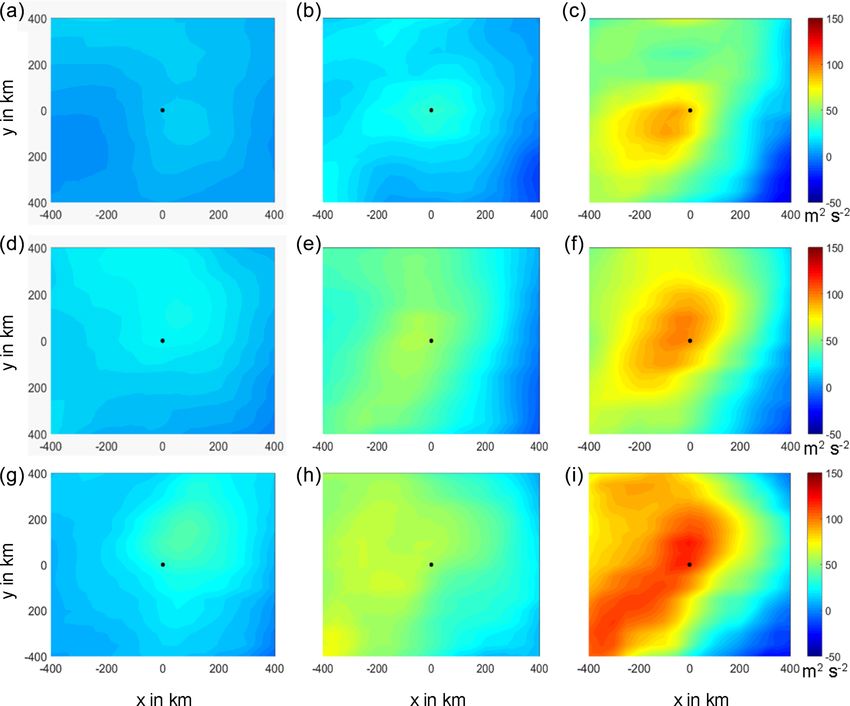
1870                                                                    M. Kunz et al.: Ambient conditions during hail events

speed of 3 m s−1 . These two thresholds may seem somewhat         criterion for hail detection. Several studies have provided ev-
artificial or arbitrary. But as shown by Schemm et al. (2015),    idence that this lower threshold is suitable to identify hail
their implementation sufficiently removes the land–sea con-       in radar data (e.g., Holleman et al., 2000; Hohl et al., 2002;
trast and thermal boundaries from Alpine pumping from the         Kunz and Kugel, 2015; Puskeiler et al., 2016). However,
dataset and limit the data to fronts typically associated with    high radar reflectivity does not guarantee that there is hail on
extratropical cyclones.                                           the ground, mainly because of potential melting hailstones
                                                                  and the relation Z ∼ D 6 , where D is the hail size diameter.
2.4    Radar data and storm tracking                              For example, the evaluation of radar-derived cell tracks with
                                                                  damage data from two insurance companies by Puskeiler
Tracks of SCSs are identified from 2D radar reflectivity          et al. (2016) has shown that the Mason (1971) criterion pro-
based on the precipitation scan at low elevation angles. Radar    vides a satisfactory probability of detection (62 % and 55 %)
data with a spatial and temporal resolution of 1 km and 5 min,    but also a high false-alarm rate (35 % and 40 %). This means
respectively, were provided by Météo France and by the            that our SCS sample based on this criterion consists mainly
German Weather Service (DWD) as entire radar compos-              of hailstorms but also includes some heavy-rain events (see
ites. Whereas all 17 German radars operate in the C band,         Sect. 2.5.2 for the definition of the HS sample).
19 radars in France are in the C band, and 5 each are in             Each SCS event, defined as an entire track reconstructed
the S band and X band. The area in France covered by the          by the tracking algorithm, contains the following parameters:
S-band radars is rather small (< 5 % of the total area) com-      center (latitude and longitude) of the track including date and
pared to that captured by the C band, and these are mainly        time, mean angle, width, total length, and duration; the latter
restricted to the southwest (S-band radars at Opoul, Nîmes,       two quantities allow us to compute the storm motion vec-
Bollène, and Collobrières). Because of the dominance of C-        tors c required for SRH (cf. Eq. 1). For further details on the
band radars, we did not distinguish between the two radar         tracking and the results, see the study by Fluck (2017).
types. X-band radars, exclusively operating in the Maritime
Alps in southeastern France, are not considered due to their      2.5     Combination of SCS tracks with other parameters
strong attenuation of the radar signal.
   Storm tracks were reconstructed by applying a modified         2.5.1    Combination of SCSs with fronts
version of the cell-tracking algorithm TRACE3D originally
                                                                  To match the SCS tracks with synoptic front detections
designed for 3D reflectivity in spherical coordinates (Handw-
                                                                  (cf. Sect. 2.3), we first compute the minimum horizontal dis-
erker, 2002). Thus, TRACE3D has to be modified to rely on
                                                                  tance di between the two events:
2D radar reflectivity in Cartesian coordinates (Fluck, 2017).           q
The tracking algorithm first identifies all convective cells      di = (ai · cos(lat · 2π/360) · l)2 + (bi · l)2 ,          (4)
(reflectivity core; RC) embedded into larger “regions of in-
tense precipitation” (ROIP; Handwerker, 2002). Afterward,         where ai is the longitudinal distance between a frontal grid
the weighted center (barycenter) of all RCs is tracked spa-       point i and the grid points of an individual storm track, bi is
tially over subsequent time intervals dt by establishing a tem-   the same for the latitude, “lat” is the position (latitude) of
poral connection between the detected RCs. For each RC, a         the storm track, and l is the (constant) distance of 1◦ lati-
2D shift velocity vector v T is calculated in different ways,     tude (≈ 111.32 km). The cos function in the equation takes
depending on whether and over what distance an RC has al-         into account the poleward convergence of the lines of longi-
ready been detected in previous scans. The new position of        tude. For each front detection, we compute the distance di
the RC is estimated from s T = v T · δt within a certain search   to all grid points defining the track of an SCS identified in
radius r, which depends on the length of s T and the distance     the same 6 h period. The minimum of all di values, thus
to the closest neighboring RC. This process is repeated for all   dmin = min(di ), defines the minimum distance between the
subsequent scans until the complete track of a convective cell    front and the related SCS.
is reconstructed. The algorithm considers different processes        Frontal SCSs are defined as those events where a front is
such as cell splitting or merging. Correction algorithms are      located within a search radius of R = L/2+200 km (L is the
implemented for undesired radar effects such as the bright        length of an SCS track) around the storm track, i.e., when
band or anomalous propagation (so-called anaprop). In ad-         di < R. Assuming a front acts as a potential trigger for con-
dition, we eliminated all single grid points with high radar      vection, the distance between the two events must be limited
reflectivity but without lightning within a radius of 10 km.      (Trapp, 2013). For this reason and because of the low tem-
This filter is based on the assumption that SCSs are always       poral and spatial resolution of the front detections, we set the
accompanied by lightning. Note that the filter only eliminates    constant part of R to 200 km. Note that changing this part
single spurious signals but keeps the tracks that are composed    to a value of 300 or 400 km has no significant effect on the
of numerous radar grid points.                                    results. The constant part in R (L/2) considers only the time
   In our analyses, we considered only storm tracks above         of the center of the SCSs for the synchronization between the
a threshold of Z ≥ 55 dBZ, referred to as the Mason (1971)        two events. The longer L value is, the larger the temporal and

Nat. Hazards Earth Syst. Sci., 20, 1867–1887, 2020                                https://doi.org/10.5194/nhess-20-1867-2020
M. Kunz et al.: Ambient conditions during hail events                                                                         1871

spatial difference between tracks and fronts can be and, thus,     posites have already been used by Graf et al. (2011) to inves-
the larger R must be.                                              tigate central European tornado environments. The effect of
   To account for temporal coincidence, we consider the            latitudinal dependence on the horizontal difference between
timestamp of the SCS centers that must be within the period        the grid points in the reanalysis is considered by transferring
of the front detections (00:00, 06:00, 12:00, and 18:00 UTC).      the latter to Cartesian coordinates with a grid resolution of
When the SCS center is exactly between the ERA-Interim             approximately 50 km. As mentioned above, using the start
run times (03:00, 09:00, 15:00, and 21:00 UTC), both time          location instead of the center does not affect the results be-
frames are used in the calculations of di . Since the front de-    cause of the limited spatial extent of the tracks (mean lengths
tections are available for 6 h intervals only, the time differ-    of frontal and non-frontal HS tracks are 56.8 and 96.2 km, re-
ence between the centers of the SCS and the fronts is at most      spectively). In addition, due to the low resolution of the ERA-
3 h. Considering the start time of the SCS instead of that at      Interim data, it can be assumed that the convective environ-
the center has only a small marginal effect on the results be-     ment is not modified by ongoing convective storms. Tempo-
cause of both the low temporal resolution of the reanalysis        ral coincidence is ensured by using the reanalysis fields with
and the comparatively short duration of the SCS tracks (ex-        the smallest time difference to the HS events. Therefore, the
ponential distribution; 73 % of all SCSs have a duration of        largest time difference between the environmental conditions
2 h and less).                                                     and the HS events is 3 h.
                                                                      The single ERA-Interim fields are averaged either for all
2.5.2   Combination of SCS tracks with ESWD data                   events or for different categories of events related to hail di-
                                                                   ameter classes, HS track lengths, and frontal vs. non-frontal
The SCS tracks derived from the radar composites are ad-           HS events. Since most of the HS events propagate from the
ditionally combined with the ESWD reports to assign each           southwest to the northeast (67.6 % between 180 and 270◦ ),
track a maximum hail diameter. This step not only ensures          we have not aligned the fields accordingly. Note, however,
that the resulting subsample hailstorms (HSs) consists of hail     that according to a test where this was realized, the results
events solely but also merges hailstorm tracks and maximum         remained essentially the same.
hail diameters. This is done by considering both the date and
time and the horizontal distance di between a certain track
and the nearest ESWD report in the same way as described           3     Frequency of SCSs and HSs
above for the fronts. Only ESWD reports with dmin ≤ 10 km
to the closest grid point are considered; these storms are here-   During the investigation period, 26 012 SCS tracks were
after referred to as hailstorm (HS) events or tracks. A toler-     identified. The combination of those tracks with ESWD re-
ance of 10 km is necessary for two reasons: in some cases, the     ports substantially reduced the sample size to 985 HS tracks.
ESWD reports do not give an exact position, and hailstones         The main reason for the much lower number of HS com-
falling to the ground may drift with the horizontal wind over      pared to SCS events is an underreporting of hail events,
distances of several kilometers (Schuster et al., 2006). When      especially over France (Groenemeijer et al., 2017), where
an ESWD report coincides with several tracks, we further           only 828 ESWD reports are available during the investiga-
considered the time of the report if specified. Cases which        tion period compared to 3022 for Germany (note that most
are still unclear (around 100 events corresponding to 2 % of       of the hailstorms are captured by various reports). Further-
all cases) were not considered in the event set. If more than      more, an unknown part of the SCS events is accompanied
one ESWD report is assigned to a single storm track, we con-       only by small hail (less than 2 cm), which is not reported in
sidered only that with the maximum reported hail diameter.         the ESWD, or even just by heavy rainfall. Nevertheless, this
   For all investigations, we separated the maximum hail-          sample size is still sufficient for the investigation of environ-
stone diameter into three different classes (samples): D <         mental conditions for different intensity classes.
3 cm (48.0% of all HS tracks), 3 ≤ D ≤ 4.5 cm (37.0 %), and
D ≥ 5 cm (15.0 %).                                                 3.1    Spatial distribution of SCS and HS events

2.5.3   Composite construction                                     The frequency of both SCS and HS events shows a rather
                                                                   high spatial variability but also some larger contiguous spa-
The investigation of the environmental conditions around the       tial patterns. In general, their frequency is lowest near the
HS tracks is based on composites of convection-related pa-         coast and highest inland. Most pronounced is the large
rameters from ERA-Interim. The composites are obtained by          hotspot of SCS events southeast of the center of France near
averaging the environmental fields of moving spatial win-          the Massif Central. Other hotspots of SCS and HS events can
dows of 800 km in latitude and longitude around the center of      be found in southwestern Germany between the Black Forest
individual HS tracks (i.e., ±400 km to the north, south, east,     and Swabian Jura or in the southeast near the Ore Moun-
and west from the center of the track). The center of the com-     tains. Given a southwesterly flow direction usually predomi-
posites represents the location of all HS tracks. Similar com-     nant on hail-prone days in both France and Germany (Vinet,

https://doi.org/10.5194/nhess-20-1867-2020                                 Nat. Hazards Earth Syst. Sci., 20, 1867–1887, 2020
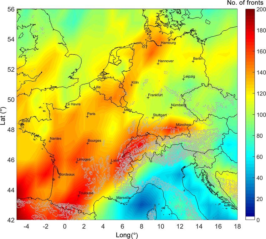
1872                                                                   M. Kunz et al.: Ambient conditions during hail events

Figure 1. Number of SCSs per year (center of each track) interpolated at 0.25◦ × 0.25◦ (color bar) and HSs (black dots) between 2005
and 2014 over the investigation area (France, Germany, Belgium, and Luxembourg).

2001; Kunz and Puskeiler, 2010; Piper et al., 2019), most of
these hotspots are located over and downstream of the moun-
tain ranges. Over France, SCS tracks are much more frequent
compared to Germany (Fig. 1). By contrast, HS tracks are far
more frequently detected over Germany due to more avail-
able reports. Nevertheless, Fig. 1 suggests a relationship be-
tween the two records: regions with an increased SCS fre-
quency also show an increased HS frequency and vice versa.

3.2    Daily and seasonal cycle

Both HS and SCS events (the latter not shown) feature pro-
nounced seasonal and diurnal cycles with a maximum in the
afternoon in the warmest months of July and August. While
the number of HSs is lowest in April and September and
dominated by smaller-sized hail, the months of May to July
are similar with the highest number of HS events of the di-
ameter class D ≥ 5 cm in June (Fig. 2a). A comparison of
the 3 summer months shows that events with large hail are
rarest in July. Reasons for this counterintuitive result might
be a decrease in frontal events, which have low hail sizes on
average (cf. Sect. 2.5.1), or reduced reporting in this month
due to summer vacations.                                            Figure 2. (a) Seasonal and (b) diurnal (local time; LT) cycle of HS
   The diurnal cycle is much more pronounced than the sea-          tracks (SHY of 2004–2014) depending on the hail size diameter
sonal cycle. The minimum number of HS events occurs in the          according to ESWD reports.
early morning hours between 03:00 and 09:00 LT, and the
maximum is in the afternoon between 15:00 and 18:00 LT
(Fig. 2b). The largest increase occurs between 12:00 and

Nat. Hazards Earth Syst. Sci., 20, 1867–1887, 2020                                  https://doi.org/10.5194/nhess-20-1867-2020
M. Kunz et al.: Ambient conditions during hail events 1873
15:00 LT, and the largest decrease is after 21:00 LT. A total During their propagation, cold fronts tend to weaken over
of 841 events, which correspond to 85.4 % of the HS sample, land mainly because of friction in the lowest layers and the
are registered in the period from 12:00 to 21:00 LT. horizontal mixing of air mass properties. Usually, they also
A separation of the diurnal cycle according to the hail di- dissolve when the air from the warm sector has entirely lifted
ameter shows that during the first half of the day (00:00– (occlusion). As the largest fraction of fronts affecting cen-
12:00 LT), most events are associated with hail smaller than tral Europe propagates in eastern to southeastern directions,
5 cm. Especially from 03:00 to 09:00 LT, hailstones are the their detectable density gradually decreases in the same di-
smallest of the entire day. This result, however, must be rection. In addition, an elevated front density can be found on
treated with care because of the low number of events in the western and northern side (upstream) of large mountains
that period (26 events) in combination with the potential un- such as the Pyrenees, Massif Central, and the Alps. These
derreporting by spotters in the night. During noon and after- large mountain ranges tend to slow down the propagation
noon, the proportion of hail with a diameter of at least 5 cm of fronts, leading to an elevated frequency upstream when
increases, and the highest probability of occurrence is be- counting the time steps where a front prevails (Schemm et al.,
tween 15:00 and 18:00 LT. In the evening and night (18:00– 2016). Thus, slowly propagating fronts may be repeatedly
00:00 LT), the relative proportion of large hail remains al- detected and counted during the time steps of ERA-Interim
most constant. (6 h). In contrast, fronts occur less frequently downstream of
The pronounced diurnal cycle of the HS probability larger mountains as well as at a greater distance to the sea,
(Fig. 2b) is closely linked to the warming of near-surface lay- where the increasing continentality acts to weaken or even
ers of air and the associated increase in lapse rate and CAPE dissolve the fronts.
together with a decrease in CIN (Markowski and Richardson,
2010). In addition, triggering mechanisms such as low-level 4.2 Occurrence of frontal SCS and HS tracks
flow convergence in the wake of thermally induced circula-
tion over complex terrain or inhomogeneities in land cover To assess the role of synoptic cold fronts in the probability
are also connected to the diurnal temperature cycle. Studies and properties of SCSs, we first discuss the spatial distribu-
using radar reflectivity or lightning detections found similar tion of the ratio of frontal SCSs relative to all SCS events.
diurnal cycles for most of the area except for the Mediter- This ratio is computed independently for each single grid
ranean (e.g., Wapler, 2013; Nisi et al., 2016; Piper and Kunz, point with a size of 0.5◦ × 0.5◦ . Averaged over the entire area
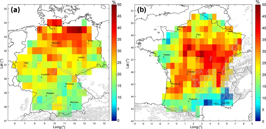
2017). of Germany and over the 10-year study period, 18.9 % of all
SCS tracks are related to a cold front; for France, the ratio
is slightly higher with 22.4 % (Fig. 4). The most conspicu-
4 SCSs associated with synoptic cold fronts ous feature in the spatial distribution of the frontal streaks
is the strong gradient in the south-to-north direction, particu-
Because of their relevance for SCS triggering, we investigate
larly over Germany. For example, while in the German north-
in the following the relation between synoptic cold fronts
east (Mecklenburg Lake Plateau) the share of frontal SCSs
with a significant length typically associated with extratrop-
reaches the highest value of 50 %, it decreases to less than
ical cyclones and SCS or HS events. Warm fronts are not
10 % in southern Germany over the Black Forest (southwest-
considered here because they are not important triggers for
ern Germany) and the region south of Nuremberg (southeast-
convection. This is mainly due to their reduced cross-frontal
ern Germany). Most striking in France is the extended max-
circulation and the resulting slow ascend, deduced through
imum of the frontal share of around 45 % northeast of the
the Sawyer–Eliassen equation (Emanuel, 1985), in combina-
domain’s center and several minima with only a few percent
tion with warm-air advection aloft, which has a stabilizing
near the coasts of both the North Atlantic and the Mediter-
effect. Because of their limitation to a specific territory, we
ranean.
also do not consider regional-scale land–sea contrasts, sea-
If we compare the proportion of frontal SCSs both with
breeze fronts, and thermal boundaries from Alpine pumping
the distribution of all SCS tracks (Fig. 1) and with the frontal
in the analysis.
density (Fig. 3), the opposite behavior is often observed. In
4.1 Cold-front climatology several regions with an increased number of fronts and/or
SCS events, the number of frontal SCSs is low and vice
The investigation area is frequently affected by synoptic- versa. This is especially true for Germany but also for parts
scale cold fronts. The number of fronts per grid point of the of France. Over complex terrain such as in southwestern Ger-
size 1◦ × 1◦ during the 10-year investigation period ranges many (Black Forest) or southern France (Massif Central),
between 85 in eastern Germany and 175 near the Pyrenees where frontal SCSs are comparatively rare, it can be assumed
(Fig. 3). Overall, front density in France is larger than in Ger- that orographically induced vertical lifting is often sufficient
many. to trigger convection so that a front is not necessary.
Considering HS instead of SCS events, we found that an
even higher number, namely 25 % of all HS tracks across the
https://doi.org/10.5194/nhess-20-1867-2020 Nat. Hazards Earth Syst. Sci., 20, 1867–1887, 2020
1874                                                                            M. Kunz et al.: Ambient conditions during hail events

Figure 3. Number of synoptic-scale fronts per 1◦ × 1◦ area between 2005 and 2014 (SHY) based on the ERA-Interim reanalysis according
to Schemm et al. (2015). Grey isolines represent the terrain (600, 1200, 1800, and 3600 m a.s.l.). Please note that the cities in this figure are
presented in their local names.

Figure 4. Share of frontal SCSs (relative to all SCSs; r ≤ 200 km) over (a) Germany and (b) France for 0.5◦ × 0.5◦ (SHY of 2005–2014).
Grid points containing less than 50 SCS tracks (see Fig. 1) were left white. Please note that the cities in this figure are presented in their local
names.

entire study domain, are connected to a synoptic cold front.                events are considered, the spatial distributions of frontal HS
Because of the small number of HS track detections, espe-                   and SCS tracks are quite similar.
cially in France (cf. Fig. 1), we do not show this relation here.             For the HS events, a relation is found between the length
Note, however, that if only areas with a sufficient number of               of the tracks as detected by the radar algorithm and the
                                                                            maximum observed hail diameter (Fig. 5a). While the mean

Nat. Hazards Earth Syst. Sci., 20, 1867–1887, 2020                                            https://doi.org/10.5194/nhess-20-1867-2020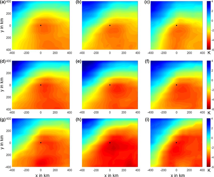
M. Kunz et al.: Ambient conditions during hail events                                                                                     1875

Figure 5. Boxplots showing (a) HS track lengths vs. maximum hail diameter according to ESWD reports and (b) maximum diameter (left)
and track length (right) for HS events with or without a synoptic-scale cold front. Indicated in the boxplots are the interquartile range (blue
box), median and mean values (red line and red x), and upper and lower 25 % percentile ± interquartile range × 1.5 (black lines); data points
outside of this range are marked as outliers (red crosses).

diameter for a length of L < 50 km is around 2 cm, it in-                 Table 1. Number of HS events in the respective classes of maximum
creases to around 3 cm for 50 ≥ L < 150 km and to 4 cm for                hail size diameter D and track length L.
L ≥ 150 km. Furthermore, the distributions of both quanti-
ties, maximum diameters and track lengths, differ between                                     L < 50 km     L = 50–100 km       L > 100 km
frontal and non-frontal streaks. Mean diameters are 3.3 cm                  D < 3 cm                 311                  98         64
in for frontal events and 2.73 cm for the others (Fig. 5b,                  D =3–4.5 cm              190                 102         72
left). For hail size diameter classes of < 2, 2–3.5, 4–5.5, and             D ≥ 5 cm                  63                  35         50
≥ 6 cm, the ratio between frontal and non-frontal events is
16.7 %, 23.1 %, 35.8 %, and 34.7 %, respectively (not shown;
note that the finer classes are used only in this example). This
means that the higher the probability of a nearby front is, the           > 100 km). When defining the threshold values, it was taken
larger the hailstone diameter is on average.                              into account that each class contains at least 50 events – ex-
   Differences between frontal and non-frontal HS events                  cept of the class L = 50–100 km and D ≥ 5 cm (Table 1). Us-
are also found for the length and mean propagation direc-                 ing other thresholds, for example, 150 km instead of 100 km
tion of the tracks. While frontal HS tracks have a mean                   as suggested by the diameter–length relation shown in the
length of 96.2 km (interquartile range of 40–125 km), non-                boxplot (Fig. 5), would result in sample sizes which were too
frontal tracks are almost half shorter with 56.8 km (25–                  small with less than 30 events. A further subdivision, for ex-
65 km; Fig. 5b, right part). Non-frontal HS events have a                 ample, according to the time of occurrence, was not carried
mean propagation angle of 215◦ (interquartile range 185–                  out. Although scientifically interesting, this would further re-
255◦ ), whereas those connected to a front propagate slightly             duce the sample sizes, particularly the most interesting high-
more to the east with a direction of 232◦ (interquartile range            intensity classes.
217–258◦ ; not shown). In that latter range of angles, also the
largest hailstones can be observed.                                       5.1   Mean composites of environmental conditions

                                                                          Averaged over all classes of HS events, SLI around the center
5   Environmental conditions of HS tracks                                 of the tracks has a mean value of −3.8 K (Fig. 6a), indicating
                                                                          a high potential for convective storms (e.g., Manzato, 2003;
Environmental conditions prevailing during HS events are in-              Kunz, 2007). SLI has its absolute minimum about 140 km
vestigated using SLI, DLS, and SRH from the ERA-Interim                   southeast of the events, but the difference to the center, on
reanalysis (see Sect. 2.2). The composites presented in the               average of 0.2 K, is almost negligible. Overall, a significant
following show the mean fields of the respective parameter                increase in convection-favoring conditions can be observed
around the center of the HS tracks (see Sect. 2.5.3). To ex-              from the northwest of the HS center to the southeast. While
amine environmental conditions depending on the intensity                 these conditions prevail over 400 km to the south and east of
of the HS events, we further divided the HS sample into nine              the center, the area to the north and west sees higher and
subsamples according to the observed hail diameter D (< 3,                positive values of SLI, thus stable conditions, at approxi-
3–4, and ≥ 5 cm) and track length L (< 50, 50–100, and                    mately 100–200 km distance already. The SLI field occurs

https://doi.org/10.5194/nhess-20-1867-2020                                        Nat. Hazards Earth Syst. Sci., 20, 1867–1887, 2020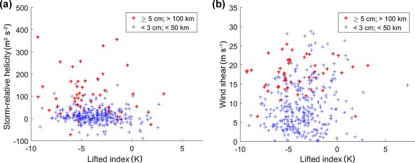
1876                                                                    M. Kunz et al.: Ambient conditions during hail events

rather smooth mainly because of the low resolution of ERA-           values of about 20 m s−1 and is thus in the range of the val-
Interim (cf. Sect. 5.3).                                             ues given in the literature (e.g., Weisman and Klemp, 1982;
   The vertical wind shear (DLS) has its maximum about               Thompson et al., 2007; Markowski and Richardson, 2010).
250 km to the west of the HS centers in an upstream direc-           The area of the highest DLS values is located several hun-
tion (Fig. 6b). This spatial difference is plausible because a       dred kilometers to the west of the HS events on average. For
trough frequently prevails to the west of the events. Since          large hail, the DLS maxima are even higher and further away
DLS is dominated by the wind speed aloft (500 hPa), a trough         from the HS events. These events are usually triggered by
with an associated jet manifests itself by a maximum in              upper-level troughs to the west, associated with higher wind
DLS. Considering the magnitude of DLS, it is found that              speed at mid-troposphere levels. One may argue that a rela-
the values are quite low with a mean of 12.5 m s−1 around            tionship between DLS and track length prevails per se, since
the HS events. Several authors have shown that organized             both are dominated by the wind speed aloft. Note, however,
convection capable of producing larger hail develops only in         that the separation of DLS applies not only to track length
sheared environments above around 10 m s−1 (e.g., Weisman            but also to storm duration (not shown here, but see Wandel,
and Klemp, 1982; Markowski and Richardson, 2010; Den-                2017).
nis and Kumjian, 2017). This is one of the reasons to further           In addition to DLS, SRH has been suggested by several
subdivide the whole sample as mentioned above and shown              authors (e.g., Thompson et al., 2007; Kunz et al., 2018) to
in the next paragraph.                                               be an important proxy not only for the prediction of tor-
                                                                     nadoes but also for large hail. In our composite analyses,
5.2    Environmental conditions depending on hail size               SRH (Fig. 9) shows even more pronounced differences be-
       and track length                                              tween the nine HS categories compared to DLS. Hail events
                                                                     with shorter tracks on average are in a range between 0 and
Separating the hail events according to their intensity allows       50 m2 s−2 . By contrast, longer tracks have much higher mean
for a detailed view of the prevailing environmental condi-           values between 84 and 116 m2 s−2 . According to the inves-
tions. The SLI composites show a slight decrease (higher in-         tigations of proximity soundings by Thompson et al. (2007),
stability) around the center of the HS events from small hail        such environments favor the development of weakly tornadic
with shorter tracks (SLI ≈ −3.7 K) to large hail with longer         and nontornadic supercells – provided that sufficient CAPE
tracks (SLI ≈ −4.5 K; Fig. 7). The strongest decrease in sta-        is present. In addition, there is also an increase in SRH from
bility occurs for increasing hail diameter, while the compos-        small to large hail, which is weaker compared to the trend in
ites are less sensitive to variations in track lengths. In all       the length classes. Interestingly, the highest SRH values oc-
cases, the lowest instability prevails to the southeast of the       cur directly at or near the location of the hail event and not
hail events as was already found for the mean composite              on the upstream side as was the case for DLS.
(cf. Fig. 6). Despite favorable environments for SCSs, which            To further investigate which of the dynamical parameters,
predominate all classes, the highest instability in the case of      SRH or DLS, best distinguishes the HS intensity, we con-
larger hail is an indicator of higher updraft speed within the       sider only the two categories that correspond to the highest
thunderstorm cloud, which is a prerequisite for the growth to        and lowest damage potentials: smaller hail with D < 3 cm
large hailstones.                                                    combined with short track length of L < 50 km and large
   The distance between the location of the events and the lo-       hail with D ≥ 5 cm combined with longer tracks of more
cation of the highest instability is greater for longer tracks       than 100 km (high-intensity events). Environmental param-
than for shorter ones but only in the case of small- to              eters are computed by the mean of the 3 × 3 ERA-Interim
medium-sized hail. At this point one may speculate that the          grid points centered around the HS locations.
reason for this shift might be related to the role of cold fronts,      Overall, the scatterplots presented in Fig. 10 show a much
considering that longer tracks and larger hailstones are more        clearer separation between the events when SRH is consid-
often connected to a cold front as discussed in the previous         ered (Fig. 10a) instead of DLS (Fig. 10b). About 50 % of
section (cf. Fig. 5). The role of cold fronts vs. environmental      the high-intensity events have values of 100 m2 s−2 or greater
conditions will be investigated in the next section.                 for SRH, while only 3 % of the low-intensity events display
   In contrast to the thermodynamical proxy SLI, the dynami-         these values. Furthermore, most of the latter events have val-
cal quantity DLS shows significantly pronounced differences          ues between −50 and 50 m2 s−2 . It can also be seen that SLI
between the nine HS categories (Fig. 8). Even though DLS             for all events in these two categories varies between 0 and
also distinguishes between the diameter classes, the largest         −10 K, with only a few exceptions having positive values.
differences are found for the three length classes. For exam-        Approximately 70 % of the high-intensity events have values
ple, DLS has a mean value of 17 m s−1 for long tracks in the         of −2.5 K or less. Unlike DLS (Fig. 10b), splitting the events
smallest diameter class (D < 3 cm), which is almost twice as         into two different categories is not possible. Even if most of
high compared to short tracks with the same diameter class           the high-intensity events form in an environment with DLS
(8.5 m s−1 ; Fig. 8, upper row). The same applies to the other       of at least 15 m s−1 (approx. 60 % of these events), there are
diameter classes. For long tracks with large hail, DLS reaches       still many low-intensity events for larger DLS values.

Nat. Hazards Earth Syst. Sci., 20, 1867–1887, 2020                                  https://doi.org/10.5194/nhess-20-1867-2020
M. Kunz et al.: Ambient conditions during hail events 1877
Figure 6. Composite analyses showing the average values of (a) SLI and (b) DLS from ERA-Interim in moving spatial windows centered at
the track location (center) for all 985 HS events between 2005 and 2014 (SHY; see Fig. 1).
Figure 7. Composite analyses of SLI related to maximum observed hail diameters of D < 3 cm (a–c), 3–4.5 cm (d–f), and ≥ 5 cm (g–i) and
for track lengths of L < 50 km (a, d, g), 50–100 km (b, e, h), and ≥ 100 km (c, f, i). The sizes of the subsamples are listed in Table 1.
5.3 Effects of model resolution on convective 2010), cannot be expected to be reproduced by the coarse
parameters ERA-Interim reanalysis. For this reason, we additionally
considered the high-resolution coastDat-3 reanalysis. Due to
the hourly resolved model fields, the maximum time differ-
Subgrid-scale spatial variations of the environmental condi- ence between the HS events and the environments is 30 min.
tions, for example, as a result of diabatic heating or temper- The purpose is not to reproduce the above analyses but to in-
ature and moisture advection (Markowski and Richardson,
https://doi.org/10.5194/nhess-20-1867-2020 Nat. Hazards Earth Syst. Sci., 20, 1867–1887, 20201878 M. Kunz et al.: Ambient conditions during hail events
Figure 8. Same as Fig. 7 but for 0–500 hPa DLS.
vestigate exemplarily the influence of the model resolution thermodynamic quantities such as the precipitable water (not
on the results. Since SLI and SRH are not available or quan- shown).
tifiable from coastDat-3, we used LR as a thermodynamical
proxy and DLS as a dynamical proxy (cf. Sect. 2.2). Because 5.4 Frontal vs. non-frontal HS tracks
the two proxies do not show significant differences between
the nine intensity categories (cf. Figs. 7 to 9), we discuss only As already discussed in Sect. 4.2, the characteristics of
the most severe HS category with L ≥ 100 km and D ≥ 5 cm. HS tracks having a front nearby substantially differ from
As shown in Fig. 11, the higher model resolution (right non-frontal events, especially with regard to the maximum
column) has little influence on the spatial distribution of the hail size and the track lengths (cf. Fig. 5). This suggests that
environmental parameters even though coastDat-3 compos- prevailing environmental conditions may likewise differ for
ites show a much larger spatial variability compared to ERA- the two kinds of events. Therefore, we further subdivided the
Interim. In the case of LR, the maximum is located to the HS sample into frontal and non-frontal types. To ensure that
southwest; in the case of DLS, it is located northeast of the enough events enter the subsamples, we made a further sep-
HS events as was already found in the above analyses. Also aration by considering only two length classes (L < 75 and
the distance between the maxima and the events remains al- ≥ 75 km) and two diameter classes (D < 3 and ≥ 3 cm; the
most the same. The coastDat-3 values around the maxima former not shown).
show a slight increase of approximately 10 % for both pa- Whereas the mean SLI composites are almost similar for
rameters. In the vicinity of the HS centers, the increase is frontal and non-frontal events (not shown), DLS shows sig-
only marginal but larger for LR compared to DLS. In partic- nificant differences between the four classes (Fig. 12). Over-
ular the LR increase is a consequence of the higher tempo- all, DLS reaches higher values with larger gradients for
ral resolution of coastDat-3 leading to an improved represen- frontal compared to non-frontal events (Fig. 12, panels a
tation of the diurnal temperature and moisture cycles. Note and c vs. b and d). However, when considering addition-
that this finding does not only apply to LR but also to other ally the track lengths, much larger differences in DLS can be
found, but only for non-frontal events (Fig. 12b and d). While
Nat. Hazards Earth Syst. Sci., 20, 1867–1887, 2020 https://doi.org/10.5194/nhess-20-1867-2020M. Kunz et al.: Ambient conditions during hail events 1879 Figure 9. Same as Fig. 7 but for 0–3 km SRH. Figure 10. Scatterplots between (a) SLI and SRH and (b) DLS for two different categories of track length and hail diameter. short non-frontal tracks form at a DLS value of 10.9 m s−1 on indication that frontal HS events preferably develop in pre- average, long tracks require medium-sheared environments, frontal environments (and not postfrontal). here with values of 15.9 m s−1 . A similar result is obtained for small hail sizes (D < 3 cm) with DLS even rising from 5.5 Differences in wind direction 9.0 to 16.7 m s−1 (not shown). Furthermore, while the DLS maximum for non-frontal events is located to the west of the It is well-known that supercells due to specific condi- center, it is more northwest for frontal events at a distance tions, such as a strong and spatially extended updraft, high of about 200 km. Since almost all synoptic fronts in Europe amounts of supercooled liquid water, or their longevity, propagate in a west–east direction, this location is a clear are capable to produce the largest hailstones (Foote, 1984; https://doi.org/10.5194/nhess-20-1867-2020 Nat. Hazards Earth Syst. Sci., 20, 1867–1887, 2020
1880                                                                     M. Kunz et al.: Ambient conditions during hail events

Figure 11. Composites of LR (a, b) and DLS (c, d) for hail diameters D ≥ 5 cm and track lengths L ≥ 100 km based on ERA-Interim (a, c)
and coastDat-3 (b, d) reanalyses.

Figure 12. Composites of DLS for maximum observed hail diameters D ≥ 3 cm and track lengths of L < 75 km (a, b) and L ≥ 75 km (c, d)
for frontal (a, c) and non-frontal (b, d) HS events.

Nat. Hazards Earth Syst. Sci., 20, 1867–1887, 2020                                   https://doi.org/10.5194/nhess-20-1867-2020
M. Kunz et al.: Ambient conditions during hail events 1881
Markowski and Richardson, 2010; Dennis and Kumjian, For example, as shown by Kunz and Puskeiler (2010), these
2017). The propagation of these highly organized convective hotspots are connected to flow convergence at lower lay-
systems can substantially deviate from the horizontal wind ers in the low-Froude-number regime, when the flow tends
at mid-tropospheric levels mainly because of the dynamics to go around rather than over the mountains. Overall, the
of the cold pools and induced vertical pressure deviations spatial distribution of SCS or HS events agrees with other
(Markowski and Richardson, 2010). studies on that topic considering different datasets such as
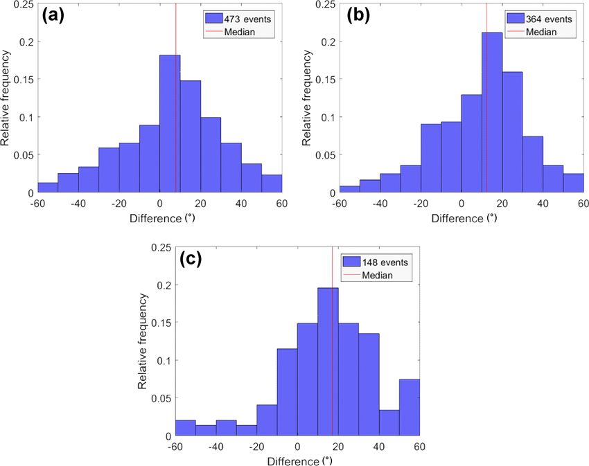
In the last step, therefore, we want to investigate whether 3D radar reflectivity (Kunz and Kugel, 2015; Puskeiler et al.,
our samples show a relation between the storm motion rela- 2016; Lukach et al., 2017), a combination of radar data with
tive to the mean wind and the hail size. The storm motion weather stations (Junghänel et al., 2016), or overshooting top
vector c follows from the radar tracking of the individual detections from satellites (Bedka, 2011; Punge et al., 2017).
HS events; the wind direction is estimated from the 500 hPa This applies also to the detected seasonal and diurnal cycles
mean wind from ERA-Interim (3 × 3 grid point around the (Nisi et al., 2016, 2018; Punge and Kunz, 2016). The good
HS centers). The cell-tracking algorithm (cf. Sect. 2.4) yields quantitative and qualitative agreement is a strong indication
very reliable shift vectors of individual hailstorms. The wind of the reliability of our methods and results.
field in 500 hPa, on the other hand, is mainly determined by All composites of environment parameters created for
the setting of the synoptic systems and only marginally af- radar-derived HS tracks show a similar spatial pattern:
fected by local-scale flow deviations. Positive differences in whereas the thermodynamic proxies such as SLI have their
the analyses indicate right-moving storms; negative values highest values at some 10 up to 100 km southeast of the cen-
indicate left-moving storms. ter of the HS events, the maxima of the dynamic proxies
Most of the events with smaller hail (D < 3 cm) propagate (DLS and SRH) are found to the northwest at a distance of
approximately parallel to the wind vectors in 500 hPa; the 100 to 200 km. This applies to all intensity classes and to all
mean difference between the tracks and the wind vectors is proxies originally considered in our study (also for the KO
only 8◦ (Fig. 13a). About 13 % of all HS events have a devi- index – Konvektiv-Index, convective index – and lapse rate
ation between 30 and 60◦ to the right, while only 6 % of the but not for precipitable water – PW, where the maximum is
events show deviations to the left for this interval (−30 to located north of the events).
−60◦ ). Hail events with maximum diameters between 3 and In total, 651 of the 985 HS events have a southwest-to-
4.5 cm show a deviation of the propagation direction prefer- northeast propagation direction, reflecting the mean flow di-
ably to the right of the wind vectors (Fig. 13b); 23 % of all rection at mid-troposphere levels. On average, HS events
HS events propagate with the wind in 500 hPa (decreasing by usually occur downstream of the eastern flank of a mid-
8 % compared to small hail), while 38 % of the tracks show troposphere trough, where southerly-to-southwesterly winds
a deviation between 10 and 30◦ . are frequently associated with the advection of unstable,
HS events of the largest hail class not only show an in- warm, and moist air masses from the Mediterranean (Graf
creased spread of the propagation deviation but also the en- et al., 2011; Wapler and James, 2015; Piper et al., 2019). This
tire histogram is shifted to more right-moving storms (me- constellation is often referred to as “Spanish plume” (Morris,
dian of 17◦ ; Fig. 13c). An angle difference between 10 and 1986). The trough, on the other hand, creates an environment
30◦ is observed for 35 % of all events. The largest difference with increased wind shear and large-scale lifting. The axis
to the other hail size classes is the comparatively high num- of the trough is usually located several hundred kilometers
ber of HS events between 30 and 60◦ (21 %). In contrast, upstream of the HS events, which explains why the highest
27 % of the events propagate with the wind in 500 hPa, and shear is found on the western flank at larger distances. Fur-
only 10 % have a negative deviation to the left of the wind in thermore, as convection initiation requires an additional lift-
500 hPa. In summary, the larger the hailstone diameters are, ing mechanism to overcome the convective inhibition in the
the stronger the deviation of the cell’s propagation direction planetary boundary layer, the area downstream of a trough
from the flow at 500 hPa is. is an ideal location for the development of (organized) con-
vection as shown, for example, by Wapler and James (2015),
Piper et al. (2019), or Mohr et al. (2020).
6 Discussion The separation of the environmental composites into dif-
ferent classes of hail diameter and track length yields sev-
Severe convective storms, chiefly hailstorms, are high- eral interesting results. Thermal instability, as expressed, for
frequent perils that, due to their local-scale nature, affect only example, by SLI, increases slightly (smaller values of SLI)
small areas (Changnon, 1977). Their reconstruction requires from small hail with shorter tracks to large hail with longer
high-resolution observational data such as radar reflectivity tracks, as might be expected. While the strongest decrease
used in our study. The results of the analyses show high spa- is found for increasing hail sizes, the composites are only
tial variability of both SCS and HS events, with a gradual marginally sensitive to variations in the track length. By con-
increase with growing distance from the ocean and several trast, the separation for DLS and SRH is much stronger, par-
hotspots, mainly over and downstream of mountain ranges. ticularly for the track lengths. This dependence of the track
https://doi.org/10.5194/nhess-20-1867-2020 Nat. Hazards Earth Syst. Sci., 20, 1867–1887, 2020You can also read