An empirical algorithm to map perennial firn aquifers and ice slabs within the Greenland Ice Sheet using satellite L-band microwave radiometry
←
→
Page content transcription
If your browser does not render page correctly, please read the page content below
The Cryosphere, 16, 103–125, 2022
https://doi.org/10.5194/tc-16-103-2022
© Author(s) 2022. This work is distributed under
the Creative Commons Attribution 4.0 License.

An empirical algorithm to map perennial firn aquifers and ice slabs
within the Greenland Ice Sheet using satellite L-band microwave
radiometry
Julie Z. Miller1,2 , Riley Culberg3 , David G. Long4 , Christopher A. Shuman5 , Dustin M. Schroeder3,6 , and
Mary J. Brodzik1,7
1 Cooperative  Institute for Research in Environmental Sciences, University of Colorado Boulder, Boulder, Colorado, USA
2 Earth Science and Observation Center, University of Colorado Boulder, Boulder, Colorado, USA
3 Department of Electrical Engineering, Stanford University, Stanford, California, USA
4 Department of Electrical and Computer Engineering, Brigham Young University, Provo, Utah, USA
5 Joint Center for Earth Systems Technology at Code 615, Cryospheric Sciences Laboratory, NASA Goddard Space Flight

Center, University of Maryland, Baltimore County, Greenbelt, Maryland, USA
6 Department of Geophysics, Stanford University, Stanford, CA, USA
7 National Snow and Ice Data Center, University of Colorado Boulder, Boulder, Colorado, USA

Correspondence: Julie Z. Miller (jzmiller.research@gmail.com)

Received: 21 April 2021 – Discussion started: 30 April 2021
Revised: 1 December 2021 – Accepted: 1 December 2021 – Published: 13 January 2022

Abstract. Perennial firn aquifers are subsurface meltwater         percolation facies of the GrIS that can be defined primarily
reservoirs consisting of a meters-thick water-saturated firn       by differences in snow accumulation, which influences the
layer that can form on spatial scales as large as tens of          englacial hydrology and thermal characteristics of firn layers
kilometers. They have been observed within the percola-            at depth.
tion facies of glaciated regions experiencing intense seasonal        Here, for the first time, we use enhanced-resolution ver-
surface melting and high snow accumulation. Widespread             tically polarized L-band brightness temperature (TVB ) im-
perennial firn aquifers have been identified within the Green-     agery (2015–2019) generated using observations collected
land Ice Sheet (GrIS) via field expeditions, airborne ice-         over the GrIS by NASA’s Soil Moisture Active Passive
penetrating radar surveys, and satellite microwave sensors.        (SMAP) satellite to map perennial firn aquifer and ice slab
In contrast, ice slabs are nearly continuous ice layers that can   areas together as a continuous englacial hydrological sys-
also form on spatial scales as large as tens of kilometers as      tem. We use an empirical algorithm previously developed
a result of surface and subsurface water-saturated snow and        to map the extent of Greenland’s perennial firn aquifers
firn layers sequentially refreezing following multiple melt-       via fitting exponentially decreasing temporal L-band signa-
ing seasons. They have been observed within the percola-           tures to a set of sigmoidal curves. This algorithm is recali-
tion facies of glaciated regions experiencing intense seasonal     brated to also map the extent of ice slab areas using airborne
surface melting but in areas where snow accumulation is at         ice-penetrating radar surveys collected by NASA’s Opera-
least 25 % lower as compared to perennial firn aquifer areas.      tion IceBridge (OIB) campaigns (2010–2017). Our SMAP-
Widespread ice slabs have recently been identified within the      derived maps show that between 2015 and 2019, perennial
GrIS via field expeditions and airborne ice-penetrating radar      firn aquifer areas extended over 64 000 km2 , and ice slab
surveys, specifically in areas where perennial firn aquifers       areas extended over 76 000 km2 . Combined together, these
typically do not form. However, ice slabs have yet to be           sub-facies are the equivalent of 24 % of the percolation fa-
identified from space. Together, these two ice sheet features      cies of the GrIS. As Greenland’s climate continues to warm,
represent distinct, but related, sub-facies within the broader     seasonal surface melting will increase in extent, intensity,

Published by Copernicus Publications on behalf of the European Geosciences Union.
104                                                          J. Z. Miller et al.: Mapping perennial firn aquifers and ice slabs

and duration. Quantifying the possible rapid expansion of           aquifers just prior to melt onset ranges from between 10 %
these sub-facies using satellite L-band microwave radiometry        and 25 %, which limits the upward propagation of electro-
has significant implications for understanding ice-sheet-wide       magnetic energy from greater depths within the ice sheet.
variability in englacial hydrology that may drive meltwater-        Large volumetric fractions of meltwater within the firn pore
induced hydrofracturing and accelerated ice flow as well as         space result in high reflectivity and attenuation at the inter-
high-elevation meltwater runoff that can impact the mass bal-       face between water-saturated firn layers and the overlying re-
ance and stability of the GrIS.                                     frozen firn layers as well as between glacial ice or an imper-
                                                                    meable layer and the overlying water-saturated firn layers.
                                                                    Upwelling L-band emission from deeper glacial ice and the
                                                                    underlying bedrock is effectively blocked.
1   Introduction                                                       While perennial firn aquifers are radiometrically cold, the
                                                                    slow refreezing of deeper firn layers saturated with large vol-
The recent launches of several satellite L-band microwave           umetric fractions of meltwater represents a significant source
radiometry missions by NASA (Aquarius mission, Le Vine              of latent heat that is continuously released throughout the
et al., 2007; Soil Moisture Active Passive (SMAP) mission,          freezing season. Refreezing of seasonal meltwater by the
Entekhabi et al., 2010) and ESA (Soil Moisture and Ocean            descending winter cold wave (Pfeffer et al., 1991), and the
Salinity (SMOS), Kerr et al., 2001) have provided a new             subsequent formation of embedded ice structures (i.e., hor-
Earth-observation tool capable of detecting meltwater stored        izontally oriented ice layers and ice lenses as well as verti-
tens of meters to kilometers beneath the ice sheet surface.         cally oriented ice pipes; Benson et al., 1960; Humphrey et
Jezek et al. (2015) recently demonstrated that in the high-         al., 2012; Harper et al., 2012) within the upper snow and firn
elevation (3500 m a.s.l.) dry snow facies of the Antarctic Ice      layers, represents a secondary source of latent heat. These
Sheet, meltwater stored in subglacial Lake Vostok can be de-        heat sources help maintain meltwater at depth. Perennial firn
tected as deep as 4 km beneath the ice sheet surface. Sub-          aquifer areas are radiometrically warmer than other percola-
glacial lakes represent radiometrically cold subsurface melt-       tion facies areas where the single source of latent heat is via
water reservoirs. Upwelling L-band emission from the radio-         refreezing of seasonal meltwater. This results in a higher ob-
metrically warm bedrock underlying the subglacial lakes is          served T B at the ice sheet surface during the freezing season
effectively blocked by high reflectivity and attenuation at the     as compared to other percolation facies areas where seasonal
interface between the bedrock and the overlying lake bottom.        meltwater is fully refrozen and stored exclusively as embed-
This results in a lower observed microwave brightness tem-          ded ice.
perature (T B ) at the ice sheet surface as compared to other          Recently, mapping the extent of Greenland’s perennial
dry snow facies areas where bedrock contributes to L-band           firn aquifers from space was demonstrated using satellite
emission depth-integrated over the entire ice sheet thickness.      L-band microwave radiometry (Miller et al., 2020). Expo-
   Similar to subglacial lakes, perennial firn aquifers also        nentially decreasing temporal L-band signatures observed
represent radiometrically cold subsurface meltwater reser-          in enhanced-resolution vertically polarized L-band bright-
voirs (Miller et al., 2020) consisting of a 4–25 m thick water-     ness temperature (TVB ) imagery (2015–2016) generated using
saturated firn layer (Koenig et al., 2014; Montgomery et al.,       observations collected over the GrIS by the microwave ra-
2017; Chu et al., 2018) that can form on spatial scales as large    diometer on NASA’s SMAP satellite (Long et al., 2019) were
as tens of kilometers (Forster et al., 2014). Perennial firn        correlated with a single year of perennial firn aquifer detec-
aquifers have been identified via field expeditions (Forster        tions (Miège et al., 2016). These detections were identified
et al., 2014), airborne ice-penetrating radar surveys (Miège        via the Center for Remote Sensing of Ice Sheets (CReSIS)
et al., 2016), and satellite microwave sensors (Brangers et         Multi-Channel Coherent Radar Depth Sounder (MCoRDS)
al., 2020; Miller et al., 2020) in the lower-elevation (<           flown by NASA’s Operation IceBridge (OIB) campaigns
2000 m a.s.l.) percolation facies of the Greenland Ice Sheet        (Rodriguez-Morales et al., 2014). An empirical algorithm to
(GrIS) at depths from between 1 and 40 m beneath the ice            map extent was developed by fitting temporal L-band signa-
sheet surface. They exist in areas that experience intense          tures to a set of sigmoidal curves derived from the continuous
seasonal surface melting and rain (> 650 mm w.e. yr−1 ) dur-        logistic model.
ing the melting season and high snow accumulation (>                   The relationship between the radiometric, and thus the
800 mm w.e. yr−1 ) during the freezing season (Forster et al.,      physical, temperature of perennial firn aquifer areas, as com-
2014). High snow accumulation in perennial firn aquifer ar-         pared to other percolation facies areas, forms the basis of the
eas thermally insulates water-saturated firn layers from the        empirical algorithm. Miller et al. (2020) hypothesized that
cold atmosphere, allowing seasonal meltwater to be stored in        the dominant control on the relatively slow exponential rate
liquid form year-round if the overlying seasonal snow layer is      of T B decrease over perennial firn aquifer areas is physical
sufficiently thick (Kuipers Munneke et al., 2014). Koenig et        temperature versus depth. L-band emission from the radio-
al. (2014) estimated that the volumetric fraction of meltwa-        metrically warm upper snow and firn layers decreases dur-
ter stored within the pore space of Greenland’s perennial firn      ing the freezing season as embedded ice structures slowly re-

The Cryosphere, 16, 103–125, 2022                                                       https://doi.org/10.5194/tc-16-103-2022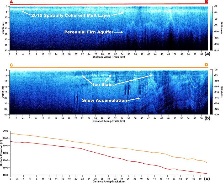
J. Z. Miller et al.: Mapping perennial firn aquifers and ice slabs                                                              105

freeze at increased depths below the ice sheet surface. In the      2     Methods
percolation facies, refreezing of seasonal meltwater results in
the formation of an intricate network of embedded ice struc-        We adapt our previously developed empirical algorithm to
tures that are large (10–100 cm long, 10–20 cm wide; Jezek          map the extent of Greenland’s perennial firn aquifers (Miller
et al., 1994) relative to the L-band wavelength (21 cm). Em-        et al., 2020) using a multi-year calibration technique. We
bedded ice structures induce strong volume scattering (Rig-         use enhanced-resolution L-band TVB imagery (2015–2019)
not et al., 1993; Rignot, 1995) that decreases T B (Zwally,         generated using observations collected over the GrIS by the
1977; Swift et al., 1985; Jezek et al., 2018).                      microwave radiometer on NASA’s SMAP satellite (Long et
   Ice slabs are 1–16 m thick nearly continuous ice layers that     al., 2019) and airborne ice-penetrating radar surveys col-
can form on spatial scales as large as tens of kilometers as        lected by NASA’s OIB campaigns (Rodriguez-Morales et al.,
a result of surface and subsurface water-saturated snow and         2014). First, we correlate (1) a “firn saturation” parameter de-
firn layers sequentially refreezing following multiple melting      rived from a simple two-layer L-band brightness temperature
seasons (Machguth et al., 2016; MacFerrin et al., 2019). Over       model; (2) maximum and (3) minimum TVB values; and (4)
time, they become dense low-permeability solid-ice layers           exponentially decreasing temporal L-band signatures, with
overlying deeper permeable firn layers. Ice slabs have been         5 years of perennial firn aquifer detections (2010–2014) iden-
identified via field expeditions and airborne ice-penetrating       tified via the CReSIS Accumulation Radar (AR) (Miège et
radar surveys in the lower-elevation (< 2000 m a.s.l.) perco-       al., 2016) and 3 years of additional detections (2015–2017)
lation facies of the GrIS at depths from between 1 and 20 m         more recently identified via MCoRDS (Miller et al., 2020).
beneath the ice sheet surface (MacFerrin et al., 2019). They        Next, we extend our empirical algorithm to map the extent
exist in areas that experience intense seasonal surface melt-       of ice slab areas. We correlate the SMAP-derived parame-
ing and rain (excess melt of 266–573 mm w.e. yr−1 ; see Mac-        ters with 5 years of ice slab detections (2010–2014) recently
Ferrin et al., 2019, for a description) during the melting sea-     identified via AR (MacFerrin et al., 2019). Finally, we re-
son and lower snow accumulation (< 572±32 mm w.e. yr−1 )            calibrate our empirical model to map the extent of perennial
during the freezing season as compared to perennial firn            firn aquifer and ice slab areas over the percolation facies. In-
aquifer areas (MacFerrin et al., 2019). Lower snow accumu-          terannual variability in extent is not resolved in this study;
lation in ice slab areas results in a seasonal snow layer that is   however, it will be explored further in future work.
insufficiently thick to thermally insulate water-saturated firn
layers and seasonal meltwater is instead stored as embedded         2.1    SMAP enhanced-resolution L-band T B imagery
ice.
   Refreezing of seasonal meltwater by the descending win-          The key science objectives of NASA’s SMAP mission (https:
ter cold wave, and the subsequent formation of ice slabs as         //smap.jpl.nasa.gov/, last access: 4 January 2022) are to map
well as other embedded ice structures within the upper snow         terrestrial soil moisture and freeze/thaw state over Earth’s
and firn layers, is the single source of latent heat. While ice     land surfaces from space. However, the global L-band T B
slab areas are radiometrically warmer than other percolation        observations collected by the SMAP satellite also have
facies areas with a lower volumetric fraction of embedded           cryospheric applications. Mapping perennial firn aquifer and
ice, they are radiometrically colder than perennial firn aquifer    ice slab areas over Earth’s polar ice sheets represents an inter-
areas. This results in typically higher observed T B at the ice     esting analog and an innovative extension of the SMAP mis-
sheet surface during the freezing season in ice slab areas,         sion’s science objectives. The SMAP satellite was launched
as compared to other percolation facies areas, but typically        on 31 January 2015 and carries a microwave radiometer that
lower observed T B as compared to perennial firn aquifer ar-        operates at an L-band frequency of 1.41 GHz (Enkentabi et
eas. Similar to temporal L-band signatures over perennial firn      al., 2010). It is currently collecting observations of vertically
aquifer areas, temporal L-band signatures over ice slab ar-         and horizontally polarized T B over Greenland. The surface
eas are exponentially decreasing during the freezing season;        incidence angle is 40◦ , and the radiometric accuracy is ap-
however, the rate of T B decrease is slightly more rapid.           proximately 1.3 K (Piepmeier et al., 2017).
   In this study, we exploit the observed sensitivity of L-band        The Scatterometer Image Reconstruction (SIR) algorithm
emission to variability in the depth- and time-integrated di-       was originally developed to reconstruct coarse-resolution
electric and geophysical properties of the percolation facies       satellite radar scatterometry imagery on a higher-spatial-
of the GrIS to map perennial firn aquifer and ice slab areas        resolution grid (Long et al., 1993; Early and Long, 2001).
together as a continuous englacial hydrological system using        The SIR algorithm has been adapted for coarse-resolution
satellite L-band microwave radiometry.                              satellite microwave radiometry imagery (Long and Daum,
                                                                    1998; Long and Brodzik, 2016; Long et al., 2019). The mi-
                                                                    crowave radiometer form of the SIR algorithm (rSIR) uses
                                                                    the measurement response function (MRF) for each observa-
                                                                    tion, which is a smeared version of the antenna pattern. Us-
                                                                    ing the overlapping MRFs, the rSIR algorithm reconstructs

https://doi.org/10.5194/tc-16-103-2022                                                       The Cryosphere, 16, 103–125, 2022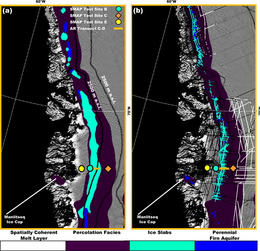
106                                                           J. Z. Miller et al.: Mapping perennial firn aquifers and ice slabs

T B from the spatially filtered low-resolution sampling pro-         face with no appreciable layover. The MCoRDS instrument
vided by the observations. In effect, it generates an MRF-           operated at three different frequency configurations: (1) a
deconvolved T B image. Combining multiple orbital passes             center frequency of 195 MHz with a bandwidth of 30 MHz
increases the sampling density, which improves both the ac-          (2010–2014, 2017), (2) a center frequency of 315 MHz with
curacy and resolution of the SMAP enhanced-resolution T B            a bandwidth of 270 MHz (2015), and (3) a center frequency
imagery (Long et al., 2019).                                         of 300 MHz with a bandwidth of 300 MHz (2016). The ver-
   Over Greenland, the rSIR algorithm combines satellite or-         tical range resolution in firn for each of these frequency con-
bital passes that occur between 08:00 and 16:00 local time           figurations is 5.3, 0.59, and 0.53 m, respectively (CReSIS,
of day to reconstruct SMAP enhanced-resolution T B im-               2016). The collected data have an along-track resolution of
agery twice-daily (i.e., morning and evening orbital pass in-        approximately 25 m with 14 m spacing between traces in the
terval, respectively). T B imagery is projected on a Northern        final processed radargrams. At the same nominal flight alti-
Hemisphere (NH) Equal-Area Scalable Earth Grid (EASE-                tude of 500 m, the cross-track resolution varies between 40 m
Grid 2.0; Brodzik et al., 2012) at a 3.125 km rSIR grid cell         for a smooth surface in the highest bandwidth configuration
spacing (e.g., Fig. 1). The effective resolution for each grid       and 175 m for a rough surface with no appreciable layover in
cell is dependent on the number of observations used in              the lowest bandwidth configuration.
the rSIR reconstruction and is coarser than the rSIR grid               The multi-year calibration technique uses perennial firn
cell spacing. While the effective resolution of convention-          aquifer detections previously identified along OIB flight
ally processed SMAP T B imagery posted on a 25 km grid               lines via AR (2010–2014) and MCoRDS (2015–2017) radar-
is approximately 30 km (e.g., Fig. 1a), the effective resolu-        gram profiles and the methodology described in Miège et
tion of SMAP enhanced-resolution T B imagery posted on a             al. (2016). Bright lower reflectors that undulate with the lo-
3.125 km grid is approximately 18 km (e.g., Fig. 1b), an im-         cal topographic gradient underneath which reflectors are ab-
provement of 60 % (Long et al., 2019).                               sent in the percolation facies are interpreted as the upper sur-
   As previously noted, for our analysis of the percolation          face of meltwater stored within perennial firn aquifers (e.g.,
facies we use SMAP enhanced-resolution TVB imagery over              Fig. 3a). The large dielectric contrast between refrozen and
the GrIS. Compared to the horizontally polarized channel,            water-saturated firn layers results in high reflectivity at the
the vertically polarized channel exhibits decreased sensitiv-        interface. However, the presence of meltwater increases at-
ity to variability in the volumetric fraction of meltwater,          tenuation, limiting the downward propagation of electromag-
which is attributed to reflection coefficient differences be-        netic energy through the water-saturated firn layer. The to-
tween channels (Miller et al., 2020). Using the vertically po-       tal number of AR derived perennial firn aquifer detections is
larized channel also results in a reduced chi-squared error          325 000, corresponding to a total extent of 98 km2 . The anal-
statistic when fitting TVB time series to the sigmoid function       ysis assumes a smooth surface, which is typical of much of
(Sect. 2.3.4). We construct TVB imagery that alternates morn-        the percolation facies, and a grid cell size of 15 m×20 m. The
ing and evening orbital pass observations annually, begin-           total number of MCoRDS-derived perennial firn aquifer de-
ning and ending just prior to melt onset. The Greenland Ice          tections is 142 000, corresponding to a total extent of 80 km2 .
Mapping Project (GIMP) Land Ice and Ocean Classification             This analysis also assumes a smooth surface and a grid cell
Mask and Digital Elevation Model (Howat et al., 2014) are            size of 14 m × 40 m. The combined total number of grid
projected on the NH EASE-Grid 2.0 at a 3.125 km rSIR grid            cells (467 000) and total extent (178 km2 ) is significantly
cell spacing. The derived ice mask includes the Greenland            larger than the total number of MCoRDS-derived grid cells
Ice Sheet and the peripheral ice caps, including Maniitsoq           (78 000) and total extent (44 km2 ) calculated for 2016 (Miller
and Flade Isblink. TVB imagery between 1 April 2015 and 31           et al., 2020). Perennial firn aquifer detections are mapped in
March 2019 is ice-masked, and an elevation for each rSIR             northwestern, southern, and south and central eastern Green-
grid cell is calculated.                                             land as well as the Maniitsoq and Flade Isblink ice caps
                                                                     (Figs. 1c and 2a).
2.2   Airborne ice-penetrating radar surveys                            We project AR- and MCoRDS-derived perennial firn
                                                                     aquifer detections on the NH EASE-Grid 2.0 at an rSIR grid
AR and MCoRDS (Rodriguez-Morales et al., 2014) were                  cell spacing of 3.125 km. Each rSIR grid cell has an extent of
flown over the GrIS on a P-3 aircraft in April and May be-           approximately 10 km2 . The total number of rSIR grid cells
tween 2010 and 2017. The AR instrument operates at a center          with at least one perennial firn aquifer detection is 800, cor-
frequency of 750 MHz with a bandwidth of 300 MHz, result-            responding to a total extent of 8000 km2 . However, given
ing in a range resolution in firn of 0.53 m (Lewis et al., 2015).    the limited AR and MCoRDS grid cell coverage, less than
The collected data have an along-track resolution of approx-         1 % of the rSIR grid cell extent has airborne ice-penetrating
imately 30 m with 15 m spacing between traces in the final           radar survey coverage. As compared to the total number of
processed radargrams. At a nominal flight altitude of 500 m          MCoRDS-derived perennial firn aquifer detections (780) cal-
above the ice sheet surface, the cross-track resolution varies       culated for 2016 (Miller et al., 2020), the total number of
between 20 m for a smooth surface and 54 m for a rough sur-          rSIR grid cells with at least one detection is only increased

The Cryosphere, 16, 103–125, 2022                                                         https://doi.org/10.5194/tc-16-103-2022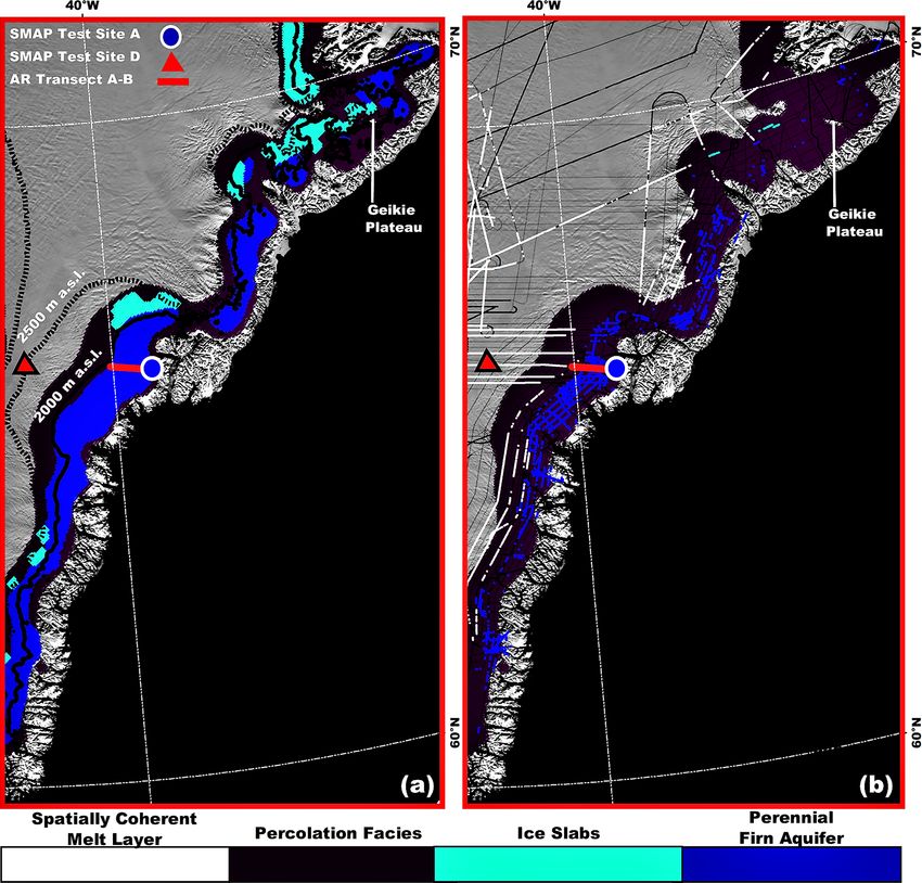
J. Z. Miller et al.: Mapping perennial firn aquifers and ice slabs 107
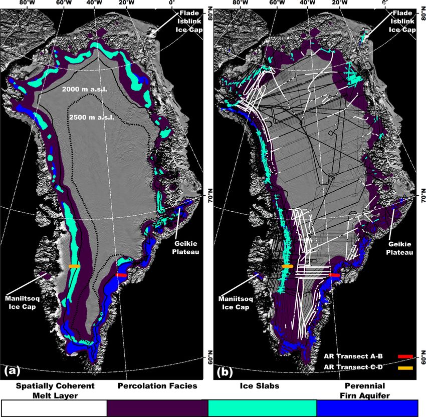
Figure 1. (a) Gridded (25 km gridding, 30 km effective resolution) and (b) enhanced-resolution (3.125 km gridding, 18 km effective resolu-
tion) L-band TVB imagery generated using observations collected on 15 April 2016 by the microwave radiometer on the SMAP satellite during
the evening orbital pass interval over Greenland (Long et al., 2019) overlaid with the 2000 m a.s.l. contour (black line) and the 2500 m a.s.l.
contour (dotted black line; Howat et al., 2014), the ice sheet extent (purple line; Howat et al., 2014), and the coastline (black peripheral line;
Wessel and Smith, 1996). (c) SMAP enhanced-resolution L-band TVB imagery overlaid with AR- and MCoRDS-derived 2010–2017 perennial
firn aquifer (blue shading; Miège et al., 2016), 2010–2014 ice slab (cyan shading; MacFerrin et al., 2019), and 2012 spatially coherent melt
layer (white shading; Culberg et al., 2021) detections along OIB flight lines (black interior lines); zoom areas over southeastern Greenland
(red box; Fig. 2a) and southwestern Greenland (orange box; Fig. 2b); and AR radargram transect A-B (red line; Fig. 3a) and C-D (orange
line; Fig. 3b).
by 20 for the multi-year calibration technique, corresponding We project the AR-derived ice slab detections on the NH
to an increased total extent of 200 km2 . EASE-Grid 2.0 at an rSIR grid cell spacing of 3.125 km. The
We also use ice slab detections previously identified along total number of rSIR grid cells with at least one ice slab de-
OIB flight lines via AR (2010–2014) radargram profiles and tection is 2000, corresponding to a total extent of 20 000 km2 .
the methodology described in MacFerrin et al. (2019) in the However, less than 2 % of the rSIR grid cell extent has air-
multi-year calibration technique. Thick dark surface-parallel borne ice-penetrating radar survey coverage.
regions of low reflectivity in the percolation facies are inter- An advantage of the multi-year calibration technique as
preted as ice slabs (e.g., Fig. 3b). The large dielectric contrast compared to the single-coincident year calibration technique
between ice slabs and the overlying and underlying snow (Miller et al., 2020) is that it increases the number of rSIR
and firn layers results in high reflectivity at the interfaces. grid cells that can be assessed. It also provides repeat tar-
However, electromagnetic energy is not scattered or absorbed gets that can account for variability in the depth- and time-
within the homogeneous ice slab; it instead propagates down- integrated dielectric and geophysical properties that influ-
ward through the layer and into the deeper firn layers. The to- ence the radiometric temperature in stable perennial firn
tal number of AR-derived ice slab detections is 505 000, cor- aquifer and ice slab areas. Uncertainty is introduced by
responding to a total extent of 283 km2 . Ice slab detections correlating the SMAP-derived parameters with AR- and
are mapped in western, central and northeastern, and north- MCoRDS-derived detections that are not coincident in time.
ern Greenland as well as the Flade Isblink Ice Cap (Figs. 1c The multi-year calibration technique assumes the extent of
and 2b). each area remains stable, which is not necessarily the case
as climate extremes (Cullather et al., 2020) can influence
https://doi.org/10.5194/tc-16-103-2022 The Cryosphere, 16, 103–125, 2022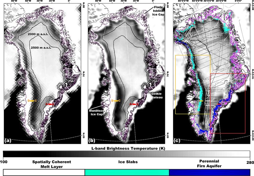
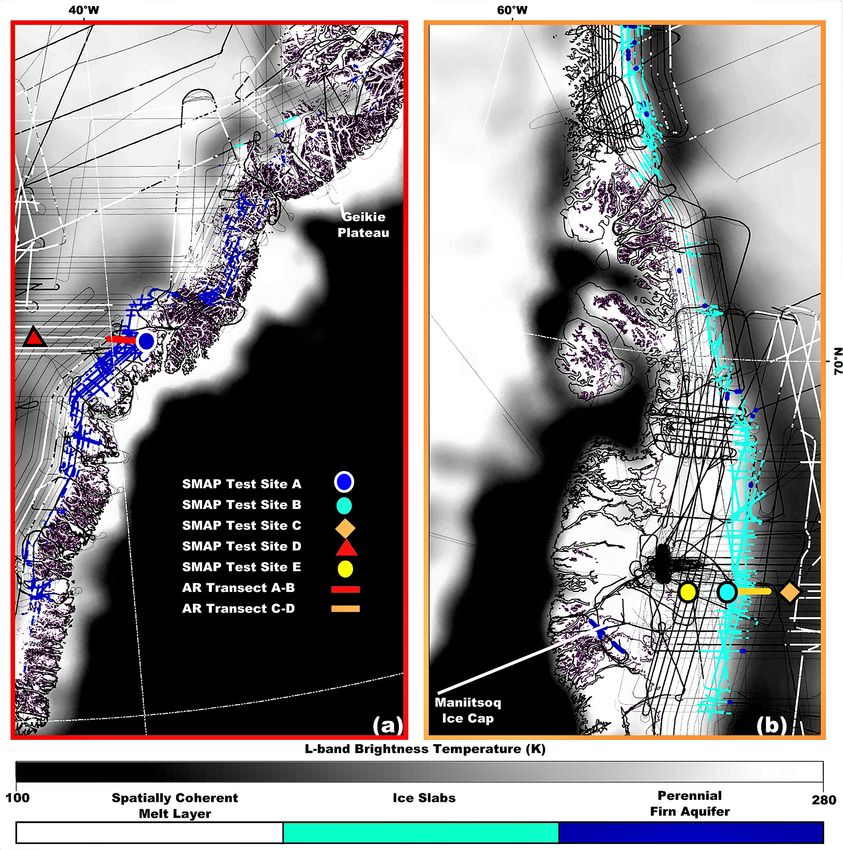
108                                                              J. Z. Miller et al.: Mapping perennial firn aquifers and ice slabs

Figure 2. Enhanced-resolution (3.125 km gridding, 30 km effective resolution) L-band TVB imagery generated using observations collected
on 15 April 2016 by the microwave radiometer on the SMAP satellite during the evening orbital pass interval over (a) southeastern Greenland
(red box; Fig. 1c) and (b) southwestern Greenland (orange box; Fig. 1c,) (Long et al., 2019) overlaid with the ice sheet extent (purple line;
Howat et al., 2014); the coastline (black peripheral line; Wessel and Smith, 1996); the AR- and MCoRDS-derived 2010–2017 perennial firn
aquifer (blue shading; Miège et al., 2016), 2010–2014 ice slab (cyan shading; MacFerrin et al., 2019), and 2012 spatially coherent melt layer
(white shading; Culberg et al., 2021) detections along OIB flight lines (black interior lines); AR radargram transect A-B (red line; Fig. 3a)
and C-D (orange line; Fig. 3b); and SMAP Test Site A (blue circle; Fig. 4a), B (cyan circle; Fig. 4b), C (orange diamond; Fig. 4c), D (red
triangle; Fig. 4d), and E (yellow circle; Fig. 4e).

each of these sub-facies. The assumption of stability neglects           formation of each of these sub-facies, with continued pres-
boundary transitions in the extent of perennial firn aquifer ar-         ence dependent on seasonal surface melting and snow accu-
eas associated with refreezing of shallow water-saturated firn           mulation in subsequent years.
layers, englacial drainage of meltwater into crevasses at the               Annual perennial firn aquifer and ice slab detections that
periphery (Poinar et al., 2017, 2019), and transient upslope             may introduce significant uncertainty into the multi-year cal-
expansion (Montgomery et al., 2017). Once formed, ice slabs              ibration technique include those following the 2010 melting
are essentially permanent features within the upper snow and             season, which was exceptionally long (Tedesco et al., 2011);
firn layers of the percolation facies until they are compressed          the anomalous 2012 melting season, during which seasonal
into glacial ice. However, they may transition into superim-             surface melting extended across 99 % of the GrIS (Nghiem
posed ice at the lower boundary of ice slab areas or rapidly             et al., 2012); and the 2015 melting season, which was espe-
expand upslope, particularly following extreme melting sea-              cially intense in western and northern Greenland (Tedesco
sons (MacFerrin et al., 2019). Thus, we simply consider our              et al., 2016). Following these extreme melting seasons, sig-
mapped extent a high-probability area for the preferential               nificant changes in the dielectric and geophysical properties

The Cryosphere, 16, 103–125, 2022                                                              https://doi.org/10.5194/tc-16-103-2022
J. Z. Miller et al.: Mapping perennial firn aquifers and ice slabs                                                                              109

Figure 3. AR radargram transect (a) A-B (red line; Fig. 2a) collected on 22 April 2017 and (b) C-D (orange line; Fig. 2b) collected on 5 May
2017 (Rodriguez-Morales et al., 2014). (c) AR radargram transect A-B (red line) and C-D (orange line) elevation profiles. The exceptionally
bright upper surface-parallel reflector in panel (a) is a spatially coherent melt layer. The bright lower reflector in panel (a) is the upper surface
of meltwater stored within a perennial firn aquifer. The thick dark surface-parallel regions of low reflectivity in panel (b) are ice slabs. The
alternating sequences of bright and dark surface-parallel reflectors in panel (b) are seasonal snow accumulation layers.

likely occurred across large portions of the GrIS, includ-                   sparsely connected via vertically oriented ice pipes (Culberg
ing perennial firn aquifer recharging resulting in increases                 et al., 2021). Spatially coherent melt layers are relatively thin
in meltwater volume and decreases in the depth to the upper                  (0.2 cm–2 m) and can rapidly form across the high-elevation
surface of stored meltwater. The upper snow and firn layers                  (up to 3200 m a.s.l.) dry snow facies at depths of less than
of the dry snow facies and percolation facies were also sat-                 1 m beneath the ice sheet surface following a single extreme
urated with relatively large volumetric fractions of meltwa-                 melting season. They can further merge together into thicker
ter as compared to the negligible-to-limited volumetric frac-                solid-ice layers following multiple extreme melting seasons.
tions of meltwater that percolates during more typical sea-                  Spatially coherent melt layers are exceptionally bright in AR
sonal surface melting over the GrIS.                                         radargrams (e.g., Fig. 3a). The large dielectric contrast be-
   Seasonal meltwater was refrozen into spatially coherent                   tween the spatially coherent melt layer and the overlying,
melt layers following the 2010 and 2012 melting seasons                      underlying, and interior snow and firn layers results in high
(Culberg et al., 2021) as well as more recently following the                reflectivity at the interfaces. However, electromagnetic en-
2015 and 2018 melting seasons identified as part of the tem-                 ergy still propagates downward through the high-reflectivity
poral L-band signature analysis in this study (Sect. 2.3.1).                 layer into the deeper firn layers. Culberg et al. (2021) recently
As compared to ice slabs, which are dense low-permeability                   demonstrated mapping the extent of spatially coherent melt
solid-ice layers, spatially coherent melt layers are a net-                  layers formed following the 2012 melting season (Nghiem et
work of embedded ice structures primarily consisting of dis-                 al., 2012) via AR (Figs. 1c and 2).
continuous horizontally oriented ice layers and ice lenses

https://doi.org/10.5194/tc-16-103-2022                                                                  The Cryosphere, 16, 103–125, 2022
110 J. Z. Miller et al.: Mapping perennial firn aquifers and ice slabs
2.3 Empirical algorithm facies. Similarly, the freezing season decreases in duration
moving downslope and ranges between 215 and 365 d.
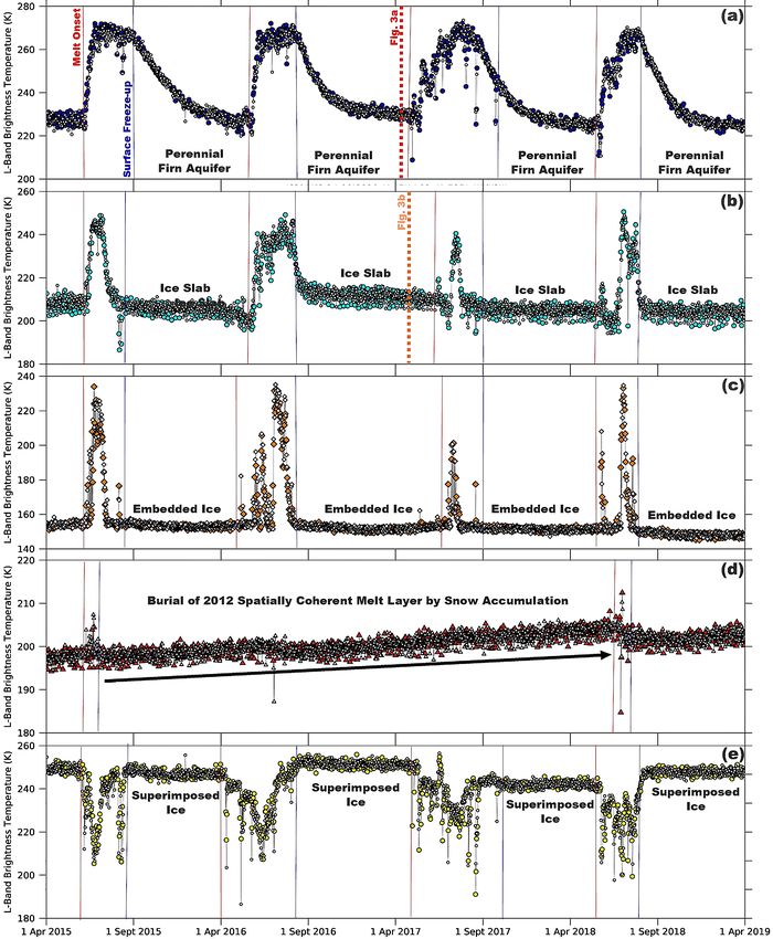
2.3.1 Temporal L-band signatures Over perennial firn aquifer areas (e.g., Fig. 4a, SMAP
Test Site A: 66.2115◦ N, 39.1795◦ W; 1625 m a.s.l.), maxi-
T B expresses the satellite-observed magnitude of thermal mum TVB (TV,max
B ) values are radiometrically warm during the
emission and is influenced by the microwave instrument’s melting season. Vertically percolating meltwater and gravity-
observation geometry as well as the depth- and time- driven meltwater drainage seasonally recharges perennial firn
integrated dielectric and geophysical properties of the ice aquifers at depth (Fountain and Walder, 1998). Minimum
sheet (Ulaby et al., 2014). The most significant geophys- B
TVB (TV,min ) values remain radiometrically warm during the
ical property influencing T B is the volumetric fraction of freezing season as a result of latent heat continuously re-
meltwater within the snow and firn pore space (Mätzler and leased by the slow refreezing of the deeper firn layers that are
Hüppi, 1989). During the melting season, the upper snow saturated with large volumetric fractions of meltwater (Miller
and firn layers of the percolation facies are saturated with et al., 2020). Temporal L-band signatures exhibit slow expo-
large volumetric fractions of meltwater that percolates ver- nential decreases and approach, and sometimes achieve, sta-
tically into the deeper firn layers (Benson, 1960; Humphrey ble TVB values. TVB can decrease by more than 50 K during
et al., 2012). Increases in the volumetric fraction of melt- the freezing season, which represents the descent of the up-
water result in rapid relative increases in the imaginary part per surface of stored meltwater by depths of meters to tens of
of the complex dielectric constant (Tiuiri et al., 1984). This meters beneath the ice sheet surface (Miège et al., 2016).
typically increases T B and decreases volume scattering and Over ice slab areas (e.g., Fig. 4b, SMAP Test Site B:
penetration depth. The L-band penetration depth can rapidly 66.8850◦ N, 42.7765◦ W; 1817 m a.s.l.), TV,max B values are
decrease from tens to hundreds of meters to less than a meter, typically radiometrically colder than over perennial firn
dependent on the local snow and firn conditions. During the aquifer areas during the melting season. The presence of
freezing season, surface and subsurface water-saturated snow dense low-permeability solid-ice layers reduces the snow and
and firn layers and embedded ice structures subsequently re- firn pore space available to store seasonal meltwater at depth.
freeze. Decreases in the volumetric fraction of meltwater re- Meltwater may alternatively run off ice slabs downslope to-
sult in rapid relative decreases in the imaginary part of the wards the wet snow facies. TV,minB values are also typically
complex dielectric constant. This decreases T B and increases radiometrically colder than over perennial firn aquifer areas
volume scattering and penetration depth. The L-band pene- during the freezing season as a result of the absence of melt-
tration depth increases back to tens to hundreds of meters on water stored at depth. Temporal L-band signatures exhibit
variable timescales. exponential decreases that are slightly more rapid than over
We analyze melting and freezing seasons in temporal L- perennial firn aquifer areas and often achieve stable TVB val-
band signatures exhibited in TVB time series over and near ues.
the AR- and MCoRDS-derived perennial firn aquifer and ice Over other percolation facies areas (e.g., Fig. 4c, SMAP
slab detections projected on the NH EASE-Grid 2.0 (Fig. 4 Test Site C: 66.9024◦ N, 44.7528◦ W; 2350 m a.s.l.), where
and Table 1). We project ice surface temperature observations seasonal meltwater is fully refrozen and stored exclusively
calculated using thermal infrared brightness temperature col- B
as embedded ice, TV,max values are typically radiometrically
lected by the Moderate Resolution Imaging Spectroradiome- colder than over perennial firn aquifer and ice slab areas
ter (MODIS) on the Terra and Aqua satellites (Hall et al., during the melting season. TV,minB values are also typically
2012) on the NH EASE-Grid 2.0 at a 3.125 km rSIR grid radiometrically cold during the freezing season. Temporal
cell spacing. We then derive melt onset and surface freeze- L-band signatures exhibit rapid exponential decreases and
up dates for each rSIR grid cell using the methodology de- achieve stable TVB values. However, over the highest eleva-
scribed in Miller et al. (2020). We set a threshold of ice sur- tions (> 2500 m a.s.l.) of the percolation facies approaching
face temperature > −1 ◦ C for meltwater detection (Nghiem the dry snow line, where seasonal surface melting and the
et al., 2012), consistent with the ±1 ◦ C accuracy of the ice formation of embedded ice structures is limited, TV,minB val-
surface temperature observations. For temperatures that are ues remain radiometrically warm during the freezing season.
close to 0 ◦ C, ice surface temperatures are closely compatible TVB decreases, often step responses exceeding 10 K, are a re-
with contemporaneous NOAA near-surface air temperature sult of an increase in volume scattering from newly formed
observations (Shuman et al., 2014). Melt onset and surface embedded ice structures within a spatially coherent melt
freeze-up dates are overlaid on TVB time series to partition the layer. Temporal L-band signatures that increase several K on
melting and freezing seasons. Melt onset dates typically oc- timescales of years indicate the burial of spatially coherent
cur between April and July, and surface freeze-up dates typi- melt layers formed following the 2010, 2012, 2015, and 2018
cally occur between July and September. The melting season melting seasons by snow accumulation.
increases in duration moving downslope from the dry snow Exponentially decreasing temporal L-band signatures
facies and ranges from a single day in the highest elevations transition smoothly between perennial firn aquifer, ice slab,
(> 2500 m) of the percolation facies to 150 d in the ablation and other percolation facies areas – there are no distinct tem-
The Cryosphere, 16, 103–125, 2022 https://doi.org/10.5194/tc-16-103-2022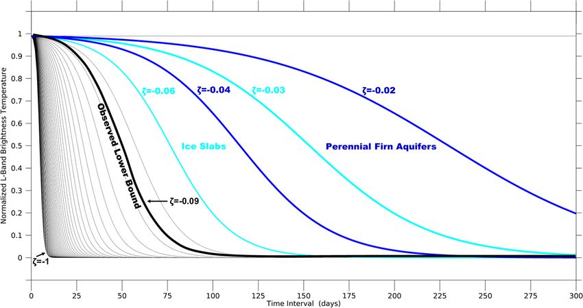
J. Z. Miller et al.: Mapping perennial firn aquifers and ice slabs                                                                         111

Figure 4. Temporal L-band signatures that alternate morning (white symbols) and evening (colored symbols) orbital pass interval enhanced-
resolution TVB generated using observations collected over the GrIS by the microwave radiometer on the SMAP satellite (Long et al., 2019)
over (a) SMAP Test Site A (blue circles; Fig. 2a), (b) B (cyan circles; Fig. 2b), (c) C (orange diamonds; Fig. 2b), (d) D (red triangles;
Fig. 2a), and (e) E (yellow circles; Fig. 2b). Melt onset (red lines) and surface freeze-up (blue lines) dates derived from thermal infrared T B
collected by MODIS on the Terra and Aqua satellites (Hall et al., 2012). AR radargram transect A-B (red dashed line; Fig. 3a) collected on
22 April 2017, and C-D (orange dashed line; Fig. 3b) collected on 5 May 2017.

poral L-band signatures that delineate boundaries between                 warm during the melting and freezing seasons. Temporal
these sub-facies. Boundary transitions between the dry snow               L-band signatures that increase on timescales of years are
facies and wet snow facies, however, are delineated above                 observed throughout the dry snow facies at elevations as
and below the percolation facies. Over the dry snow facies                high as Summit Station (3200 m a.s.l.) and indicate the burial
(e.g., Fig. 4d, SMAP Test Site D: 66.3649◦ N, 43.2115◦ W;                 of the spatially coherent melt layer formed following the
                 B
2497 m a.s.l.), TV,max      B
                       and TV,min values are radiometrically              2012 melting season (Nghiem et al., 2012) by snow accu-

https://doi.org/10.5194/tc-16-103-2022                                                               The Cryosphere, 16, 103–125, 2022
112 J. Z. Miller et al.: Mapping perennial firn aquifers and ice slabs
Table 1. MODIS-derived total number of days in the melting and freezing seasons; SMAP-derived maximum vertically polarized L-band
B
brightness temperature (TV,max ); minimum vertically polarized L-band brightness temperature (TV,min B ); timescales of exponential decrease
following the surface freeze-up date for perennial firn aquifer, ice slab, percolation facies, dry snow facies, and wet snow facies areas.
Melting season Freezing season B
TV,max B
TV,min Exponential decrease
(d) (d) (K) (K) (timescale)
Perennial firn aquifers 75–100 265–290 200–275 180–250 weeks–months
Ice slabs 60–90 275–305 170–260 130–240 days–weeks
Percolation facies 1–60 305–364 150–200 130–220 days
Dry snow facies – 365 200–240 200–240 –
Wet snow facies 90–120 245–275 230–250 230–250 –
mulation (Culberg et al., 2021). Over the wet snow facies depth and is locally dependent on embedded ice structures,
(e.g., Fig. 4e, SMAP Test Site E: 67.3454◦ N, 48.4789◦ W; spatially coherent melt layers, ice slabs, and perennial firn
1469 m a.s.l.), where seasonal meltwater is fully refrozen and aquifers. Reflectivity at depth (i.e., at the base layer–water-
B
stored as superimposed ice, TV,max values are radiometrically saturated firn layer interface) and at the ice sheet surface (i.e.,
warm during the melting season. As compared to the perco- at the water-saturated firn layer–air interface) is neglected.
lation facies, where temporal L-band signatures exhibit rapid The contribution from each layer is individually calculated.
increases following melt onset, temporal L-band signatures The two-layer L-band brightness temperature model is
reverse and exhibit rapid decreases. These reversals are a re- represented analytically by
sult of high reflectivity and attenuation at the fully water sat-
urated snow layer and/or at the wet rough superimposed ice– TV,B max = T (1 − e−κe d sec θ ) + TV,B min e−κe d sec θ , (1)
air interface. Meltwater runs off superimposed ice downslope
B B
where TV,max is the maximum vertically polarized L-band
towards the ablation facies. TV,min values remain radiometri-
cally warm during the freezing season. Temporal L-band sig- brightness temperature at the ice sheet surface and represents
natures exhibit rapid increases and achieve stable TVB values. emission from the maximum seasonal volumetric fraction of
B
meltwater stored within the water-saturated firn layer. TV,min
2.3.2 Two-layer L-band brightness temperature model is the minimum vertically polarized L-band brightness tem-
perature emitted from the base layer. T is the physical tem-
Based on our analysis of TV,maxB B
and TV,min in temporal L- perature of the water-saturated firn layer, θ is the transmis-
band signatures over the percolation facies (Sect. 2.3.1), we sion angle, κe is the extinction coefficient, and d is depth.
derive a firn saturation parameter using a simple two-layer We invert Eq. (1) and solve for the firn saturation parame-
L-band brightness temperature model (Ashcraft and Long, ter (ξ )
2006). The firn saturation parameter is similar to the “melt !
B
TV,max −T
intensity” parameter derived in Hicks and Long (2011) that
uses enhanced-resolution vertically polarized Ku-band radar ξ = ln B
cos θ , (2)
TV,min −T
backscatter imagery (2003) collected by the SeaWinds radar
scatterometer that was flown in tandem on NASA’s Quick where ξ = κe d. The maximum vertically polarized L-band
Scatterometer (QuikSCAT) satellite (Tsai et al., 2000) and brightness temperature asymptotically approaches the phys-
JAXA’s Advanced Earth Observing Satellite 2 (ADEOS-II) ical temperature of the water-saturated firn layer as the ex-
(Freilich et al., 1994). We use the firn saturation parameter to tinction coefficient and the depth of the water-saturated firn
estimate the maximum seasonal volumetric fraction of melt- layer increases. For simplicity, we follow Jezek et al. (2015)
water within the saturated upper snow and firn layers of the and define the extinction coefficient as the sum of the Raleigh
B
percolation facies using TV,max B
and TV,min values extracted scattering coefficient (κs ) and the absorption coefficient (κa ).
B
from TV time series. We calculate the firn saturation parame- This assumes scattering from snow grains, which are small
ter for each rSIR grid cell within the ice-masked extent of the (millimeter scale) relative to the L-band wavelength (21 cm),
GrIS as part of our adapted empirical algorithm (Sect. 2.3.4). and neglects Mie scattering from large (centimeter scale) em-
We assume a base layer underlying a water-saturated firn bedded ice structures. However, for water-saturated firn, ab-
layer with a given depth and volumetric fraction of meltwa- sorption dominates over scattering, and increases in the ex-
ter. Each of the layers is homogenous. The ice sheet is dis- tinction coefficient are controlled by the volumetric fraction
cretely layered to calculate TVB at an oblique incidence angle of meltwater (mv ).
(Eq. 1). Emission from the base layer is a function of both We assume that thicker water-saturated firn layers with
the macroscopic roughness and the dielectric properties of larger volumetric fractions of meltwater generate higher firn
the layer. It occurs in conjunction with volume scattering at saturation parameter values. However, the thickness of the
The Cryosphere, 16, 103–125, 2022 https://doi.org/10.5194/tc-16-103-2022J. Z. Miller et al.: Mapping perennial firn aquifers and ice slabs 113
et al., 2020) to also map the extent of ice slab areas. The
empirical algorithm is derived from the continuous logistic
model, which is based on a differential equation that models
the decrease in physical systems as a function of time using
a set of sigmoidal curves. These curves begin at a maximum
value with an initial interval of decrease that is approximately
exponential. Then, as the function approaches its minimum
value, the decrease slows to approximately linear. Finally, as
the function asymptotically reaches its minimum value, the
decrease exponentially tails off and achieves stable values.
We use the continuous logistic model to parametrize the re-
freezing rate within the water-saturated upper snow and firn
layers of the percolation facies using TVB time series that are
B
partitioned using TV,max B
and TV,min values. We calculate the
refreezing rate for each rSIR grid cell within the percola-
tion facies extent as part of our adapted empirical algorithm
(Sect. 2.3.4).
The continuous logistic model is described by a differen-
tial equation known as the logistic equation
dx
= ζ x(1 − x) (3)
dt
that has the solution
1
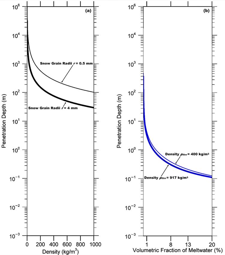
Figure 5. Theoretical L-band penetration depths for a uniform x(t) = , (4)
1
layer of (a) refrozen and (b) water-saturated firn. Penetration depths 1 + xo − 1 e−ζ t
(1/(κs + κa )) are calculated as a function of the Raleigh scattering
where xo is the function’s initial value, ζ is the function’s
coefficient (κs ; Eq. 8) and the absorption coefficient (κa ; Eq. 10).
The complex dielectric constant is calculated using the empirically
exponential rate of decrease, and t is time. The function x(t)
derived models described in Tiuri et al. (1984). Refrozen firn pene- is also known as the sigmoid function. We use the sigmoid
tration depths are calculated as a function of firn density (ρfirn ), and function to model the exponentially decreasing temporal L-
the curves are plotted for snow grain radii (r) set to r = 0.5 mm (up- band signatures observed over the percolation facies as a set
per curve) and r = 4 mm (lower curve). Water-saturated firn pene- of decreasing sigmoidal curves.
tration depths are calculated as a function of the volumetric fraction We first normalize TVB time series for each rSIR grid cell
of meltwater (mv ), and the curves are plotted for firn density set
to ρfirn = 400 kg m−3 (upper curve) and ρfirn = 917 kg m−3 (lower B
TVB (t) − TV,min
B
TV,N (t) = B B
, (5)
curve). Given the complexity of modeling embedded ice structures, TV,max − TV,min
they are excluded from the penetration depth calculation. Increases
B
where TV,min is the minimum vertically polarized L-band
in the volumetric fraction of embedded ice within the firn will result
in an increase in volume scattering, which will decrease and com- B
brightness temperature, and TV,max is the maximum vertically
press the distance between the penetration depth curves for both polarized L-band brightness temperature. We then apply the
refrozen and water-saturated firn.
sigmoid fit
B 1
TV,N (t ∈ [tmax , tmin ]) = . (6)
water-saturated firn layer is limited by the L-band penetration 1
1+ B (t
TV,N
− 1 e−ζ t
max )
depth. Theoretical L-band penetration depths calculated for a
water-saturated firn layer range from between 10 m for small B (t ∈ [t
TV,N max , tmin ]) is the normalized vertically polarized
volumetric fractions of meltwater (mv < 1 %) and 1 cm for L-band brightness temperature on the time interval t ∈
large volumetric fractions of meltwater (mv = 20 %) (Fig. 5). [tmax , tmin ], where tmax is the time the function achieves a
Large volumetric fractions of meltwater result in high reflec- maximum value, and tmin is the time the function achieves a
tivity and attenuation at the water-saturated firn layer–air in- minimum value. The initial normalized vertically polarized
terface and a radiometrically cold firn layer. L-band brightness temperature (TV,N B (t
max )) is the function’s
maximum value. The final normalized vertically polarized
2.3.3 Continuous logistic model L-band brightness temperature (TV,N B (t
min )) is the function’s
minimum value. The function’s exponential rate of decrease
We adapt our previously developed empirical algorithm to represents the refreezing rate parameter (ζ ). An example set
map the extent of Greenland’s perennial firn aquifers (Miller of simulated sigmoidal curves is shown in Fig. 6.
https://doi.org/10.5194/tc-16-103-2022 The Cryosphere, 16, 103–125, 2022114 J. Z. Miller et al.: Mapping perennial firn aquifers and ice slabs
Figure 6. Example set of simulated sigmoidal curves that represent our model of the exponentially decreasing temporal L-band signatures
predicted over the percolation facies. The initial normalized vertically polarized L-band brightness temperature was fixed at a value of
B (t
TV,N max ) = 0.99, and the time interval was set to a value of t ∈ [tmax , tmin ] = 300 observations. The refreezing rate parameter was set to
values between ζ = [−1, 0] incremented by steps of 0.02. The blue lines correspond to the interval ζ ∈ [−0.04, −0.02] and produce curves
similar to those observed over perennial firn aquifer areas. The cyan lines correspond to the interval ζ ∈ [−0.06, −0.03] and produce curves
similar to those observed over ice slab areas. The black line is the observed lower bound (ζ = −0.09) of the refreezing rate parameter of
partitioned TVB time series iteratively fit to the sigmoid function (Sect. 2.3.4).
2.3.4 SMAP-derived extent mapping and firn density estimates are consistent with measurements
within the upper snow and firn layers of the percolation facies
Our adapted empirical algorithm is implemented in two of southeastern Greenland at the Helheim Glacier field site
steps: (1) mapping the extent of the percolation facies us- (Fig. 2a, blue circle), where in situ perennial firn aquifer mea-
ing the firn saturation parameter derived from the simple surements have recently been collected (Miller et al., 2017).
two-layer L-band brightness temperature model (Sect. 2.3.2) We calculate the absorption coefficient (κa ) in Eq. (7) us-
and (2) mapping the extent of perennial firn aquifer and ice ing
slab areas over the percolation facies using the continuous √
logistic model (Sect. 2.3.3) we calibrate using airborne ice- κa = −2ko I εr , (10)
penetrating radar surveys (Sect. 2.2). where I{ } represents the imaginary part. We calculate the
Using Eq. (2), we first set a threshold for the firn saturation complex dielectric constant of the water-saturated firn layer
parameter (ξT ) defined by the relationship in Eqs. (8) and (10) using the empirically derived mod-
ξT = (κs + κa )d ≤ ξ . (7) els described in Tiuri et al. (1984). We set the volumetric
fraction of meltwater to mv = 1 %. We set the depth of the
We calculate the Raleigh scattering coefficient (κs ) in water-saturated firn layer in Eq. (7) to d = 1 m. These val-
Eq. (7) using ues are consistent with typical lower frequency (e.g., 37,
8 εr − 1 2 13.4, 19 GHz) passive (e.g., Mote et al., 1995; Abdalati and
κs = Nd ko4 r 6 , (8) Steffen, 1997; Ashcraft and Long, 2006) and active (e.g.,
3 εr + 2
Hicks and Long, 2011) microwave algorithms used to de-
where Nd is the particle density, ko is the wave number of tect seasonal surface melting over the GrIS. Using the re-
the background medium of air, r is the snow grain radius set sults of Eqs. (7–10), we calculate the firn saturation parame-
to r = 2 mm, and εr is the complex dielectric constant. The ter threshold to be ξT = 0.1.
particle density is defined by The first step in our adapted empirical algorithm is to
ρfirn 1 map the extent of the percolation facies. For each rSIR grid
Nd = , (9) cell within the ice-masked extent of the GrIS, we smooth
ρice 43 π r 3
the corresponding TVB time series using a 14-observation
where ρfirn is firn density set to ρfirn = 400 kg m−3 , and ρice (1 week) moving window. We extract the minimum verti-
is ice density set to ρice = 917 kg m−3 . Our grain radius cally polarized L-band brightness temperature (TV,minB ) and
The Cryosphere, 16, 103–125, 2022 https://doi.org/10.5194/tc-16-103-2022J. Z. Miller et al.: Mapping perennial firn aquifers and ice slabs 115
the maximum vertically polarized L-band brightness temper- which simplifies our adapted empirical algorithm. Another
B
ature (TV,max ). We set the physical temperature of the water- advantage is that unlike T B collected at shorter-wavelength
saturated firn layer to T = 273.15 K and the transmission an- thermal infrared frequencies (e.g., MODIS), T B collected at
gle to θ = 40◦ . We then calculate the firn saturation parame- longer-wavelength microwave frequencies (e.g., SMAP) is
ter (ξ ) using Eq. (2). If the calculated firn saturation parame- not sensitive to clouds, which eliminates observational gaps
ter exceeds the firn saturation parameter threshold, the rSIR and cloud contamination and provides more accurate time
grid cell is converted to a binary parameter to map the total series partitioning and more robust curve fitting.
extent of the percolation facies. We calibrate our adapted empirical algorithm using the
We note that smoothing TVB time series will mask brief AR- and MCoRDS-derived perennial firn aquifer and ice slab
low-intensity seasonal surface melting that occurs in the detections projected on the NH EASE-Grid 2.0. For each
high-elevation (> 2500 m) percolation facies, where sea- rSIR grid cell with at least one detection, we extract the
sonal meltwater is rapidly refrozen within the colder snow correlated maximum vertically polarized L-band brightness
and firn layers (e.g., Fig. 4d). Thus, the calculated firn sat- B
temperature (TV,max ), the minimum vertically polarized L-
uration parameter will not exceed the firn saturation param- band brightness temperature (TV,minB ), the firn saturation pa-
eter threshold, and these rSIR grid cells are excluded from rameter (ξ ), and the refreezing rate parameter (ζ ). For each
the algorithm. The exclusion of rSIR grid cells in the high- of the extracted calibration parameters, we calculate the stan-
elevation percolation facies is not expected to have a signifi- dard deviation (σ ). Thresholds of ±2σ are set in an attempt
cant impact on our results as our algorithm targets rSIR grid to eliminate peripheral rSIR grid cells near the ice sheet edge
cells in areas that experience intense seasonal surface melt- and near the boundaries of each sub-facies, where L-band
ing. The exclusion of rSIR grid cells may slightly underesti- emission can be influenced by morphological features, such
mate the mapped percolation facies extent. as crevasses, and superimposed and glacial ice, and spatially
The second step in our adapted empirical algorithm is integrated with emission from rock, land, the ocean, and ad-
to map the extent of perennial firn aquifer and ice slab jacent percolation facies and wet snow facies areas. The cali-
areas over the percolation facies. For each rSIR grid cell bration parameter intervals are given in Table 2. We apply the
within the mapped percolation facies extent, we normalize calibration to each rSIR grid cell within the percolation facies
the corresponding TVB time series (TV,N B (t)) using Eq. (5).
extent. If the extracted calibration parameters are within the
We then extract the initial normalized vertically polarized intervals, the rSIR grid cell is converted to a binary parameter
L-band brightness temperature (TV,N B (t
max )) and the final to map the total extent of each of these sub-facies.
normalized vertically polarized L-band brightness tempera- Miller et al. (2020) cited significant uncertainty in the
ture (TV,NB (t B
min )) and partition TV,N (t) on the time interval SMAP-derived perennial firn aquifer extent as a result of
B
t ∈ [tmax , tmin ]. We smooth TV,N (t ∈ [tmax , tmin ]) using a 56- the lack of a distinct temporal L-band signature delineating
observation (4 week) moving window. The sigmoid fit is then the boundary between perennial firn aquifer areas and ad-
iteratively applied using Eq. (6). Smoothing reduces the chi- jacent percolation facies areas. In this study, similar uncer-
B (t ∈ [t
squared error statistic when fitting TV,N max , tmin ]) to tainty exists in the SMAP-derived perennial firn aquifer and
the sigmoid function. We fix the initial normalized vertically ice slab extents. This uncertainty could, at least in part, be a
polarized L-band brightness temperature at TV,N B (t result of the rSIR algorithm. An rSIR grid cell corresponds to
max ) =
0.99, which provides a uniform parameter space in which the the weighted average of T B over SMAP’s antenna footprint
refreezing rate parameter (ζ ) can be analyzed. Variability in (Long et al., 2019). The weighting is the grid cell’s spatial
B (t
TV,N max ) is controlled by the volumetric fraction of meltwa- response function (SRF), which is approximately 18 km (i.e.,
ter within the upper snow and firn layers of the percolation the effective resolution) in diameter. The SRF is centered on
facies and is accounted for in the firn saturation parameter the rSIR grid cell. Since the effective resolution (i.e., the size
(ξ ), which is analyzed separately. TV,N B (t ∈ [t
max , tmin ]) val- of the 3 dB contour of the SRF) is greater than the rSIR grid
ues iteratively fit to the sigmoid function converge quickly cell spacing, the rSIR grid cell SRF’s overlap and the T B val-
(i.e., algorithm iterations I ∈ [5, 15]), and observations are a ues are not statistically independent. This uncertainty, how-
good fit (i.e., chi-squared error statistic is χ 2 ∈ [0, 0.1]). ever, could also have a geophysical basis, as it is unlikely that
Using the SMAP-derived TV,N B (t B
max ) and TV,N (tmin ), rather the boundaries between sub-facies as well as between facies
than the MODIS-derived initial normalized vertically polar- are distinct. The thickness of the water-saturated firn layer
ized L-band brightness temperature at the surface freeze- or ice slab may thin and taper off at the periphery, and sub-
up date (TV,N B (t )), and final normalized vertically polar- facies and facies may become spatially scattered and merge
sfu
ized L-band brightness temperature at the melt onset date together.
B (t )) that were used in the empirical algorithm de-
(TV,N The limited extent (AR, 15 m × 20 m; MCoRDS, 14 m ×
mo
scribed in Miller et al. (2020), has several advantages. The 40 m) of the airborne ice-penetrating radar surveys as com-
key advantage of this approach is that maps can be gen- pared to the rSIR grid cell extent (3.125 km) and the effective
erated using T B imagery collected from a single satellite, resolution of the SMAP enhanced-resolution TVB imagery is
https://doi.org/10.5194/tc-16-103-2022 The Cryosphere, 16, 103–125, 2022You can also read