Analysis algorithm for sky type and ice halo recognition in all-sky images - Atmos. Meas. Tech
←
→
Page content transcription
If your browser does not render page correctly, please read the page content below

Atmos. Meas. Tech., 12, 4241–4259, 2019
https://doi.org/10.5194/amt-12-4241-2019
© Author(s) 2019. This work is distributed under
the Creative Commons Attribution 4.0 License.

Analysis algorithm for sky type and ice halo recognition
in all-sky images
Sylke Boyd, Stephen Sorenson, Shelby Richard, Michelle King, and Morton Greenslit
Division for Science and Mathematics, University of Minnesota Morris, 500 E 4th Street, Morris, MN, USA

Correspondence: Sylke Boyd (sboyd@morris.umn.edu)

Received: 15 November 2018 – Discussion started: 7 January 2019
Revised: 14 June 2019 – Accepted: 10 July 2019 – Published: 6 August 2019

Abstract. Halo displays, in particular the 22◦ halo, have been     1   Introduction
captured in long time series of images obtained from total
sky imagers (TSIs) at various Atmospheric Radiation Mea-           Modeling and predicting the Earth’s climate is a challenge
surement (ARM) sites. Halo displays form if smooth-faced           for physical science, even more so in light of the already
hexagonal ice crystals are present in the optical path. We de-     observable changes in Earth’s climate system (Fasullo and
scribe an image analysis algorithm for long time series of         Balmaseda, 2014; Fasullo et al., 2016; IPCC, 2013, 2014).
TSI images which scores images with respect to the pres-           Global circulation models (GCMs) describe the atmosphere
ence of 22◦ halos. Each image is assigned an ice halo score        in terms of a radiative dynamic equilibrium. The Earth re-
(IHS) for 22◦ halos, as well as a photographic sky type (PST),     ceives solar shortwave (SW) radiation and discards energy
which differentiates cirrostratus (PST-CS), partially cloudy       back into space in the form of terrestrial long-wave (LW)
(PST-PCL), cloudy (PST-CLD), or clear (PST-CLR) within             radiation. The radiation balance of the Earth has been sub-
a near-solar image analysis area. The color-resolved radial        ject to much study and discussion (Trenberth et al., 2014;
brightness behavior of the near-solar region is used to de-        Fasullo and Kiehl, 2009; Kandel and Viollier, 2010; Tren-
fine the discriminant properties used to classify photographic     berth et al., 2015). Global circulation models describe the in-
sky type and assign an ice halo score. The scoring is based        fluence of various parts of the Earth system in terms of radia-
on the tools of multivariate Gaussian analysis applied to a        tive forcing factors (Kandel and Viollier, 2010; Kollias et al.,
standardized sun-centered image produced from the raw TSI          2007). Clouds may restrict the SW flux reaching the surface,
image, following a series of calibrations, rotation, and co-       but they also influence the LW emissions back into space.
ordinate transformation. The algorithm is trained based on         While low stratus and cumulus clouds exhibit a net negative
a training set for each class of images. We present test re-       radiative forcing, high cirroform clouds are more varied in
sults on halo observations and photographic sky type for the       their radiative response, varying between negative and posi-
first 4 months of the year 2018, for TSI images obtained           tive forcing depending on time of day, season, and geograph-
at the Southern Great Plains (SGP) ARM site. A detailed            ical location (Campbell et al., 2016). The Fifth Assessment
comparison of visual and algorithm scores for the month of         Report from the IPCC in 2013 (IPCC, 2013) identified ice
March 2018 shows that the algorithm is about 90 % reliable         and mixed clouds as major contributors to the low confidence
in discriminating the four photographic sky types and iden-        level into the aerosol and cloud radiative forcing. The uncer-
tifies 86 % of all visual halos correctly. Numerous instances      tainty in the aerosol and cloud forcing has implications for
of halo appearances were identified for the period January         the confidence in and for the variance of the predictions of
through April 2018, with persistence times between 5 and           global circulation models (Fu et al., 2002; Trenberth et al.,
220 min. Varying by month, we found that between 9 % and           2015). Closing the radiation budget of the Earth hinges on re-
22 % of cirrostratus skies exhibited a full or partial 22◦ halo.   liable cloud data (Hammer et al., 2017; Schwartz et al., 2014;
                                                                   Knobelspiesse et al., 2015; Waliser et al., 2009). Tradition-
                                                                   ally, cloud radiative forcing is modeled using a cloud frac-
                                                                   tion based on sky images (Kennedy et al., 2016; Kollias et

Published by Copernicus Publications on behalf of the European Geosciences Union.
4242                                                  S. Boyd et al.: Analysis algorithm for sky type and ice halo recognition

al., 2007; Schwartz et al., 2014). Cirrostratus clouds, lacking    the University of Minnesota Morris, using an all-sky camera,
sharp outlines, pose a challenge to this approach (Schwartz        through a 5-month period in 2015, and found an abundance
et al., 2014). The uncertainty about the role of cirrus in the     of halo features.
global energy balance has been attributed to limited obser-           There are a few studies pursuing a similar line of inquiry
vational data concerning their temporal and spatial distribu-      (Forster et al., 2017; Sassen et al., 2003). The study by Sassen
tion, as well as their microphysics (Waliser et al., 2009). Cir-   et al. (2003) showed a prevalence of the 22◦ halo, full in 6 %
roform clouds, at altitudes between 5000 and 12 000 m, are         and partial in 37.3 % of cirrus periods, based on a 10-year
effective LW absorbers. Cloud particle sizes can range from        photographic and lidar record of midlatitude cirrus clouds,
a few microns to even centimeter sizes (Cziczo and Froyd,          also providing data on parhelia, upper tangent arcs, and other
2014; Heymsfield et al., 2013). Methods to probe cirrus cloud      halo display features, as well as coronas. The photographic
particles directly involve aircraft sampling (Heymsfield et al.,   record was taken in Utah and based on 20 min observation
2013) and mountainside observations (Hammer et al., 2015).         intervals; cirrus identification was supported by lidar. The
Ground- and satellite-based indirect radar and lidar measure-      authors found an interesting variability in halo displays, re-
ments (Hammer et al., 2015; Hong et al., 2016; Tian et al.,        lated to geographical air mass origin, and suggest that optical
2010) give reliable data on altitudes, optical depths, and par-    displays may serve as tracers of the cloud microphysics in-
ticle phase. Even combined, these methods leave gaps in the        volved. Forster et al. (2017) used a sun-tracking camera sys-
data for spatial and temporal composition of ice clouds. The       tem to observe halo display details over the course of several
analysis of halo displays as captured by long-term total sky       months in Munich, Germany, and a multiweek campaign in
imagers may provide further insight and allow one to close         the Netherlands in November 2014. A carefully calibrated
some of the gaps.                                                  camera system provided high-resolution images, for which
   Optical scattering behavior is influenced by the types of       a halo detection algorithm was presented, based on a deci-
ice particles, which may be present in very many forms, in-        sion tree and random forest classifiers. Ceilometer data and
cluding crystalline hexagonal habits in the form of plates,        cloud temperature measurements from radiosonde measure-
pencils and prisms, hollow columns, bullets and bullet             ments were used to identify cirrus clouds. The authors report
rosettes, and amorphous ice pellets, fragments, rimed crys-        25 % of all cirrus clouds also produced halo displays, in par-
tals, and others (Bailey and Hallett, 2009; Baran, 2009; Yang      ticular in the sky segments located above the sun. The frac-
et al., 2015). Only ice particles with a simple crystal habit      tion of smooth crystals necessary for halo display appearance
and smooth surfaces can lead to halo displays (Um and Mc-          is at a minimum 10 % for columns, and 40 % for plates, based
Farquhar, 2015; van Diedenhoven, 2014). Usually, this will         on an analysis of scattering phase functions for single scatter-
be the hexagonal prism habit, which we can find in plates,         ing events (van Diedenhoven, 2014). While this establishes a
columns, bullet rosettes, pencil crystals, etc. If no preferred    lower boundary, it is correct to say that the observability of
orientation exists, a clear telltale sign for their presence is    a halo display allows one to conclude that smooth crystalline
the 22◦ halo around a light source in the sky, usually sun         ice particles are present and single scattering events domi-
or moon. More symmetry in the particle orientations will           nate. The consideration of the percentage of cirrus clouds that
add additional halo display features such as parhelia, upper       display optical halo features allows therefore, upon further
tangent arc, circumscribed halo, and others (Greenler, 1980;       study, inferences about the microphysical properties of the
Tape and Moilanen, 2006). As shown in theoretical stud-            cloud. This raises interest in examining existing long-term
ies (van Diedenhoven, 2014; Yang et al., 2015), halos form         records of sky images.
in particular if the ice crystals exhibit smooth surfaces. In         Long-term records of sky images have been accumulated
that case, the forward-scattered intensity is much more pro-       in multiple global sites. The Office of Science in the US De-
nounced as in cases of rough surfaces, even if a crystal habit     partment of Energy has maintained Atmospheric Radiation
is present. If many of the ice particles are amorphous in na-      Measurement (ARM) sites. These sites, among other instru-
ture, or did not form under conditions of crystal growth –         ments, contain a total sky imager (TSI) and have produced
for example by freezing from supercooled droplets, or by           multiyear records of sky images. In this paper, we introduce a
riming – the forward scattering pattern will be weaker and         computational method to analyze these long-term records for
similar to what we see for liquid droplets: a white scatter-       the presence of halo displays in the images. We are introduc-
ing disk surrounding the sun, but no halo. In turn, roughness      ing an algorithm to analyze long sequences of TSI images.
and asymmetry of ice crystals influence the magnitude of           The algorithm produces a time record of near-solar photo-
backscattered solar radiation, thus influencing the radiative      graphic sky type (PST), differentiated as cirrostratus (PST-
effect of cirrus clouds (van Diedenhoven, 2016). If the parti-     CS), partly cloudy (PST-PCL), cloudy (PST-CLD), and clear
cles in the cirroform cloud are very small, e.g., a few microns    (PST-CLR) sky types, as well as assigns an ice halo score
(Sassen, 1991), diffraction will lead to a corona. We believe      (IHS). The resolution and distortion of the TSI images re-
that a systematic observation of the optical scattering proper-    strict the halo search to the common 22◦ halo. Other halo
ties adds information to our data on cirrus microphysics and       features, such as parhelia, can occasionally be seen in a TSI
cirrus radiative properties. The authors observed the sky at       image but often are too weak or too small to reliably discrimi-

Atmos. Meas. Tech., 12, 4241–4259, 2019                                              www.atmos-meas-tech.net/12/4241/2019/
S. Boyd et al.: Analysis algorithm for sky type and ice halo recognition 4243
nate them from clouds and or 22◦ halos. If present they would in Table 2. The 80 sample images were used to develop the
be classified by this algorithm as part of a 22◦ halo. Coronas algorithm and define a suitable set of characteristic proper-
are obscured by the shadow strip and often also by overexpo- ties for PST score (PSTS) and IHS. This set will be referred
sure in the near-solar area of the image. The algorithm offers to as seed images since they also initialize the master table
an efficient method of finding 22◦ halo incidences, full or described below.
partial. Since ARM sites also have collected records of li-
dar and radiometric data, the TSI halo algorithm is intended
to be compared to other instrumental records from the same 3 Algorithm
locations and times. This will be addressed in future work.
3.1 Goal and strategy
Section 1 describes the TSI data used in this work. Sec-
tion 2 presents the details of the image analysis algorithm, The algorithm aims to process very large numbers of images
including subsections on algorithm goals, image preparation, and return information about the presence of 22◦ halos, as
and sky type and halo scoring. Section 3 applies the algo- well as the general sky conditions. The program is written
rithm to the TSI data record of the first 4 months of 2018 and in C++ and uses the OpenCV library for image process-
examines the effectiveness and types of data available for this ing. If given a list of image directories, the algorithm pro-
interval. Summary and outlook are given in Sect. 4. ceeds to sequentially import, process, and score TSI images
compared to training sets gleaned from representative im-
ages for each scored class. We define four classes of photo-
2 TSI images graphic sky types, listed in Table 2, and a halo class. The fac-
tors that determine these choices are discussed in Sect. 2.3.1
Images used in this paper were obtained from Atmospheric and 2.3.3. The algorithm assigns a numeric photographic sky
Research Measurement (ARM) Climate Research Facilities type score (PSTS) and a numeric ice halo score. For all im-
in three different locations: Eastern North Atlantic (ENA) age classes, sets of discriminant image properties have been
Graciosa Island, Azores, Portugal; North Slope of Alaska defined which differ between 10 distinct properties for PST
(NSA) Central Facility, Barrow, AK; and Southern Great classes and 31 distinct properties for the halo class.
Plains (SGP) Central Facility, Lamont, OK (ARM, 2000). Multivariate analysis is one of the standard methods in im-
The ranges and dates vary by location, as listed in Table 1. age analysis, applied in a wide variety of problems. Numer-
The images were taken with total sky imagers, which consist ous text books provide introductions to this method in a the-
of a camera directed downward toward a convex mirror to oretical background (Harris, 1975; Gnanadesikan, 1977) as
view the whole sky from zenith to horizon. A sun-tracking well as in an application-oriented manner (Alpaydin, 2014;
shadow band is used to block the sun, which covers a strip of Flury, 1988). A set of Np discriminant properties of the im-
sky from zenith to horizon. Images were recorded every 30 s. age is chosen, selected to be characteristic for a particular sky
The longest series was taken at the Southern Great Plains type or the presence of a halo. Let this set of properties be the
location, reaching back to July 2000. The images, in JPEG observation vector
format, have been taken continuously during daytime. Aside N
from nighttime and polar night, there are some additional X = {xi }i p . (1)
gaps in the data, perhaps due to instrument failure or other
For each class, a training set is created. The training set
causes. Camera quality, exposure, mirror reflectance, image
is a set of Nt observation vectors for images that have been
resolution, and image orientation varies over time as well as
visually assigned to the class. A training set defines an el-
by location. For example, an image from SGP taken in 2018
lipsoidal centroid in the property space of X, centered at the
has a size of 488 pixels by 640 pixels. The short dimension
mean observation vector
limits the radius of the view circle to at most 240 pixels.
pN
A pixel close to the center of the view circle corresponds M = {µi }i=1 , (2)
to an angular sky section 2.8◦ wide and 0.24◦ tall. At SGP, 1 XNt
the solar position never reaches this point. Close to the hori- µi = x .
k=1 ik
(3)
Nt
zon, 1-pixel averages a sky section that is 0.24◦ wide and
1.24◦ tall. Best resolution is achieved at zenith angle 45◦ , in The centroid’s extent is described by the Np × Np covari-
which case every pixel represents a sky region of 0.33◦ by ance matrix
0.33◦ . The perspective distortion is largest for sky segments
σ11 σ12 . . .
close to the horizon due to perspective distortions of the sky. 6 = (X − M) (X − M)T = σ21 σ22 . . . , (4)
We used a sampling of 80 images taken from across the TSI ... ... ...
record and across all available years to initiate the training
set (ARM, 2000). This included images visually classified with elements
from the images as photographic sky types CS, PCL, CLD, 1 XNt
CLR, and halo-bearing. Descriptions of the PST are provided σij = x x − µi µj .
k=1 ik j k
(5)
Nt
www.atmos-meas-tech.net/12/4241/2019/ Atmos. Meas. Tech., 12, 4241–4259, 20194244 S. Boyd et al.: Analysis algorithm for sky type and ice halo recognition
Table 1. TSI data set properties. Seed images for the algorithm were taken from all three locations. Data source: ARM (2000).
Location Dates and times (UTC) Image interval Resolution (pixels)
Southern Great Plains 2 Jul 2000 0:35:00 15 Aug 2011 01:17:30 30 s 288 × 352
36◦ 360 1800 N, 97◦ 290 600 W 15 Aug 2011 22:17:30 19 Apr 2018 01:02:00 30 s 480 × 640
North Slope of Alaska 25 Apr 2006 21:44:00 2 Nov 2010 21:31:00 30 s 288 × 352
71◦ 190 22.800 N, 156◦ 360 32.400 W 9 Mar 2011 01:08:30 11 Apr 2018 18:59:30 30 s 480 × 640
Eastern North Atlantic 1 Oct 2013 08:13:00 28 May 2018 21:04:00 30 s 480 × 640
39◦ 50 29.7600 N, 28◦ 10 32.5200 W
Table 2. Descriptions of the photographic sky types (PST).
Sky type Visual description
Cirrostratus PST-CS Muted blue, no sharp cloud outlines; solar position clearly visible, bright scattering disk
or halo may be present; changes are gradual and slow (several minutes).
Partly cloudy PST-PCL Variable sky with sharply outlined stratocumulus or altocumulus; variations between sky
quadrants; sun may be obscured; changes are abrupt and fast (less than 2 min).
Cloudy PST-CLD Sun is obscured; low brightness; low blue intensity values; stratus, nimbostratus, altostra-
tus, or cumulonimbus; changes occur slowly (order of hours).
Clear PST-CLR Blue, cloud-free sky; sun clearly visible and no bright scattering disk around it; changes
are slow (order of hours).
No data N/A This may occur at low sun positions for the bottom quadrants of the LSM, or due to
overexposure in the near-solar region of the image; it is the default at night.
The observation vector of any further image X0 will then be needs to import M and 6 −1 for each class once at the start
referenced with M and 6 in the form of a multivariate nor- of the analysis run. The training sets for each class of images
mal distribution: are started using the set of 80 images described in Sect. 1 and
are expanded as needed. This allows one to continually train
1 T
the algorithm toward improvement of scoring. This basic al-
F = C0 exp − X 0 − M 6 −1 X0 − M ,
(6)
2 gorithm structure is used on a standardized local sky map,
described in Sect. 2.2. The details of PSTS and IHS will be
in which the quadratic form in the exponent is known as the
described separately below. The code and accessories can be
square of the Mahalanobis distance in property space. The
accessed at a GitHub repository (Boyd et al., 2018).
closer an image places to the centroid of a class, the higher
its score Eq. (6) will be. The Mahalanobis distance is ex-
pressed in units of standard deviations, eliminating the influ- 3.2 Image preparations and local sky map (LSM)
ence of the units of the discriminant properties and the need
for weights. It is interesting to note that the average Maha-
lanobis distance for a class is equal to the number of discrim- The goal of the image preparation is to create a local sky map
inant properties. The prefactor C0 in Eq. (6) is different for (LSM) centered at the sun, in easy-to-use coordinates, after
the photographic sky type scores and the ice halo score since a minimal color calibration and after extraneous image parts
the dimensionality of the observation vectors for these two have been masked. The image preparations include the fol-
class types is different. It is chosen to place the values for F lowing steps: (1) a color correction, (2) an alignment calibra-
into a convenient number range. The value F for each class tion, (3) a removal of the perspective distortion, (4) masking
of images is akin to a continuous numerical probability that and marking of the solar position, and (5) rotation and crop
the image is located close to the centroid of this particular to create a local sky map. Some sample steps in the image
class. preparation are illustrated in Fig. 2. The figure includes the
The algorithm is outlined in Fig. 1, together with the re- original image, the image after preparation step (4), and the
spective references to this text. Both M and 6 −1 are com- LSM after preparation step (5). The two sample images in
puted a priori from the training sets via Eqs. (2) and (4). In Fig. 2 were taken at the Southern Great Plains ARM site in
order to score a time series of property vectors X, one only March and April 2018 (SGP, 2018). One of the images con-
Atmos. Meas. Tech., 12, 4241–4259, 2019 www.atmos-meas-tech.net/12/4241/2019/S. Boyd et al.: Analysis algorithm for sky type and ice halo recognition 4245
Figure 1. Flow chart of the algorithm for the analysis of TSI images.
tains a solar 22◦ halo, and the other one is a partly cloudy sky The color values represent the intensity of the color channel
without any halo indications. registered for the particular pixel, varying between 0 (no in-
Step (1) is a color correction. Both original images in tensity) and 255 (brightest possible). In a discolored series,
Fig. 2 have a slightly green tinge, which is typical for im- measurements of BGR were taken in clear-sky images (in-
ages from the TSI at this location, in particular after an in- dexed PST-CLR), and a scaling factor and weight for each
strument update in 2010. This is noticeable in particular if color channel were defined based on this information:
images are compared to earlier TSI data from the same loca-
tion, and it can become a problem for the planned analysis, βB = 1.00 with (Bref , Gref , Rref )
especially for the use of relative color values. Since the algo- Gref BCLR
βG = ×
rithm is intended for multiple TSI locations and records taken GCLR Bref = (180, 120, 85) . (7)
Rref BCLR
over a long time, including device changes, it is necessary to βR = ×
consider the fact that no two camera devices have exactly the RCLR Bref
same color response, even if of the same type (Ilie and Welch, The reference values are based on color values for clear sky
2005). The color calibration used in this algorithm is based images from the TSI records listed in Table 1. Near-zenith,
on sampling of clear-sky color channels to define weighed clear blue sky provides a reproducible color reference in all
scaling factors for a whole series of images. Every pixel in the locations. Once these color-scaling factors were deter-
a TSI image exhibits a value between 0 and 255 for each mined for a series, every image was then tinted by generating
of the three color channels blue (B), green (G), and red (R).
an average color B, G, R for a small near-zenith sky sample
www.atmos-meas-tech.net/12/4241/2019/ Atmos. Meas. Tech., 12, 4241–4259, 20194246 S. Boyd et al.: Analysis algorithm for sky type and ice halo recognition
tint, and α = 1 produces an image of a single color. This tint-
ing is minimal, and linear color behavior is a reasonable as-
sumption.
Step (2) is a stretch-and-shift process that identifies the
horizon circle. Occasionally, a slight misalignment of the
camera and mirror axis leads to an elliptical appearance of
the sky image. A calibration is necessary in such cases to
stretch the visible horizon ellipse to a circular shape and to
center the horizon circle as close to the zenith as possible.
A north–south alignment correction may also have to be ap-
plied. Both calibrations will ensure successful identification
of the solar position in the next step. These calibrations be-
come necessary if the TSI was not perfectly aligned in the
field. They need to be readjusted after any disturbances oc-
curred to the instrument, such as storms, snow, and instru-
ment maintenance. Typically, this can be once every few
months, or sometimes several times per month. It is impor-
tant to check the calibrations regularly by sampling across
the series whether the solar position was correctly identified
after calibration. In addition, the horizon circle is placed at a
zenith angle smaller than 90◦ , often between 85 and 79◦ , to
eliminate the strong view distortion close to the horizon and,
in some cases, objects present in the view. As explained ear-
lier, the zenith angle resolution per pixel exceeds 1.2◦ close
to the horizon. The information value for a solar zenith angle
(SZA) larger than 80◦ is diminished. These pixels are ex-
cluded from the analysis. Practically, this is a very thin ring
cut from the original image but does help eliminate false sig-
nals at low sun angles. The current process requires one to
find these calibrations for a small sampling of images in a
series and to then apply them to all images in the series.
Step (3) removes the perspective distortion. The projection
of the sky onto the plane of an image introduces a perspec-
tive distortion, as described in Long et al. (2006). A coordi-
nate transformation is performed to represent the sky within
the horizon circle in terms of azimuth and zenith angle. The
Figure 2. Two examples for image preparation. The left column azimuth is the same in both projections. Zenith angle θ re-
develops an image from SGP 17 April 2018 17:45:00 UTC, and lates to the radial distance r in the original image from the
the right image was taken on SGP 3 April 2018 19:09:30 UTC. (a, center of the horizon circle as r = R sin θ. While R is not de-
b) Original image; (c, d) image after color correction, distortion termined, image horizon radius RH and horizon zenith angle
removal, masking of horizon and equipment, and sun mark were
θH provide one known point to allow for proportional scal-
applied; (e, f) final local sky map with sun at center and a width of
about 80 LSM units.
ing. The coordinate transformation represents the sky circle
in a way in which radial distance from zenith sz scales with
zenith angle θ as
and applying RH
sz = × θ. (9)
sin θH
B0 = B + α βB B − B
G0 = G + α βG G − G (8) Long et al. (2006) discuss a further image distortion intro-
R0 = B + α βR R − R duced by the particulars of the optics of the system of convex
mirror and camera. The authors give an empirical correction
to each color channel and pixel, respectively, followed by a curve for the SZA transformation. This correction is small; it
simple
√ scaling to preserve the total brightness of the pixel has been omitted in this algorithm. One of the visible effects
I = B2 + G2 + R2 . For the series SGP 2018, these factors of this transformation concerns 22◦ halos: in the original TSI
were β = (0.9, 0.78, 1) and α = 0.4. The coefficient α regu- image, a halo appears as a horizontal ellipse; after the trans-
lates the strength of the tinting such that α = 0 leads to no formation it will have a shape closer to a circle.
Atmos. Meas. Tech., 12, 4241–4259, 2019 www.atmos-meas-tech.net/12/4241/2019/S. Boyd et al.: Analysis algorithm for sky type and ice halo recognition 4247
Equation (10) provides a unit transformation between
pixel positions and LSM units. For a TSI image of size
480 pixels × 640 pixels, the LSM will have a size of approx-
imately 240 pixels × 240 pixels. For the earlier, smaller TSI
images, the LSM has a size of approximately 140 pixels ×
140 pixels. The unit scaling includes the calibration choices
RH and θH ; hence, there is a slight variation in LSM side
lengths. We eliminate the influence of the LSM sizes by per-
forming all algorithm operations in standardized LSM units,
which roughly correspond to angles of 1◦ . In other words,
all LSMs are equivalent to each other in terms of their LSM
units but not in terms of pixel positions. At θ = 45◦ , the arc
length of azimuth angle φ is equivalent to the arc length
of θ of same size; however, if θ > 45◦ , the azimuth arc is
stretched, requiring an additional horizontal compression to
ensure equivalence of horizontal and vertical angular units.
The LSM is divided into quadrants, shown in Fig. 3, which
are analyzed and classified separately by the algorithm de-
scribed in the next section.
3.3 Computing photographic sky type and halo
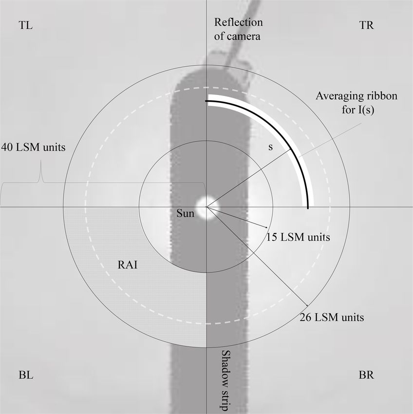
Figure 3. Layout of the local sky map (LSM). The LSM is divided properties
into four quadrants, named according to their position as TR – top
right, BR – bottom right, BL – bottom left, and TL – top left. The
3.3.1 Average radial intensity (ARI)
RAI is the radial analysis interval for which PST and IHS properties
are evaluated. The approximate position of the halo maximum is
sketched in light gray. Shadow strip and camera are excluded from Halos, as sun-centered circles, are creating a brightness sig-
analysis. nal at a scattering angle of 22◦ . We found it useful to analyze
the radial brightness I (s), with s being the radial distance
from the sun in the image plane, similar to the halo detec-
Step (4) identifies the solar position and masks nonsky de- tion algorithm by Forster et al. (2017). The term intensity
tails. The position of the sun is marked based on the geo- refers to the color values of any of the color channels and
graphical position of the TSI and the Universal Time (UTC) varies between 0 and 255. There is a physical reason for us-
of the image. Extraneous details, such as the shadow strip, ing I (s) in PST and halo assessment. The presence of scat-
the area outside the horizon circle, the camera, and the cam- tering centers in the atmosphere influences the properties of
era mount, are masked. Figure 2c and d show the image pro- sky brightness in the near-sun sky section. A very clear atmo-
duced by all these adjustments up to step (4). Since often the sphere, for example, exhibits an exponential decline, but with
position of the sun is detectable in the image, the marked sun relatively high intensity values in the blue channel due to
position serves to refine the calibrations described above. Rayleigh scattering. In the case of cirrostratus, the increased
In step (5), the standardized local sky map is created. A forward scattering of larger particles (in this case ice crys-
sketch of the layout of the LSM is provided in Fig. 3. The tals) leads to a decreased gradient of radial brightness, with
LSM provides a standard sky section, centered at the sun, more evenly distributed intensities in the red, green, and blue
oriented with the horizon at the bottom, and presented in the channels. In a partially cloudy sky, we would find sharp vari-
same units for all possible TSI images (independent on the ations in I (s), varying with color channel. An overcast sky,
resolution of the original). Units of measurement in the LSM on the other hand, may exhibit no decline in radial brightness
are closely related to angular degrees but do not match per- and will generally have low intensity values across all color
fectly due to a zenith angle dependence of the azimuth arc channels. A sketch of the LSM is given in Fig. 3. The radial
length. The LSM is generated by rotating and cropping the intensity I (s) is computed using the color intensity values of
image from step (4) to approximately within 40◦ of the sun, the image (0 to 255), separated by color channel. The LSM
with the sun at its center. is divided into four quadrants: TR represents top right, BR
The side length of the LSM in pixels scales with the pre- represents bottom right, BL represents bottom left, and TL
viously determined horizon radius RH in pixels and the cor- represents top left, analyzed separately for quadrant scores,
responding maximum zenith angle θH in ◦ as and then recombined for the image scores. The division into
quarters allows one to accommodate partial halos, low so-
RH (pixels) ◦ lar positions, and the influence of low clouds in partially ob-
wLSM (pixels) = × 40 . (10) structing the view to cirrostratus. The algorithm uses various
θH (degrees)
www.atmos-meas-tech.net/12/4241/2019/ Atmos. Meas. Tech., 12, 4241–4259, 20194248 S. Boyd et al.: Analysis algorithm for sky type and ice halo recognition
properties of I (s) to assign numeric PSTS and IHS, as de- by color channel. To set apart clear skies, the average color
tailed below. ratio (ACR) in the analysis area is computed as
The average radial intensity I (s) is computed as an aver-
age over pixels at constant radial distance s from the sun. Due B2
ACR = . (13)
to the low resolution of the LSM, and due to some noise in GR
the data, we average I (s) over a circular ribbon with a width
of 4 pixels, centered at s. Computing I (s) over a thin ribbon In Fig. 5, the PST property set is represented graphically, in-
addresses issues encountered when averaging over a circle cluding means, standard deviations, and extreme values as
in a coarse square grid, allowing continuity where otherwise observed for the completed training set. Clearly, no single
pixelation may interrupt the line of the circle. Figure 4 shows property alone will suffice to assign a PST reliably. There is
the radial intensity of the red channel (R) in the bottom right overlap in the extreme ranges. Relations between the color
quadrants of the LSMs featured in Fig. 2. Panel a includes channels are influential as well. We are using the mechanism
I (s), a linear fit, as well as the running average I 6 , plotted described in Sect. 2.1, Eqs. (1) through (6). The training sets
versus radial distance s. The running average is taken as the for each class are collected in a master table, where M and
average of I (s) over a width of 6 LSM units centered at s: 6 −1 for each PST are computed. As a new image is pro-
cessed, and its PST property vector X is computed for each
1 Xs+3 LSM units sky quadrant. Subsequently, a numeric score is computed for
I 6 (s) = I (s) . (11)
N s−3 LSM units each sky type using Eq. (6). The coefficient C0 in Eq. (6)
for the PSTS computation is chosen as 103 , which places a
The clear-sky image exhibits a lower red intensity overall
rough separator of order 1 between images that match closely
than the halo image. The halo presents as a brightness fluc-
a particular sky type and those which do not. The raw values
tuation at about 21 LSM units. The analysis of I (s) is under-
of Fimage in Eq. (6) vary greatly even between similar look-
taken in an interval between 15 and 26 LSM units, called the
ing images; hence the PSTS is computed as a relative con-
radial analysis interval (RAI). The RAI is marked in Fig. 3.
tribution between 0 % and 100 % for each sky type and each
A linear fit yields a slope and intercept value used for the
quadrant. For the PST-CS score this would mean
PSTS. We define the radial intensity deviation as
FCS
η (s) = I (s) − I 6 (s) . (12) PST_CS = × 100 % (14)
FCS + FPCL + FCLD + FCLR
Panels b in Fig. 4 show η(s) for both situations. The details
of the halo signal in η(s) contribute in particular to the com- and equivalent for all other PST classes. A single image
putation of the IHS. quadrant can carry scores of 45 % for PST-CS, 35 % for PST-
PCL, and 20 % for PST-CLD. The dominant sky type then
3.3.2 Photographic sky type (PST) is PST-CS for this quadrant, since it contributes the largest
score. The PSTS for the image is assigned as the average
The training sets for the properties of I (s) were started for over all quadrants. If the raw scores F for all PSTs were
the set of 80 seed images mentioned in Sect. 1. Twenty im- smaller than 10−8 , the quadrant is classified as N/A. It sim-
ages for each sky type were divided further by sky quadrants, ply means that its properties are not close to any of the PST
yielding between 60 and 80 property sets for each sky type to categories. Such conditions may include overexposed quad-
initiate the training sets. Some quadrants were eliminated by rants, near-horizon sun positions, a bird sitting on the mirror,
near-horizon sun positions. The training quadrants were used and other conditions that produce images very different from
to apprise the utility of I (s) in making sky type assignments, the PST sought after. Also classified as N/A are quadrants in
with focus on the radial analysis interval between 15 and 26 which the average radial intensity lies above 253 (overexpo-
LSM units. The 10 image properties used to compute the nu- sure) or contains a large fraction of horizon (bottom quad-
meric PSTS are listed in Table 3. Also listed are the compo- rants in low sun positions). A 1 d sample of sky type data is
nents of M together with their standard deviations, computed shown in Fig. 6, for 10 March 2018. The day was chosen for
from a later and more complete version of the training sets. its variability, including periods of each of the PST, as well
The 10 image properties include the slope and intercept of the as clearly visible halo periods. The central panel tracks the
line fit to I (s) for each color channel, where the slope charac- PSTS for all photographic sky types through the day, taken
terizes a general brightness gradient, and the intercept gives for all four LSM quadrants combined. It is important to note
access the overall brightness in the RAI. The line fit alone that the PST only can be representative of the section of sky
will not allow one to differentiate partially cloudy skies from near to the sun. Some of the late-day images in Fig. 6 con-
other sky types. However, the presence of sharply outlined tain quadrants that were eliminated due to overexposure. The
clouds leads to a larger variation in intensity values, even for white scattering disk around the sun near the horizon does
the same radial distance from the sun. The areal standard de- not allow for analysis, which is exemplified in the sample
viation (ASD) is an average of the standard deviation of I (s) image at 22:53:00 UTC included in Fig. 6. For large portions
for each radial distance s, averaged over all radii separated of the day, the dominant sky types have been classified as
Atmos. Meas. Tech., 12, 4241–4259, 2019 www.atmos-meas-tech.net/12/4241/2019/S. Boyd et al.: Analysis algorithm for sky type and ice halo recognition 4249
Figure 4. Average radial intensity of the red channel is shown versus radial distance s, measured in LSM units, for the two images of Fig. 2,
halo at left. (a) includes the average intensity I (s), a linear fit, and the running average I 6 (s) as averaged over a width of 6 LSM units.
(b) shows the radial intensity deviation η (s). The halo signal is visible as a minimum at 17 LSM units, followed by a maximum at 21 LSM
units in the left column.
Table 3. Discriminant properties used to classify the photographic sky type. Averages and standard deviations for the training set of each class
are listed. All units are based on color intensity values and LSM units. The number of records for each sky type is indicated in parentheses.
PST property PST-CS (155) PST-PCL (99) PST-CLD (93) PST-CLR (96)
Slope a B −3.0 ± 1.5 B −1.6 ± 2.2 B −0.7 ± 1.7 B −2.3 ± 1.6
G −3.2 ± 1.7 G −1.6 ± 2.2 G −0.7 ± 1.7 G −2.8 ± 1.6
R −3.6 ± 1.9 R −1.9 ± 2.6 R −0.8 ± 1.8 R −2.8 ± 1.7
Intercept b B 276 ± 34 B 248 ± 46 B 193 ± 40 B 248 ± 43
G 271 ± 33 G 240 ± 53 G 195 ± 44 G 233 ± 47
R 255 ± 48 R 228 ± 65 R 179 ± 47 R 184 ± 47
ASD1 B 13.1 ± 5.3 B 20.5 ± 7.0 B 14.2 ± 5.0 B 15.4 ± 5.2
G 15.0 ± 6.0 G 22.9 ± 7.7 G 15.0 ± 5.1 G 16.3 ± 5.3
R 16.6 ± 6.6 R 25.5 ± 8.1 R 15.8 ± 5.6 R 14.8 ± 5.7
ACR2 1.33 ± 0.36 1.24 ± 0.32 1.08 ± 0.12 2.07 ± 0.11
1 Areal standard deviation. 2 Average color ratio.
PST-CS and PST-PCL, and the images corroborate this. The to address some of the challenges that have been encoun-
14:36:00 image shows a thicker cloud cover, and the algo- tered using a simple photographic cloud fraction in radiation
rithm correctly responds by increasing the PST-CLD score. modeling (Calbó and Sabburg, 2008; Ghonima et al., 2012;
At 21:00:00, the algorithm indicates an increased PST-CLR Kollias et al., 2007). The variation in radial intensity gradi-
score, consistent with the visual inspection of the TSI im- ent as scatterers are present along the optical path can pro-
age at the time. Given the simplicity and physical relevance vide an alternative assessment for the presence of cirroform
of this photographic sky type assessment, we believe that a clouds, solving problems of classifying near-solar pixels us-
radial scattering analysis around the sun has the potential ing a color ratio and/or intensity value only (Kennedy et al.,
www.atmos-meas-tech.net/12/4241/2019/ Atmos. Meas. Tech., 12, 4241–4259, 20194250 S. Boyd et al.: Analysis algorithm for sky type and ice halo recognition
Figure 5. Photographic sky type properties. Slope and intercept (a, b) for the radial fit; areal standard deviation (ASD) of brightness (c);
average color ratio (ACR) (d). Sky types were assigned visually.
2016; Long et al., 2006). That will be a direction to discuss does not dip to negative values first. However, the upslope–
and explore in the future. crest–downslope sequence is consistently present in all cases
of 22◦ halo. The halo search is undertaken for a sequence
3.3.3 Ice halo score (IHS) of upslope–crest–downslope in terms of radial positions and
range of slopes. All three characteristics present clearly in the
The 22◦ halo is a signal in the image that can be obscured derivative of the η(s), the radial intensity deviation derivative
by many other image features, including low clouds, partial η0 (s). This derivative of the discrete series η(s) is approxi-
clearings, inhomogeneous cirrostratus, regions of overexpo- mated numerically by a secant method as
sure, and near-horizon distortions. The appearances of 22◦
halos span a wide variety of sky conditions, ranging from ηi+1 − ηi−1
η0 i ≈ . (15)
almost clear skies to overcast altostratus skies, with the ma- si+1 − si−1
jority of halo phenomena appearing in cirrostratus skies. The
challenge to extract the halo from such a wide variety of sky In Fig. 7, both η(s) and η0 (s) are shown for the bottom-
conditions is formidable. While the statistical approach de- right quadrant of the green channel of the halo image in
scribed in Sect. 2.1 will again form the core of the approach, Fig. 2. The sequence of radial halo markers is illustrated in
the challenge shifts to defining a set of suitable discriminat- Fig. 7. The algorithm computes η0 (s) and seeks the positive
ing properties of the image. In addition to the properties used maximum and the subsequent negative minimum, plus the ra-
in sky type assignment, the halo scoring must seek features dial position of the sign change between them. This produces
in η(s), Eq. (12), that are unique in halo images, such as a sequence of radial locations sup , smax , and sdown which ba-
a minimum followed by a maximum at halo distance from sically outline the halo bump in width and location. There
the sun. The absolute values of η(s) are dependent on vari- are often multiple maxima of η0 (s) contained in the RAI. A
ous image conditions. Due to the variety of sky conditions, halo image typically has fewer maxima than a nonhalo image
and variations in calibration and image quality, the values but of larger amplitude. Therefore, the number of maxima
of maximum and minimum alone are not sufficient to re- as well as the upslope value ηup 0 and downslope derivative
liably conclude the presence of a halo. We have found in- 0
ηdown join the set of halo indicators. If multiple maxima are
stances in which η(s) does exhibit the halo maximum but found, the dominant range is used. Lastly, a radial sequence
Atmos. Meas. Tech., 12, 4241–4259, 2019 www.atmos-meas-tech.net/12/4241/2019/S. Boyd et al.: Analysis algorithm for sky type and ice halo recognition 4251
Figure 6. The 1 d example for PSTS and IHS (SGP 10 March 2018). Sample TSI images are included. The middle panel shows PSTS versus
time of day (N/A excluded). Bottom panel shows the IHS versus time; w = 3.5 min. All times in UTC.
Table 4. Discriminant properties used for the ice halo score. Averages and standard deviations for a training set of 188 quadrant records are
listed. All units are based on color intensity values and LSM units.
IHS property B G R
Slope a −3.3 ± 1.5 −3.3 ± 1.6 −3.8 ± 1.8
Intercept b 279 ± 35 278 ± 37 268 ± 45
ASD 12.6 ± 4.7 14.8 ± 6.0 16.2 ± 6.4
Maximum upslope ηup 0 2.1 ± 1.3 2.1 ± 1.4 2.5 ± 1.6
Maximum downslope ηdown0 −1.6 ± 1.0 −1.6 ± 1.0 −1.8 ± 1.1
Upslope location sup 17.5 ± 1.9 17.8 ± 2.3 17.5 ± 2.1
Maximum location smax 18.9 ± 1.9 19.1 ± 2.3 18.8 ± 2.1
Downslope location sdown 20.0 ± 2.1 20.2 ± 2.4 19.9 ± 2.2
Number of maxima nmax 2.4 2.6 2.5
BGR consistency σBGR sup = 0.8 σBGR (smax ) = 0.8 σBGR (sdown ) = 0.9
ACR 1.2 ± 0.3
www.atmos-meas-tech.net/12/4241/2019/ Atmos. Meas. Tech., 12, 4241–4259, 20194252 S. Boyd et al.: Analysis algorithm for sky type and ice halo recognition
Figure 7. Radial markers used in halo scoring. The data belong to the green channel of the TSI image from SGP, 17 April 2018; see Fig. 2.
(a) shows the radial intensity deviation η (s); (b) shows its derivative η0 (s). Units are color value units (0 to 255) for the intensity and LSM
units for the radial distance. The sequence of radial locations used in halo scoring is indicated, as well as the interpretation of the up- and
downslope markers.
should be consistent across all three color channels. The res- halo scores Fi , taken at times ti with a broadening w:
olution of the TSI images only allows one to resolve 0.4 to " #
ti =t+3w
1.2◦ with certainty; in addition, variations in calibration and X (ti − t)2
IHS (t) = F (ti ) exp − . (16)
SZA do influence deviations from the expected 22◦ position. 2w2
t =t−3w
The separation of colors observed in a 22◦ halo display is not i
resolved with statistical significance; therefore this was not This de-emphasizes isolated instances and enforces se-
used as a criterion for halo detection. The standard deviation quences of halo scores, even if they individually exhibit weak
of all three radial positions across the three color channels signals or gaps. This procedure reduced the false halo iden-
was added to the halo scoring set of properties. We arrive at tifications significantly. Just as for the PSTS, the training set
a set of 31 properties for the computation of the IHS, listed for the IHS in the master table is being complemented as
in Table 4, together with their means and standard deviations. more images are analyzed. The raw halo score F is com-
The mean value vector M and the inverse covariance matrix puted for each of the four quadrants of an individual image;
6 −1 are computed in the master table and then imported by their average is used to assign the raw score for the whole im-
the halo searching algorithm for use in Eq. (6). The coeffi- age. The broadening in Eq. (16) was chosen as w = 7 images
cient C0 in Eq. (6) is arbitrary. In the IHS computation, a throughout, corresponding to 3.5 min. In Fig. 6, the clear 22◦
value of 106 was chosen for C0 , which places a rough sep- halo between 19:00 and 20:00 UTC produces a strong IHS.
arator of order 1 between image quadrants that do have a There are a few weaker halo signals, and upon inspection of
halo and those which do not. While the scoring of individual the images we find that these correspond to partial halos (like
images works very well for true halo images, it does trig- at 17:07:00), or halos in a more variable sky.
ger the occasional halo score for images that do not exhibit
a halo. This may occur due to inhomogeneities in a broken
cloud cover or other isolated circumstances. These false halo 4 Results for January through April 2018
scores often occur on isolated images. We utilize the factor of
residence time of a halo to address this. In a 30 s binned se- We chose the record of the month of March 2018 at the
ries of TSI images, the halo will appear usually in a sequence SGP location for a thorough comparison of algorithm re-
of subsequent images, often in the order of minutes or even sults to visual image inspection, as well as an expansion of
hours. We added a Gaussian broadening to the time series of the training set. The complete month TSI record, starting at
1 March 2018 00:00:00 UTC and ending at 31 March 2018
23:59:30 UTC, contains 44 057 images. Only 31 398 were
Atmos. Meas. Tech., 12, 4241–4259, 2019 www.atmos-meas-tech.net/12/4241/2019/S. Boyd et al.: Analysis algorithm for sky type and ice halo recognition 4253
classifiable in terms of their PST. Exclusions occur due to
large SZA, overexposure, or low PSTS.
The algorithm and the current training set (starting with
the 80 sets discussed above) are used to assign an image IHS
and a set of four image PSTS, averaging over the quadrant
IHS and PSTS values. Both of these score sets are contin-
uous numerical values, resulting in a time-resolved scoring
for all PSTS and IHS values as shown in Fig. 6, across the
month of March. In order to manage comparison to a visual
classification of these images, and to learn how both score
sets behave in terms of numerical values, the following two
procedural steps are added in the postprocessing: (1) for the
PST, the sky type with the maximum contribution is taken as
the image sky type; (2) an IHS discriminator is used to assign
a halo/no halo designator to an image. This IHS discrimina-
tor is arbitrary, not part of the image analysis algorithm, and
dependent on factors such as w and C0 , the quality of the
calibration, and the quality and relevance of the training set.
The algorithm assigns a continuous IHS to every image as a
number varying between 10−10 and 106 , with fluid continu-
ous change in consecutive images. The decision on the value
of the discriminator is based on the behavior of the timeline.
Halo images generate a significant peak above a population
of low-level peaks. The discriminator is placed to exclude
about 75 % of the low peaks when analyzing for a count of
halo incidences. Our testing, minimizing false negatives and
maximizing correct positives, places it at around 4000 for the
month of March.
Visual image classification for so many images poses a
considerable challenge, which we approached in the form of
an iteration. For each of the 31 d of March, an observer as-
signed sky classifications to segments of the day by inspect- Figure 8. PSTS and IHS versus time for TSI images from SGP
ing the day series as an animation. This can easily be done March 2018. Left panel shows the PSTS. Right panel: IHS broad-
ening w = 3.5 min.
by using an image viewer and continuously scrolling through
the series. Then, the day would be subjected to the algorithm.
The sections of the record in which visual and algorithm dif-
fered were inspected again, at which point either the visual
assessment was adjusted or samples of the misclassified im- ing set, the algorithm would be repeated, and recalibrations
ages were added to the training set. Adjustment to visual to the visual record, as well as to the training set, were made.
classifications often occurred at the fringes of a transition. The process was repeated several times until no more gains
For example, when a sky transitions from cirrostratus to alto- in accuracy were observed. The training sets at the end of
stratus to stratus, the transitions are not sharp. The observer this process contained between 93 and 188 property records,
sets an image as the point in which the sky moved from PST- of which up to 50 % were taken from March 2018. Com-
CS to PST-CLD, but the criteria in the algorithm would still pared to the number 31 398 of classifiable images in March
indicate PST-CS. This can affect up to a hundred images at (after exclusion of high-SZA, overexposure, and other), and
transition times, which then were reclassified. On the other considering that each of these images contributes up to four
hand, if a clearly visible halo was missed by the algorithm individual property sets, the number of training sets is indeed
in the form of a low numerical IHS, a couple of new lines diminutive. These adjustments were done by SB.
were added to the training set, selected from the few hundred The resulting time lines for PSTS and IHS for the month
quadrant cases in which this particular halo had scored low. of March are plotted in Fig. 8. Many of the images exhibit
The IHS discriminator is not part of the algorithm itself, but strong indicators for multiple PST. The largest PSTS is used
follows in the postprocessing from the general behavior of to assign a PST to an image. As expected, the high halo
the IHS across the month. It is a tool to allow a comparison scores coincide with strong PST-CS signals. Noteworthy is
but not an ultimate answer to halo strength. Halo strength also that there are a number of days in which PST-CS does
could be assessed by the IHS. After each change to the train- not carry a 22◦ halo, indicated by very small IHS values.
www.atmos-meas-tech.net/12/4241/2019/ Atmos. Meas. Tech., 12, 4241–4259, 20194254 S. Boyd et al.: Analysis algorithm for sky type and ice halo recognition
Table 5. Algorithm versus visual classifications for SGP March 2018. (a) shows the percentage of visual assignments corresponding to
algorithm assignments; (b) shows the percentage of algorithm assignments and how they distribute among the visual assignments. For
example, 88 % of all visual CS skies are classified as PST-CS by the algorithm, but only 86 % of all algorithm PST-CS skies also identify as
visual CS. Agreement combinations are shown in bold. A halo was assigned to an image if IHS > 4000.
(a) Percentage of visually assigned sky type which
corresponds to algorithm-assigned PST
CS PCL CLD CLR
N % N % N % N %
PST-CS 6675 88 683 11 38 1 397 4
PST-PCL 182 2 5513 86 176 3 191 2
PST-CLD 61 1 47 1 6129 97 0 0
PST-CLR 641 8 136 2 0 0 10 529 95
N/A 12 597 (40 % of all images)
Percentage of visually assigned
halos which corresponds to
the algorithm assignment
22◦ halo No 22◦ halo
N % N %
22◦ halo 1996 85 272 1
No 22◦ halo 349 15 41 409 99
(b) Percentage of algorithm-assigned PST which corresponds
to a visually assigned sky type
CS PCL CLD CLR
N % N % N % N %
PST-CS 6675 86 683 9 38 0 397 5
PST-PCL 182 3 5513 91 176 3 191 4
PST-CLD 61 1 47 1 6129 98 0 0
PST-CLR 641 6 136 1 0 0 10 529 93
N/A 12 597 (40 % of all images)
Percentage of algorithm-assigned
assigned halos which corresponds
to a visual assignment
22◦ halo No 22◦ halo
N % N %
22◦ halo 1996 88 272 12
No 22◦ halo 349 1 41 409 99
In Table 5, visual and algorithm results of the sky type as- of visual PST-CLD skies trigger a PST-PCL signal, mostly
signments are cross-listed for SGP March 2018. It is worth due to inhomogeneities in cloud cover. The algorithm clas-
reminding the reader that PSTs are assigned only for the ra- sifies 95 % of all visual PST-CLR skies correctly. Differen-
dial analysis interval indicated in Fig. 3. Table 5a lists the tiating between PST-CS and PST-PCL is successful. How-
percentage of visually assigned sky types that correspond to ever, these two sky types pose some difficulties. For exam-
the algorithm-assigned PST; Table 5b lists the percentage of ple, 8.5 % if visual PST-CS skies scored a PST-CLR signal
algorithm-assigned PSTs that also have been identified as a and 10 % of images classified as PST-CS were visually as-
visual sky type. For example, the algorithm correctly identi- signed a PST-PCL sky type. In these cases we often found
fies 88 % of all visual CS skies as PST-CS (part A); 86 % that the algorithm assignment might be more persuasive than
of the images classified as PST-CS by the algorithm also the visual assignment – a visual assignment is a subjective
have been visually classified as CS (part B). PST-CLD is re- call and open to interpretation of the observer. Combined
liably identified by the algorithm. A small percentage (3 %) with image distortion and resolution limits, it is quite pos-
Atmos. Meas. Tech., 12, 4241–4259, 2019 www.atmos-meas-tech.net/12/4241/2019/S. Boyd et al.: Analysis algorithm for sky type and ice halo recognition 4255 sible that the visual assignments carry a considerable uncer- clude near-horizon sun positions, images with overexposure tainty. Some of the visual PST-CS skies, for example, present in the RAI, and images for which the raw PSTS for each sky to the eye as PST-CLR but reveal the movement of a thin type was numerically too low to be considered a reliable as- cirrostratus layer if viewed in the context of time develop- sessment. Therefore, PST percentages refer only to all identi- ment (animation). Similarly, cirrostratus may present as an fied images. January and March exhibited a large fraction of inhomogeneous layer in transition skies, triggering a PST- clear skies. February was dominated by cloudy skies, while PCL assessment in the algorithm. Low solar positions are April registered a high percentage of PST-CS. Only a partial prone to larger image distortion, which may lead to misin- month of images was available for April. Cloud types depend terpretation. It is worth noting that every image quadrant re- strongly on the synoptic situation. That means that no further ceives a PSTS for all classes of PST. In cases of mismatch, conclusions should be made from these data without expand- we often find that the two sky types at conflict both con- ing the data set. The 22◦ halo statistics in Table 6 lists data tribute significantly to the PSTS of the image quadrant. If on the 22◦ halo, including duration, number of incidents, and SZA > 68◦ , no PST assignments were made. Most of the 397 data on partial halos. The partial halo data are based on the PST-CLR images that presented as PST-CS to the algorithm individual quadrant IHS for an image, while the image score were taken at very low sun, with a significant overexposure is used for duration and incidence information. The number disk in near-solar position. Table 5 also lists a comparison of separate halo incidences counts sequences of images for of visual halo identifications with the algorithm scores. Ac- which the IHS did not fall below the cutoff value of 4000. cording to this assessment, the algorithm correctly calls 85 % While it is worth noting that the number of incidences lies in of visual halo images while not diagnosing 15 % of them. On the order of magnitude of the number of days in a month, it the other hand, 12 % of all halo signals do not correspond to a is certain that the halo instances are not evenly distributed. halo in the image. One can improve the correct identification Figure 8 does demonstrate this behavior. However, even on rate by lowering the cutoff score, at the cost of an increase a day of persistent cirrostratus with 22◦ halo, interruptions in the signal from false identifications. Balancing the false of its visibility can occur. Sometimes low stratocumulus may positive and false negatives yields a reliability of about 12 % obscure the view of the halo, and sometimes the cirrus layer to 14 %. Some of the false negatives arise from altocumu- is not homogeneous. This may lead to a large number of sep- lus skies, in which the outlines of cloudlets may trigger halo arate halo incidences in a short time, while none are counted signals by their distribution and size. These are very difficult at other times. The mean duration of a halo incident lies be- to discriminate from visual halo images. Some images were tween 16 and 34 min, depending on month. We listed the flagged with an IHS by the algorithm, and the presence of maximum duration found in each month as well. The longest a weak halo revealed itself only after secondary and tertiary halo display in the time period occurred in April 2018, with inspection of the image. Caution is advised in relying heavily nearly 3.5 h. Mean values are easily skewed by a few long- on visual classifications of TSI images alone. The visual sky lasting displays. Figure 9 shows the distribution of 22◦ halo type and halo assignments themselves have an uncertainty durations for the 4 months. The most common duration of due to subjectivity. While it is easy to distinguish a partially a 22◦ halo lies between 5 and 10 min, followed by 10 to cloudy sky from a clear sky, this may become difficult for 15 min. Due to the time broadening applied via Eq. (16), the the difference between thick cirrostratus and stratus. Their display time cannot be resolved below 3 min. We consider visual appearances may be quite similar. Sometimes, an as- the fraction of images in which a halo was registering. That signment can be made in the context of temporal changes. marker varied between 3.9 % for January and 9.4 % for April. Some clear-appearing skies reveal a thin cirrostratus pres- In accord with findings in Sassen et al. (2003), we find a low ence if viewed in a time series instead of in an individual amount of halo display activity in January. However, this may image. It is therefore a future necessity to combine the vi- be influenced by the large SZA in January. The closer the sun sual assignments of sky types with lidar data for altitude, to the horizon, the more TSI images have been excluded from optical thickness, and depolarization measurements to make the analysis, and the stronger the influence of distortion. an accurate assessment of the efficacy of the PST identifica- Occasionally, only partial halos will be seen, depending on tion, following closely the processes described by Sassen et positioning of the cirroform clouds and on obstruction by low al. (2003) and Forster et al. (2017). clouds. The division of the LSM into quadrants allows one We applied the algorithm to the TSI record for the first to assess the possibility of fractional halos, as indicated in 4 months of 2018 for the SGP ARM site. It is worth not- Table 6. The overwhelming portion of halo incidences shows ing that this paper is not intended to present a complete ex- full or 75 % halo. This means that, in four or three of the ploration of the ARM record concerning 22◦ halos. We are, quadrants, the IHS has exceeded its minimum cutoff. Quarter however, including a demonstration of capacity of the algo- halos have only rarely registered in the algorithm. Many of rithm presented here. Table 6 summarizes our findings. It the half halos can be found for images taken close to sunrise lists the percentages for the PST by month. A portion of the or sunset. That explains their relative frequency in January images has not been assigned with a PSTS. The conditions and February. under which this occurs have been described earlier and in- www.atmos-meas-tech.net/12/4241/2019/ Atmos. Meas. Tech., 12, 4241–4259, 2019
You can also read