And The Winner Is ? How to Pick a Better Model - Part 2 - Goodness-of-Fit and Internal Stability Dan Tevet, FCAS, MAAA
←
→
Page content transcription
If your browser does not render page correctly, please read the page content below

And The Winner Is…?
How to Pick a Better Model
         Part 2 – Goodness-of-Fit and Internal Stability
                            Dan Tevet, FCAS, MAAA

                                                           1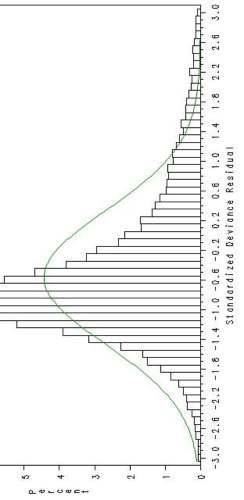
Goodness-of-Fit
• Trying to answer question: How well does our model fit
  the data?
• Can be measured on training data or on holdout data
• By identifying areas of poor model fit, we may be able to
  improve our model
• A few ways to measure goodness-of-fit
  – Squared or absolute error
  – Likelihood/log-likelihood
  – AIC/BIC
  – Deviance/deviance residuals
  – Pearson Chi-Squared
  – Plot of actual versus predicted target

                                                              2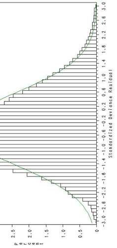
Squared Error & Absolute Error
• For each record, calculate the squared or absolute
  difference between actual and predicted target
  variable

• Easy and intuitive, but generally inappropriate for
  insurance data, and can lead to selection of wrong
  model

• Squared error appropriate for Normal data, but
  insurance data generally not Normal

                                                        3
Likelihood

• The probability, as predicted by our model, that what
  actually did occur would occur

• A GLM calculates the parameters that maximize
  likelihood

• Higher likelihood Æ better model fit (very simple
  terms)

• Problem with likelihood – adding a variable always
  improves likelihood

                                                          4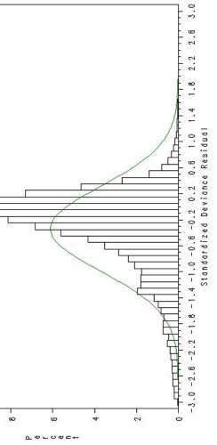
AIC & BIC
• Akaike Information Criterion (AIC) =
   -2*(Log Likelihood) + 2*(Number of Parameters in Model)

• Bayesian Information Criterion (BIC) =
   -2*(Log
    2*(Log Likelihood) + (Number of Parameters in Model)*ln(Number
  of Records in Dataset)

• Penalized measures of fit

• Good rule for deciding which variables to include –
  unless a variables improves AIC or BIC, don’t include it

• BIC often too restrictive

                                                                     5
Deviance
• Saturated model – the model with the highest
possible likelihood
– One indicator variable for each record, so model fits data perfectly
• Deviance = 2*(loglikelihood of saturated model –
loglikelihood of fitted model)
• GLMs minimize deviance
• Like squared error, but reflects shape of assumed
distribution
• We generally fit skewed distributions to insurance
data (Tweedie, gamma, etc), and thus deviance is
more appropriate than squared error
6Deviance – in Math
• Poisson:
• Gamma:
• Tweedie:
• Normal:
7Analysis of Deviance
• Can calculate deviance for each record and
focus on outliers (why is model missing so badly
for those records?)
• Can plot the deviance for each observation to
visually inspect for outliers
• Note that analysis of deviance doesn’t only apply
to GLMs
–As long as we are willing to assume a distribution, we
can calculate deviance
–Deviance can be used for minimum bias procedures
8Plot of Deviance by Record
9Plot of Deviance by Record
10Residuals
• Raw residual = yi – μi, where y is actual value of
target variable and μ is predicted value
• In simple linear regression, residuals are supposed
to be Normally distributed, and departure from
Normality indicates poor fit
• For insurance data, raw residuals are highly skewed
and generally not useful
11Deviance Residuals
• Square root of (weighted) deviance times the sign of
actual minus predicted
• Measures amount by which the model missed, but
reflects the assumed distribution
• Should be approximately Normally distributed, and
far departure from Normality indicates that incorrect
distribution has been chosen
• Ideally, there should be no discernable pattern in
deviance residuals
–Model should miss randomly, not systemically
12Deviance Residual Diagnostics
• Histogram of deviance residuals – look for
approximate Normality (bell-shape)
–Far departure from Normality generally indicates that
incorrect distribution has been chosen
– Can also indicate poor fit
• Scatter plot of deviance residuals versus predicted
target variable
–Should be uninformative cloud
–Pattern in this plot indicates incorrect distribution
13Deviance Residual Diagnostics
• Scatter plot of deviance residuals versus weight
–If weight statement is appropriate, then plot should be
uninformative cloud
• Plot deviance residual for each record and look
for outliers
• Feed deviance residuals into tree algorithm
–If deviance residuals are random, then tree should find no
significant splits
14Example: Selecting Severity Model
• Goal is to select a distribution to model severity
• Two common choices – Gamma and Inverse
Gaussian
–Gamma: V(μ) = μ2
– Variance of severity is proportional to mean severity squared
–Inverse Gaussian: V(μ) = μ3
– Variance of severity is proportional to mean severity cubed
• Two lines of business
–LOB1 is high-frequency, low-severity
–LOB2 is low-frequency, high-severity
15Deviance Residual Histogram
LOB1, Gamma GLM 16Deviance Residual Histogram
LOB1, IG GLM 17Plot of Deviance Residuals versus
Target
LOB1, Gamma GLM 18Plot of Deviance Residuals versus
Target
LOB1, IG GLM 19Deviance Residual Histogram
LOB2, Gamma GLM 20Deviance Residual Histogram
LOB2, IG GLM 21Deviance Residuals Caution
• Analysis of deviance residuals only applicable to
continuous or somewhat-continuous data
• If building a frequency model, and every record
has either 0 or 1 claim, then deviance residuals
will be bimodal
• If can aggregate discrete data to make it
somewhat continuous, then deviance residual
diagnostics may be appropriate
22Actual vs Predicted Target
• Scatter plot of actual target variable (on y-axis)
versus predicted target variable (on x-axis)
• If model fits well, then plot should produce a
straight line, indicating close agreement
between actual and predicted
–Focus on areas where model seems to miss
• If have many records, may need to bucket (such
as into percentiles)
• Depending on scale, may need to plot on a log-
log scale
23Example of Actual vs Predicted
24Example of Log of Actual vs Log of
Predicted
25Benefit of Deviance over Squared
Error
• Since squared error is the deviance of a
regression model with a Normal distribution,
using squared error for non-Normal data can
lead to incorrect model being chosen
• We run two models on our dataset – one with a
Tweedie distribution and one with a Normal
distribution
• Data is far from Normal, but using squared error
as a metric, the Normal GLM wins
–Even absolute error shows the Normal winning
26Log of Actual vs Log of Pred Target
with Normal Linear Regression
27Measuring Internal Stability
• Process of determining how robust our model
results are
• Useful measures:
–Out-of-sample (out-of-time) validation
–Cross-validation
–Plotting actual versus predicted target variable on
holdout data
–Measures of influence (e.g. Cook’s Distance)
–Bootstrapping
28Out-of-Sample Validation
• Important to assess model fit on data that was
not used in model construction
• Two approaches:
– Initially split dataset into training and test, build model on training,
and measure fit on test
– Cross-validate – repeatedly use one subset to build and one to test
• Can randomly split dataset, or can split based on
a control variable (like year)
29Assessing Stability over Time
• Generally want model results to be stable over
time
• To assess temporal stability, can run the model
on individual years and look for variability
–For example, if have 5 years, can run model on just
years 1 and 2, then on just years 2 and 3, etc
–Ideally, the parameter estimates don’t change
significantly across subsets
30Out-of-Sample Deviance
• Use one set to build model and, based on those
results, calculate the deviance of each record in
a holdout dataset
• Look for outlier records (either visually or by
sorting)
31Plot of Actual vs Predicted on
Holdout
• Produce scatter plot of actual target variable
versus predicted target variable as before, but
use one set to build model and another set to
plot
• Very simple diagnostic to produce and
understand, and tells a powerful story
–Easy to explain to non-technical audience
32Example of Plot of Actual vs
Predicted on Holdout
33Cook’s Distance
• Cook’s Distance is an Influence Diagnostic, which
tells us the impact that each record has on model
results
• Larger Cook’s Distance Æ more influence Æ model
results may change significantly if record is removed
• Two uses of Cook’s Distance
–Identifying erroneous records
–Measuring the internal stability of a model
– Delete the 10 records with the largest Cook’s Distance and re-
run the model
– If deleting only a handful of records causes results to change
significantly, then model is not very stable
34Bootstrapping
• Re-sampling technique that allows us to get more
out of our data
• Start with a dataset and sample from it with
replacement
– Some records will get pulled multiple times, and some will not get
pulled at all
• Generally, we create a dataset with the same
number of records as our original dataset
• Can create many bootstrap datasets, and each
dataset can be thought of as an alternate reality
– Since each bootstrap is an alternate reality, we can use
bootstrapping to construct confidence intervals
35Bootstrap CIs for Parameter
Estimates
• GLMs produce confidence intervals for parameter
estimates, but it is valuable to get a second opinion
• Create many bootstrap datasets, re-run
re run the GLM on
each dataset, and construct a confidence interval
based on the resulting parameter estimates
• If bootstrap confidence interval is significantly wider
than that produced by GLM, it is a sign that our
results are overly-influenced by a few records
36Confidence Intervals for Fit
Statistics
• Using bootstrapping, we can put confidence
intervals around deviance or log-likelihood
• If deviance varies widely across the bootstrap
datasets, it is a sign that our results are not very
stable
37Confidence Intervals for Lift
Measures
• Can use bootstrapping to put confidence intervals
around lift measures, like Gini indices
• In measuring lift, we seek to answer the question: Does
Model A outperform Model B?
• If the answer is yes, then the second question is: How
significant is the win?
• Say Model A has a Gini index of 15.90 and Model B has
a Gini index of 15.40
– Model A has a Gini index that is 0.50 higher, but is that difference
significant?
• Can also bootstrap quantile plots and double lift charts
38References
• Anderson, Duncan, et. al., A Practitioner’s Guide to
Generalized Linear Models, CAS Discussion Paper Program,
2004, pp. 1-116.
• De Jong, Piet and Heller, Gillian, Generalized Linear Models
for Insurance Data, Cambridge University Press, 2008
• Efron, Bradley and Tibshirani, Robert, An Introduction to the
Bootstrap, Chapman & Hall, 1994
• McCullagh, P. and J. A. Nelder, Generalized Linear Models,
2nd Ed., Chapman & Hall, 1989
• Werner, Geoff and Claudine Modlin, Basic Ratemaking,
Casualty Actuarial Society, Fourth Edition, October 2010.
39And The Winner Is…?
How to Pick a Better Model
Part 2 – Goodness-of-Fit and Internal Stability
Dan Tevet, FCAS, MAAA
40You can also read